自願捐獻與租稅順從之實驗研究

行政院國家科學委員會專題研究計畫 成果報告

自願捐獻與租稅順從之實驗研究

計畫類別： 個別型計畫 計畫編號： NSC93-2415-H-004-008- 執行期間： 93 年 08 月 01 日至 95 年 01 月 31 日 執行單位： 國立政治大學財政系 計畫主持人： 徐麗振 共同主持人： 宋玉生 計畫參與人員： 張家瑋，賴冠宇 報告類型： 精簡報告 處理方式： 本計畫可公開查詢

中 華 民 國 95 年 4 月 27 日

Tax Audit and Voluntary Public Good Provision:

Experimental Evidence

Li-Chen Hsu*

Abstract: We conduct seven experiments to explore how the incentives of voluntary

contributions and income reporting are affected by changes in marginal per capita returns of publicly and privately provided public and some tax parameters, for instance, marginal tax rates and audit probabilities. We find that if subjects’ tax payments vary with their reported income, the increase in either the marginal per capita return of privately provided public good or the marginal per capita return of publicly provided public good will induce significantly more voluntary contributions. However, the former change has no effect on income reporting, but the latter can greatly improve honest reporting. Furthermore, the change in the marginal tax rate has no effect on both voluntary contributions and income reporting. The increase in audit probability has no effect on voluntary contributions, either, but can alleviate cheating. Given the evidence above, we conclude that enhancing the efficiency in providing the publicly provided public good is the most effective way to induce more voluntary contributions and honest reporting.

Keywords: Experiments, Public Goods, Tax Audit JEL Classification: C92, H26, H41

*

Department of Public Finance, National Chengchi University, 64, Sec. 2, Chih-Nan Rd., Taipei 11605, Taiwan; Tel: (886) 2-2938-7313; Fax: (886) 2-2939-0074; e-mail: lchsu@nccu.edu.tw. Financial support from the National Science Council (grant number: NSC 93-2415-H-004-008) is gratefully acknowledged. 本計畫原共同主持人台 大經濟系宋玉生副教授，於本計畫開始進行之初，即表明因其家庭因素，無暇參與本計畫，故本計畫自構思 至實驗操作，乃至最後的結果分析與報告撰寫，宋副教授皆未曾參與。

摘要： 在本研究中我們操作七個實驗，探討自願捐獻與所得申報的動機如何受到私人與政 府提供公共財的邊際每人報酬，以及某些租稅變數（例如邊際稅率與稽核率）影響。我們 發現當實驗參與者的稅負因他們所申報所得的不同而不同時，私人與政府提供公共財的邊 際每人報酬的增加都可明顯提高自願捐獻。然而，前者的改變不影響所得申報，但後者卻 能顯著改善誠實申報。此外，邊際稅率的改變不影響自願捐獻與所得申報。稽核率的提高 也不影響自願捐獻，但卻能減漏報動機。基於上述實驗證據，我們推斷加強公部門提供公 共財的效率為提高自願捐獻與誠實申報的最有效良方。 關鍵詞：實驗，公共財，租稅稽核 JEL 分類: C92, H41

1. INTRODUCTION

The literature of tax evasion has developed to be a very vivacious field since Allingham and Sandom’s (1972) pioneering theoretical paper. In Allingham and Sandom’s model the tax payer is endowed with an exogenous income y. He reports income x (x≤ ) to the tax authority and y pay taxes tx, where t is his marginal tax rate. The tax authority has no information regarding the tax payer’s real income, but it can audit it with probability p. The probability p is exogenously given. If the tax payer was caught cheating, besides paying the evaded taxes, he had to pay a fine of θ on each dollar he evaded. The tax payer’s problem is to maximize his expected utility by choosing x.

Allingham and Sandom found that increasing p and θ can induce the tax payer to report a higher income, but the effect of changes in t is ambiguous. The reason is that under the assumption of decreasing absolute risk aversion, the increase in t reduces the tax payer’s after-tax income. The tax payer becomes more risk averse and therefore reduces cheating. However, the increase in t also raises the marginal return from tax evasion. So the tax payer will evade more income due to the substitution effect. As a consequence, the effect of changes in t on income evading is ambiguous. In a later work, Yitzhaki (1974) assumes that the fine is imposed on the evaded tax rather than on the evaded income and finds that the increase in the marginal tax will surely reduce cheating. The reason is that though the marginal return from tax evasion is higher when the marginal tax rate is higher, in the meantime the fine is also higher. Both the income and substitution effects work in the same direction and as a result tax evasion is alleviated when t increases.

The effects of changes in tax parameters on tax evasion have been examined by many subsequent experimental studies. Most of these studies follow Allingham and Sandom’s (1972)

theoretical model, but modify it in several ways. For instance, experimental studies generally assume that tax payers maximize expected income rather than expected utility. In other words, tax payers are assumed to be risk neutral. Yitzhaki’s (1974) assumption that the fine is imposed on the evaded taxes is also used. Furthermore, some experimental studies examine the effect of audit probability when it is not exogenously given but varies with income.

Spicer and Thoman (1982), Spicer and Hero (1985), and Alm, Jackson, and McKee (1992a) investigate how the tax system uncertainty affects tax compliance. Spicer and Thomas (1982) specifically explore whether the reported income is affected by audit procedures. Fifty-four subjects are divided evenly in three groups. One group is informed that the audit probability is either 5 percent, 15 percent, or 25 percent, another group is only informed that audit probability may be high, medium, or low, and the rest group has none of information regarding audit probability. Spicer and Thomas (1982) find that tax evasion is significantly lower in the group that is specifically informed about the audit probability.

Spicer and Hero (1985) examine whether the reported income is affected by other taxpayers’ cheating behavior. They recruit 36 subjects, in which 12 subjects are informed that participants in the previous experiment (actually it is non-existed) paid only 10 percent of required taxes, another 12 subjects are informed that this number is 50 percent, and the rest 12 subjects are informed that this number is 90 percent. They find that tax evasion is not affected by the amount of other tax payers’ evaded taxes.

Alm, Jackson, and McKee (1992a), on the other hand, investigate respectively whether tax evasion is affected by the uncertainty in fine, tax rates, and audit probabilities. They find that if tax revenues are not used to fund public goods, then the uncertainty in the above variables can always induce tax compliance. On the contrary, if tax revenues are used to provide public

goods, then uncertainty will instead lower tax compliance. Furthermore, their evidence shows that tax compliance is higher in the experiment with public goods than in the experiment without public goods despite whether the uncertainty exists or not.

Similar to Alm, Jackson, and McKee (1992a), Becker, Büchner, and Sleeking (1987), Alm, Jackson, and McKee (1992b), and Alm, McClelland, and Schulze (1992) also consider public expenditures. Specifically, Becker, Büchner, and Sleeking (1987) examine the effect of transfer payments. They find that if subjects perceive that their transfer payments are lower than what other subjects receive, then higher levels of tax evasion will result. Alm, Jackson, and McKee (1992b) put tax-funded public goods into subjects’ payoff function, but differing from their previous paper, no uncertainty exists in any tax variables. Thy find that increases in audit probabilities and fine can improve tax compliance, but the effects are minor. In addition, tax compliance is also higher when the tax rate is lower and taxes are used to fund public goods. Finally, Alm, McClelland, and Schulze (1992) consider different magnitudes of group surplus multiplier. They find that the higher audit probabilities and higher group surplus multipliers significantly raise tax compliance.

We can observe from the review above that some experimental studies ignore the use side of tax revenues. For those studies that do deal with tax revenues, they consider only tax-funded public goods, despite the fact that privately provided public goods are prevalent in the real world. Therefore, in this paper we consider two types of public goods: publicly and privately provided public goods. We vary the marginal per capita returns of the two public goods and the magnitudes of tax rates and audit probabilities in various experiments. We intend to observe how the incentives of voluntary contributions and honest reporting are affected by these variables. The next section provides a simple model of tax evasion and the experimental design. In

Section 3 we present experimental results. Section 4 concludes.

2. EXPERIMENTAL DESIGN

2.1. The Model

Consider an economy of n individuals. Individual i is endowed with an exogenous income

i

y . He reports income x , _i x_i ≤ , to the tax authority and pays the taxes according to his y_i reported income. It is assumed that his average tax rate (which is equal to his marginal tax rate) is t, t<1, so that individual i’s tax payment is tx . After reporting, the tax authority audits tax i

payers’ real incomes by a probability p. If caught cheating, then besides paying the evaded tax )

(yi xi

t − , there is a fine. It is assumed that the fine is θ times the evaded tax so that the fine is θt(yi −xi). After paying taxes and the fine, if there is any, individual i allocates the rest of his income between a voluntary contribution c to a privately provided public good Z and his _i

private good consumption. The size of Z is therefore =

∑

n₌

j cj

Z

1 . In addition, it is assumed

that all the government budget is balanced such that all taxes and fines are used to funded a publicly provided public good Y. That is, =

∑

₌ +

∑

_j∈A j− j +

∑

_j∈A j − j

n

j txj t y x t y x

Y ₁ ( ) θ ( ),

where A is the set of tax payers who are caught cheating.

The marginal per capita return of Y is m. That is, each dollar of taxes or fines paid by anyone yields each person a return of m. So the marginal social return of Y is nm. On the other hand, the marginal per capita return of Z is r. In other words, each individual gains a return of r for every dollar donated by anyone. As a result, the marginal social return of Z is nr. Notice that m and r need to meet the condition 1/n<m,r<1. This is because if m and r are

greater than one, then everyone would donate all of his income or pay taxes as large as he could. By contrast, if m and r are less than 1/n, then no one wants to donate and will try his best to escape the tax.

Like many other experimental studies on tax evasion, here we assume individual i’s utility function is linear and i pursues the maximum expected return EP_i. Therefore, we can write individual i’s problem as:

} ] ) ( ) ( [ ) ( ){ 1 ( } ] ) ( ) ( ) ( ) ( [ ) ( ) ( ) ( { ,

∑

∑

∑

∑

∑

∑

∑

∑

≠ ∈ ≠ ∈ ≠ ≠ ≠ ∈ ≠ ∈ ≠ ≠ − + − + + + + + − − − + − + − + + − + − + + − − − − + + − − = i j A j i j A j _{j j} j j i j j i i j j i i i i i j A j i j A j _{j j} j j i j j i i i i i i i i i i j j i i i i i i i x y t x y t tx tx m c c r tx c y p x y t x y t tx x y t x y t tx m x y t x y t c c r tx c y p EP c x Max θ θ θ θ

The first-order conditions are:

) 1 )( 1 ( m p p t x EP i i = − − + ∂ ∂ _θ (1) 0 1+ < − = ∂ ∂ r c EP i i . (2)

Equation (1) implies that if (pθ + p)<1, then xi =0; if (pθ + p)>1, then xi = ; and yi

only if (pθ +p) is exactly equal to 1, we have an interior solution x_i< . Since both p and y_i θ are constants, the chance for equation (1) to be equal to zero is slim. For instance, if p = 0.05, then the fine must be 19 times the evaded tax for equation (1) to bind.

Equation (2) says that the individual’s donation to the privately provided public good (Z) is zero. This is straightforward since under the linear payoff function everyone has an incentive not to donate as long as r < 1. Notice from equation (2) that the magnitudes of t, θ , and p will

not affect the individual’s donating decisions.

2.2. Experimental Parameters

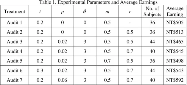
Table 1 summarizes the seven experiments that we conducted. By comparing these experiments, we can test the effects of changes in tax rates, audit probabilities, fines, and the marginal per capita returns on the public goods provided by the public and private sectors on the reported income and contributions. Thirty-six to forty-four subjects were used in each experiment, depending on how many subjects eventually showed up. Subjects were recruited from intermediate economics classes at National Chengchi University. None of them had ever participated in any public goods experiments. In each experiment subjects were randomly and anonymously assigned to groups of four and they stayed in the same groups for all 12 rounds. In each round the four group members were randomly assigned the income NT$15, NT$20, NT$25, and NT$30, respectively. They were informed that when the new round started, each of them would be reassigned a new level of income. They knew their own income and the distribution of income, but not the other three group members’ levels of income.

The experiments of Audit 1 and Audit 2 serve as the benchmark experiments. In Audit 1, a lump-sum tax of tax rate 0.2 is imposed on each subject’s income. Subjects only decide the amount of money contributing to the public good and they need not to report their income. Therefore, they have no incentive to evade the tax. All taxes collected and voluntary contributions are used to fund the public good Y. Audit 2 is the same as Audit 1 in every respect except that the public good Y is only funded by taxes and voluntary contributions go to another public good Z. By comparing the difference between the two experiments we can observe that whether individual contributions differ when both publicly and privately provided

public goods co-exist.

We incorporated an audit mechanism into Audit 3 through Audit 7. We put 50 balls in a transparent bag, with the numbers 1 through 50 written on each ball. When conducting Audit 3, we draw one ball from the bag so that the audit probability is 0.02. The subject with the subject number same as that on the ball drawn is audited and he will pay a fine which is three times the evaded tax if he is caught cheating. The tax rate and the marginal per capita returns of both public goods remain the same as those in Audit 2. In Audit 4, we raise the marginal per capita return of the public good Z to 0.7. By comparing Audit 4 with Audit 3, we can observe whether a relatively more efficient privately provided public good induces more voluntary contributions and cheating. Alternatively, we raise the marginal per capita return of the public good Y to 0.7 in Audit 5. As a consequence, comparing Audit 5 with Audit 3 tells us whether a relatively more efficient publicly provided public good discourages (crowd-out) voluntary contributions and encourages honest reporting. Both Audit 6 and Audit 7 are the same as Audit 4 in every respect except that the tax rate in Audit 6 is raised to 0.3 and the audit probability in Audit 7 increases to 0.06. By comparing Audit 6 with Audit 4, we can see the effect of tax rate increasing, and by comparing Audit 7 with Audit 4, the effect of the increase in audit probability.

3. RESULTS

Our experimental design, like many others in public goods experiments, are repeated, thus allow subjects to learn about both the game and the reactions from their opponents. As was mentioned by Andreoni and Miller (2002), this suggests looking at the first round, since subjects have not gained any experience. However, Andreoni and Miller also pointed out that forward-looking subjects may play strategically, and thereby looking at the final round may be

more suitable since by then strategic plays are unnecessary. Fehr and Schmidt (1999, Quarterly Journal of Economics, p. 843) also suggest looking at the final round. They noted that “… we take the data of the final period as the facts to be explained. There are two reasons for this choice. First, it is well-known in experimental economics that in interactive situations one cannot expect the subjects to play an equilibrium in the first period already. … Second, if there is repeated interaction between the same opponents, then there may be repeated games effects that come into play. These effects can be excluded if we look at the last period only.” Given these opinions, we shall particularly look at the final round, but we shall also give brief descriptive statistics of the first round and the whole repetitions.

We shall begin by looking at the detailed data from each experiment and ask how well our data conform to the theoretical predictions. Then we shall explore more closely the differences between experiments and between different levels of income.

3.1. Comparing the Data with the Theoretical Predictions

Figures 1-a through 1-c depict the ratios of contributions to income per round in various treatments. It can be easily seen subjects started contributing an average of 34 to 47 percent of their income to the public good. Contributions decay over rounds in all treatments and in the final round the average contributions are about 13 to 28 percent of subjects’ income. Sum over all rounds, subjects in Audit 7 contributed the most, which is about 41 percent of their income. By contrast, Audit 5 has the least average contributions, in which subjects contributed an average of 25 percent of their income. All of these numbers are much higher than zero, contradicting the theoretical prediction that subjects should contribute nothing to the public good.

if (pθ + p)>1, then xi = ; and only if yi (pθ+p) is exactly equal to 1, we have an interior

solution x_i < . Given the audit probabilities (p = 0.02 or 0.06) and the fine rate (y_i θ =3) used in the experiments, it is obvious that (pθ + p)<1. Therefore, we should observe that the reported income is zero. Again, the experimental evidence differs sharply from this theoretical prediction.

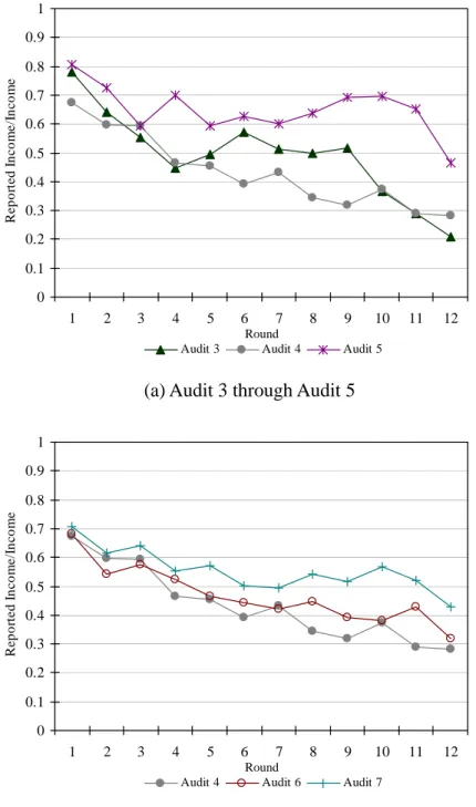
Figures 2-a and 2-b depict the average ratios of reported income to income per round in treatments Audit 3 through Audit 7. It can be seen that subjects in all treatments started reporting 68 to 80 percent of their income on average. The reported income decays over rounds and in the final round reported income accounts for 21 to 46 percent of subjects’ real income. Sum over all 12 rounds, Audit 5 has the highest ratio of reported income to income (65 percent) and Audit 4 has the least (44 percent). These magnitudes differ from the theoretical prediction that subjects should report zero given the audit probabilities and fine rate.

3.2. Comparing the Data across Various Treatments A. Voluntary Contributions

We first compare the results from the two benchmark experiments, i.e., Audit 1 and Audit 2. It can be seen from Figure 1-a that except in round three subjects in Audit 2 contributed a higher fraction of their income to the public good than did subjects in Audit 1. However, the difference seems subtle before round ten. A two-sided Mann-Whitney U test shows that the difference between these two treatments is statistically insignificant, regardless of looking at the first round, the final round, the average of round 1 through round 4, round 5 through round 8, round 9 through 12, or the entire 12 rounds. Table 2 reports these statistical results. A two-sided Kolmogorov-Smirnov test shows similar statistics, which are reported in Table 3.

This evidence says that when the marginal per capita returns of publicly and privately provided public goods are the same, subjects are indifferent to which public good to give. Given this result, we use two separate public goods in the remaining treatments with tax auditing.

Let us now start comparing the results from Audit 3 and Audit 2. Looking at Figure 1-a again, we can observe that subjects in these two treatments give about the same fraction of income to the privately provided public good in the first round. The difference enlarges after that, but then disappears starting round six, and appears again as the final round arrives. A two-sided Mann-Whitney U test shows that subjects in Audit 3 give a smaller fraction of income to the privately provided public good than do subjects in Audit 2 in round 1 through round 4 and in the final round. A Kolmogorov-Smirnov test confirms the results from round 1 through round 4, though the difference in the final round is insignificant. We have the following observation.

Observation 1: If subjects’ tax payments vary with their reported income and they are constrained to face an audit probability and penalty, then they will make fewer voluntary contributions as compared with the case if they pay a fixed amount of taxes.

Observation 1 suggests that when subjects can reduce the enforced contributions (taxes) by cheating, though they may not choose to do so, they will reduce the voluntary contributions as well.

We now ask how the change in the marginal per capita return of the privately provided public good affects voluntary contributions. This can be done by comparing Audit 3 with Audit 4. As shown by Figure 1-b, subjects in Audit start to give an average 36 percent of their

income to the privately provided public good, which is about the same as that in Audit 3. These fractions are higher in Audit 4 than in Audit 3 in all of the following rounds, and in the final round it is 25 percent in Audit 4 and 13 percent in Audit 2. A two-sided Mann-Whitney U test shows that in the final round the difference between these two treatments is significant, and it is marginally significant by using a Kolmogorov-Smirnov test. We have Observation 2 below:

Observation 2: If subjects’ tax payments vary with their reported income and if the marginal per capita return of the tax-funded public goods remains the same, then the increase in the marginal per capita return of voluntarily provided public good will induce significantly more voluntary contributions.

We now ask alternatively how the change in the marginal per capita return of the publicly provided public good affects voluntary contributions. This can be seen by comparing Audit 3 with Audit 5. As shown by Figure 1-b, subjects in both treatments start to give about the same fraction of income to the privately provided public good in round one. This situation maintains until round 3. In middle rounds of the game subjects in Audit 3 give a higher fraction of income than do subjects in Audit 5, but then the opposite is observed in latter rounds. As is reported in Table 2, a two-sided Mann-Whitney U test shows that this fraction is marginally higher in Audit 3 than in Audit 5 in rounds 5 through 8, but the difference is only marginally significant. The opposite is observed in the final round the difference is significant. We therefore have Observation 3 below:

capita return of the privately provided public goods remains the same, then the increase in the marginal per capita return of the tax-funded public good will induce significantly more voluntary contributions.

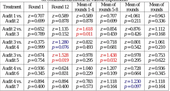
We now use Audit 4 as the base treatment and investigate how the change in tax rate (Audit 6) and audit probability (Audit 7) affects voluntary contributions. As shown by Figure 1-c, Audit 7 has the highest fraction of contributions to income in every round of the game. However, a Mann-Whitney U test shows that subjects in Audit 7 contribute a larger fraction of income than do subjects in Audit 4 only when we look at round one, the average of rounds 9 through 12, and the average of rounds 1 through 12, and the differences are only marginally significant. Comparing Audit 4 with Audit 6, we find that except in round one and the final three rounds, the fraction of contributions to income in each of the rest rounds is higher in Audit 4 than in Audit 6. However, a Mann-Whitney U test shows that the difference is insignificant, regardless of looking at which periods of the game. We summarize these results in Observation 4 below:

Observation 4: The changes in the marginal tax rate and audit probability have no significant effect on voluntary contributions.1

B. Reported Income

Figure 2-a and 2-b draw the average ratios of reported income to subjects’ income per round

1

These results may be different if we used m = 0.5 and r = 0.5 in Audit 6 and Audit 7 and compared the resulted data with those in Audit 3. In other words, results in Observation 4 can only say that when r is higher than m, the increase in tax rate and audit probability does not affect voluntary contributions. However, if r equals m, then results may differ. This comparison may be worthy to explore, but we did not conduct such experiments due to the

in treatments Audit 3 through Audit 7. Let us begin by exploring how the changes in the marginal per capita returns of publicly and privately provided public goods affect subjects’ incentive of honest reporting. Figure 2-a shows that in the middles rounds (round 5 through round 9) of the game the average ratios of reported income to income are higher in Audit 3 than in Audit 4, but the two are almost coincide in early rounds and final rounds. A two-sided Mann-Whitney U test confirms that subjects in Audit 3 report a larger fraction of income than do subjects in Audit 3 when we look at round one and the average of round 5 through round 8, and the differences are only marginally significant. A two-sided Kolmogorov-Smirnov test, on the other hand, shows no significant difference, regardless of looking at which periods of the game. We report these statistics in Table 4 and Table 5 and summarize the results in Observation 5 below.

Observation 5: The increase in the marginal per capita return of the privately provided public good has no effect on income reporting.

Let us now compare Audit 3 with Audit 5. Figure 2-a shows that subjects in these two treatments report similar fractions of income (78 percent in Audit 3 and 80 percent in Audit 5). These fractions decrease over rounds in both treatments, and the differences between them increase over rounds, especially after round 6. In the final round of the game, subjects in Audit 3 and Audit 5 report 21 percent and 46 percent of their income, respectively. Both two-sided Mann-Whitney U and Kolmogorov-Smirnov tests show that subjects in Audit 5 report significantly a larger fraction of income than do subjects in Audit 3 when we look at the final round, the average of round 9 through round 12, and the average of entire 12 rounds. Here

comes Observation 6:

Observation 6: The increase in the marginal per capita return of the publicly provided public good greatly improves honest reporting.

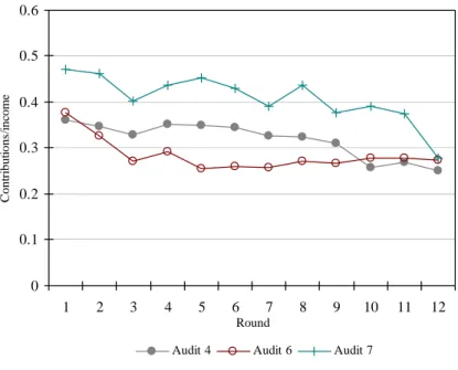
Finally let us explore how the changes in tax rate and audit probability affect honest reporting. It can be seen from Figure 2-b that the fractions of reported income to income are similar in every round of Audit 4 and Audit 6, though overall the average fraction is higher in Audit 6 (47 percent) than in Audit 4 (44 percent). Both two-sided Mann-Whitney U and Kolmogorov-Smirnov tests show no significant difference, regardless of looking at which periods of the game.

On the contrary, it can be easily seen from Figure 2-b that the difference between Audit 4 and Audit 7 is more salient, especially in latter rounds of the game. Subjects in the two treatments report similar fractions of income (67 percent in Audit 4 and 71 percent in Audit 7). The difference between these two grows over rounds, with an average of 44 percent in Audit 4 and 55 percent in Audit 7. A two-sided Mann-Whitney U test shows that the difference is significant by looking at the average of round 9 through round 12, and is marginally significant if we look at the final round and the average of round 5 through 8. A two-sided Kolmogorov-Smirnov test shows similar results. These statistics are reported in Table 4 and Table 5. We now have our last observation below:

increase in audit probability can alleviate cheating.2

4. SUMMARY AND CONCLUSION

We conduct seven experiments and try to explore whether the change in the marginal per capita returns of both publicly and privately provided public goods affect subjects’ incentives to give and to report income honestly. We also examine whether these incentives are affected by some tax parameters, for instance, tax rates and audit probabilities. Our major findings are the following: First, if subjects’ tax payments vary with their reported income and if they are subject to tax auditing, they will make fewer voluntary contributions as compared with the case if they pay a fixed amount of taxes. Second, if subjects’ tax payments vary with their reported income, the increase in either the marginal per capita return of privately provided public good or the marginal per capita return of the publicly provided public good will induce significantly more voluntary contributions. Third, the increase in the marginal per capita return of the privately provided public good has no effect on income reporting, but the increase in the marginal per capita return of the publicly provided public good greatly improves honest reporting. Fourth, the change in the marginal tax rate has no significant effect on both voluntary contributions and income reporting. Fifth and finally, the increase in audit probability has no significant effect on voluntary contributions, but can alleviate cheating. Given these results, we can see that enhancing the efficiency in providing the publicly provided public good is the most effective way to induce more private contributions and honest reporting.

2

Table 1. Experimental Parameters and Average Earnings Treatment t p θ m r No. of Subjects Average Earning Audit 1 0.2 0 0 0.5 - 36 NT$505 Audit 2 0.2 0 0 0.5 0.5 36 NT$513 Audit 3 0.2 0.02 3 0.5 0.5 44 NT$465 Audit 4 0.2 0.02 3 0.5 0.7 40 NT$545 Audit 5 0.2 0.02 3 0.7 0.5 36 NT$498 Audit 6 0.3 0.02 3 0.5 0.7 44 NT$543 Audit 7 0.2 0.06 3 0.5 0.7 40 NT$592

Note: The variable t denotes the tax rate, p the audit probability, θ the fine rate, m the marginal per capita return of the public good funded by taxes (Y), and r the marginal per capita return of the public good funded by donations (Z).

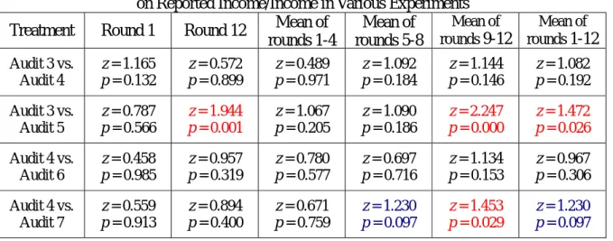
Table 2. The Results of Two-Sided Mann-Whitney U Tests on Contributions/Income in Various Experiments Treatment Round 1 Round 12 Mean of

rounds 1-4 Mean of rounds 5-8 Mean of rounds 9-12 Mean of rounds 1-12 Audit 1 vs. Audit 2 z =－0.792 p = 0.428 z =－0.083 p = 0.934 z =－0.547 p = 0.585 z =－0.586 p = 0.558 z =－0.767 p = 0.443 z =－1.087 p = 0.277 Audit 2 vs. Audit 3 z = 0.485 p = 0.627 z = 1.993 p = 0.046 z = 2.124 p = 0.034 z = 1.070 p = 0.285 z = 1.247 p = 0.212 z = 1.804 p = 0.071 Audit 3 vs. Audit 4 z =－0.077 p = 0.939 z =－2.367 p = 0.018 z =－0.995 p = 0.320 z =－0.923 p = 0.356 z =－0.993 p = 0.321 z =－1.156 p = 0.248 Audit 3 vs. Audit 5 z =－0.422 p = 0.673 z =－2.557 p = 0.011 z =－0.498 p = 0.618 z = 1.650 p = 0.099 z =－0.974 p = 0.330 z = 0.048 p = 0.961 Audit 4 vs. Audit 6 z =－0.337 p = 0.736 z =－0.798 p = 0.425 z = 0.887 p = 0.375 z = 1.421 p = 0.155 z =－0.229 p = 0.819 z = 0.932 p = 0.351 Audit 4 vs. Audit 7 z =－1.750 p = 0.080 z =－1.058 p = 0.290 z =－1.632 p = 0.103 z =－1.463 p = 0.143 z =－1.845 p = 0.065 z =－1.708 p = 0.088

Table 3. The Results of Two-Sided Kolmogorov-Smirnov Tests on Contributions/Income in Various Experiments

Treatment Round 1 Round 12 Mean of rounds 1-4 Mean of rounds 5-8 Mean of rounds Mean of rounds Audit 1 vs. Audit 2 z = 0.707 p = 0.699 z = 0.589 p = 0.878 z = 0.589 p = 0.878 z = 0.707 p = 0.699 z =1.061 p = 0.211 z = 0.943 p = 0.336 Audit 2 vs. Audit 3 z = 0.652 p = 0.789 z = 1.135 p = 0.152 z = 1.618 p = 0.011 z = 0.854 p = 0.459 z =0.876 p = 0.426 z = 1.112 p = 0.168 Audit 3 vs. Audit 4 z = 0.375 p = 0.999 z = 1.280 p = 0.076 z = 0.832 p = 0.493 z = 0.718 p = 0.681 z = 0.801 p = 0.542 z = 1.061 p = 0.210 Audit 3 vs. Audit 5 z = 0.674 p = 0.754 z = 1.528 p = 0.019 z = 0.978 p = 0.295 z = 1.438 p = 0.032 z = 0.978 p = 0.295 z = 0.753 p = 0.622 Audit 4 vs. Audit 6 z = 0.936 p = 0.345 z = 0.624 p = 0.831 z = 1.040 p = 0.229 z = 1.207 p = 0.109 z = 0.728 p = 0.664 z = 0.936 p = 0.345 Audit 4 vs. Audit 7 z = 0.894 p = 0.400 z = 0.894 p = 0.400 z = 0.783 p = 0.573 z = 1.118 p = 0.164 z = 1.230 p = 0.097 z = 1.118 p = 0.164

Table 4. The Results of Two-Sided Mann-Whitney U Tests on Reported Income/Income in Various Experiments Treatment Round 1 Round 12 Mean of

rounds 1-4 Mean of rounds 5-8 Mean of rounds Mean of rounds Audit 3 vs. Audit 4 z = 1.862 p = 0.063 z =－0.863 p = 0.388 z = 0.166 p = 0.868 z = 1.709 p = 0.087 z = 0.935 p = 0.350 z = 0.909 p = 0.363 Audit 3 vs. Audit 5 z = 0.440 p = 0.660 z =－3.416 p = 0.001 z =－1.437 p = 0.151 z =－1.553 p = 0.120 z =－4.120 p = 0.000 z =－3.062 p = 0.002 Audit 4 vs. Audit 6 z = 0.275 p = 0.783 z =－1.101 p = 0.271 z = 0.475 p = 0.635 z =－0.744 p = 0.457 z =－1.359 p = 0.174 z =－0.654 p = 0.513 Audit 4 vs. Audit 7 z =－0.730 p = 0.466 z =－1.673 p = 0.094 z =－0.534 p = 0.593 z =－1.734 p = 0.083 z =－2.512 p = 0.012 z =－1.925 p = 0.054

Table 5. The Results of Two-Sided Kolmogorov-Smirnov Tests on Reported Income/Income in Various Experiments Treatment Round 1 Round 12 Mean of

rounds 1-4 Mean of rounds 5-8 Mean of rounds 9-12 Mean of rounds 1-12 Audit 3 vs. Audit 4 z = 1.165 p = 0.132 z = 0.572 p = 0.899 z = 0.489 p = 0.971 z = 1.092 p = 0.184 z = 1.144 p = 0.146 z = 1.082 p = 0.192 Audit 3 vs. Audit 5 z = 0.787 p = 0.566 z = 1.944 p = 0.001 z = 1.067 p = 0.205 z = 1.090 p = 0.186 z = 2.247 p = 0.000 z = 1.472 p = 0.026 Audit 4 vs. Audit 6 z = 0.458 p = 0.985 z = 0.957 p = 0.319 z = 0.780 p = 0.577 z = 0.697 p = 0.716 z = 1.134 p = 0.153 z = 0.967 p = 0.306 Audit 4 vs. Audit 7 z = 0.559 p = 0.913 z = 0.894 p = 0.400 z = 0.671 p = 0.759 z = 1.230 p = 0.097 z = 1.453 p = 0.029 z = 1.230 p = 0.097

0 0.1 0.2 0.3 0.4 0.5 0.6 1 2 3 4 5 6 7 8 9 10 11 12 Round C o n tr ib u tio n s/in co me

Audit 1 Audit 2 Audit 3

(a) Audit 1 through Audit 3

0 0.1 0.2 0.3 0.4 0.5 0.6 1 2 3 4 5 6 7 8 9 10 11 12 Round C o n tr ib u tio n s/in co m e

Audit 3 Audit 4 Audit 5

0 0.1 0.2 0.3 0.4 0.5 0.6 1 2 3 4 5 6 7 8 9 10 11 12 Round C o n tr ib u tio n s/in co me

Audit 4 Audit 6 Audit 7

(c) Audit 4, Audit 6, and Audit 7

0 0.1 0.2 0.3 0.4 0.5 0.6 0.7 0.8 0.9 1 1 2 3 4 5 6 7 8 9 10 11 12 Round R e por te d I n c o m e /I nc o m e

Audit 3 Audit 4 Audit 5

(a) Audit 3 through Audit 5

0 0.1 0.2 0.3 0.4 0.5 0.6 0.7 0.8 0.9 1 1 2 3 4 5 6 7 8 9 10 11 12 Round R e por te d I n c o m e /I nc o m e

Audit 4 Audit 6 Audit 7

(b) Audit 4, Audit 6, and Audit 7

Figure 2. The Average Ratios of Reported Incomes to Incomes by Round

REFERENCES

Allingham, M.G. and A. Sandmo (1972), “Income Tax Evasion: A Theoretical Analysis,”

Journal of Public Economics, 1, 323-338.

Alm, J., B.R. Jackson, and M. McKee (1992a), “Institutional Uncertainty and Taxpayer Compliance,” American Economic Review, 82, 1018-1026.

Alm, J., B.R. Jackson, and M. McKee (1992b), “Estimating the Determinants of Taxpayer Compliance with Experimental Data, National Tax Journal, 45, 107-114.

Alm, J., G.H. McClelland, and W.D. Schulze (1992), “Why Do People Pay Taxes?” Journal

of Public Economics, 48, 21-38.

Andreoni, J. and J. Miller (2002), “Giving According to GARP: An Experimental Test of the Consistency of Preferences for Altruism,” Econometrica, 70, 737-753.

Becker, W., H. Büchner, and S. Sleeking (1987), “The Impact of Public Transfer Expenditures on Tax Evasion: An Experimental Approach,” Journal of Public

Economics, 34, 243-252.

Fehr, E. and K.M. Schmidt (1999), “A Theory of Fairness, Competition, and Cooperation,” Quarterly Journal of Economics, 114, 817-868.

Spicer, M.W. and R.E. Hero (1985), “Tax Evasion and Heuristics,” Journal of Public

Economics, 26, 263-267.

Spicer, M.W. and J.E. Thomas (1982), “Audit Probabilities and the Tax Evasion Decision: An Experimental Approach,” Journal of Economic Psychology, 2, 241-245.

Yitzhaki, S. (1974), “A Note on Income Tax Evasion: A Theoretical Analysis,” Journal of