Time-Optimal Control for a Robotic Contour Following Problem

(1)

Time-Optimal Control for a Robotic Contour

Following Problem

Abstract-A robotic contour following problem, defined by a unilater- ally constrained manipulator, is presented. Our approach explicitly takes into account inequality constraints and resulting contact forces as part of the system dynamics. Possible impact at an entry time is also discussed. A

phase plane technique is applied to the time-optimal motion planning problem subject to conditions of impact avoidance. The contact force is

incorporated into the optimal planning problem. Finally, an example robotic contour following task performed by a planar Cartesian robot is

used to illustrate the ideas developed in the paper.

I. INTRODUCTION

NUMBER of robot or manipulator tasks can be

A

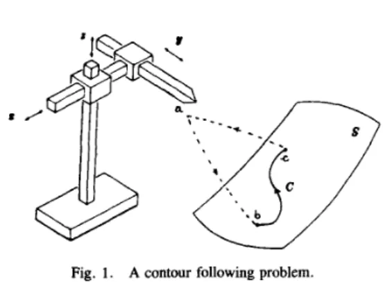
characterized as contour following tasks, including scribing, writing, and possibly debumng and grinding. A specific contour following problem can be stated as follows: assume the end effector of the manipulator is not initially in

contact with a constraint surface S (see Fig. l), then

1) move the end effector from its initial position a to point

b

in surface S;

2) move the end effector along a specified curve C in

S

from point b to point c so that it has a given specified contact force with S;

3) move the end effector from point c back to its initial position a.

The motion of the manipulator consists of two parts: an unconstrained motion, where the end effector is not in contact with the constraint surface

S

(i.e., from point a to point b and from point c to point a in Fig. l), and a constrained motion, where the end effector is in contact with the constraint surface

S (i.e., from point b to point c in Fig. 1). During the unconstrained motion, we have an open kinematic chain

configuration. On the other hand, during the constrained motion, where the contact force must be considered, we have a

closed kinematic chain configuration. For these types of Manuscript received August 27, 1986; revised March 19, 1987. This work was partially supported by the Air Force Office of Scientific Research under AFOSR Contract F 49620-82-COO89 and the Center for Research on Integrated Manufacturing (CRIM) at the University of Michigan. Any opinions, findings, and conclusions or recommendations expressed in this publication are those of the authors and do not necessarily reflect the viewpoint of the sponsors. Part of the material in this paper was presented at the IEEE International Conference on Robotics and Automation, Raleigh, NC, March 31-April 3, 1987.

H. P. Huang is with the Department of Mechanical Engineering, National Taiwan University, Taipei, Taiwan, R.O.C.

N. H. McClamroch is with the Department of Aerospace Engineering and the Department of Electrical Engineering and Computer Science, The University of Michigan, Ann Arbor, MI 48109.

IEEE Log Number 8718903.

Fig. 1. A contour following problem.

contour following problems, the open chain manipulator dynamics, the constrained path and contact force, and the initial and

final

positions of the manipulator are given.

Related contour following problems have been studied by Whitney and Edsall[9] and by Starr [8]. However, they do not explicitly model the contact force in their approaches. In addition, they assume the end effector of the manipulator is initially on the constrained path; but that is not the usual case. In this sense, they have not treated several important features of contour following problems.

The contour following problem poses an interesting point: the manipulator end effector cannot move arbitrarily; instead, the manipulator motion must satisfy certain path constraints. If the path constraint is given by an inequality

d 4 P ) 2 0 (1)

where

4:R"

+ RI, andpER" denotes the position vector of

the end effector, this path constraint is called a unilateral constraint. When the end effector is not in contact with the constraint surface, the constraint can be ignored; however, when the end effector is in contact with the constraint surface there exists a contact force and the constraint must be regarded as an intrinsic part of the manipulator dynamics. A manipula- tor constrained by the unilateral constraint (1) is called a

unilaterally constrained manipulator. In this sense, a manipulator which performs a contour following task can be

characterized as a unilaterally constrained manipulator. It is clear that the concepts of constrained manipulators and contact forces are major issues for contour following problems.

In this paper, we give a mathematical formulation for the time optimal contour following problem. The formulation includes a careful development of the manipulator dynamics and of conditions for avoidance of impact between the end effector and the constraint surface. By apriori specification of

(2)

HUANG AND MCCLAMROCH: ROBOTIC CONTOUR FOLLOWING PROBLEM 141

the paths for the unconstrained motion segments, a parameterization approach is used to simplify the optimal control formulation, so that solution procedures can be identified. The methodology is applied to a simple contour following problem for a planar Cartesian manipulator.

11. MODEL OF UNILATERALLY CONSTRAINED MANIPULATOR A unilateral constraint can be used to characterize the manipulator motion where the end effector may or may not be in contact with a constraint surface. In other words, the constraint condition, defined as an inequality, can be active or inactive. Several assumptions are made:

(AI) Any contact between the end effector and the con- (A2) It is assumed that the constraint surface is frictionless.

(A3) Any impact of the manipulator colliding with the With the above assumptions, a complete set of equations of motion for a unilaterally constrained manipulator has been derived in [3] as

straint surface occurs at a point.

constraint surface is assumed to be inelastic.

M ( q M + F ( q ,

4 )

= T+ J T ( q l f (2)

f

= D T ( P ) h (3)

P = H ( q ) (4)

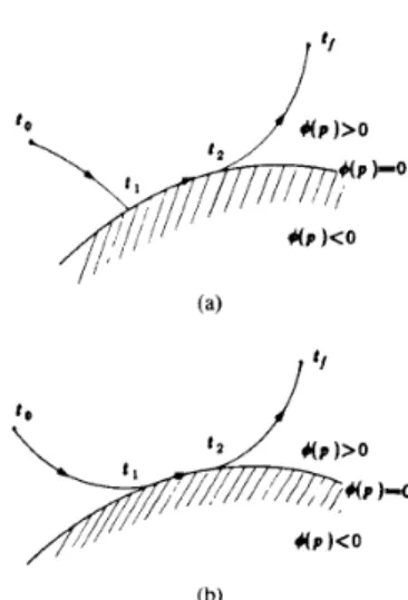
Fig. 2. Three-segment manipulator motion, t , = entry time, f2 = exit time. (a) Impact occurs at t I . (b) Impact does not occur at t , .

always directed toward the feasible region defined by the constraint. Equation (7) states that when the constraint is inactive, i.e., + ( p )

>

0 so that contact between the end effector and the constraint surface is not maintained, then X = 0 and thus f = 0. Equation (8) gives the impact relation, relating the manipulator velocities just before and just after

where the n-vectors p and q denote the end effector position vectors in Cartesian coordinates and joint coordinates; M(q) is the n x n inertial matrix; the n-vector function F(q, 4 ) is composed of a Coriolis term, a centrifugal term, and a gravitational term; the n-vector Tis the input joint torque; the m-vector h is the contact force multiplier; the n-vectorfis the contact force

and

are n x

n

and n x rn Jacobian matrices, respectively; ti is a transition time at which +(p(t))

>

0, ti- I

<

t

<

ti; $(p(t)) = 0 , ti I t I ti+ I ; t,? and t; denote the right-hand and left-hand

limits; and E represents the m-vector magnitude of a possible impulsive impact force.

Equation (2) is the dynamic equation of the manipulator; (3) is the contact force relation; (4) is the kinematic relation between the end effector position and the robot joint vector; (5) together with ( 6 ) and (7) are referred to as complementar-

ity conditions. Equation (6) implies that the contact force is

( 5 ) impact.

(6) (7)

The unilaterally constrained manipultor model consists of a set of differential equations and algebraic conditions. It has several features: i) two types of equations of motion of the manipulator system-when the manipulator end effector is not in contact with the constraint surface, the equations of motion of the manipulator are described by a set of differential equations; when the manipulator is in contact with the constraint surface, the equations of motion of the manipulator are governed by a singular system consisting of a set of differential and algebraic equations [2], [4], [5 ] ; ii) transition time-at which the manipulator transits from an unconstrained segment to a constrained segment, and vice versa: iii) impact issues-when the manipulator transits from an unconstrained segment to a constrained segment, impact is possible.

111. IMPACT CONDITIONS AND EXIT TIME

The entry time is a time at which the inactive constraint becomes active, e.g., t I in Fig. 2 denotes an entry time. When the manipulator transits from an unconstrained motion segment to a constrained motion segment at an entry time, there may exist an impact.

Assume there exists an impact at an entry time t l . We can derive an expression for the velocity of the end effector after impact. Two more assumptions are made:

(A4) The inertial matrix M(q) is nonsingular.

(A5) The Jacobian matrices D(H(q)) and J ( q ) are full rank. Since M(q) is invertible, we can solve for the velocity after impact q ( t : ) in terms of q ( t ; ) and

5 .

We have

(3)

Since D(p(tl))fi(t:) = 0 and the scalar A(q), defined by A. Path Planning A ( 4 ) = D ( f m ) ) J ( q ) M - ' ( 4 ) J T ( 4 ) D T W ( 4 ) )

is nonzero it follows that the magnitude of the impulsive impact force is

4

= - A -'(4(tl))D(P(tl))J(4(tl))q(t;)

= - A -'(4(tl))D(P(tl))P(t,). (10) Hence we obtain the following condition for avoidance of impact:

There is

no

impact

(E

= 0 ) i f and on& i f

D ( P ( t l ) ) f i ( t , ) = 0. (1 1) Thus an impact is avoided if the end effector of the manipulator comes to rest at t l , i.e., f i ( t ; ) = 0, or if the path of the end effector is tangent to the constraint surface at tl.

These two cases are considered separately in the subsequent formulation of optimal planning problems.

The exit time is a time at which the active constraint on the end effector becomes inactive, e.g., t2 in Fig. 2 denotes an exit time.

IV.

THE

PLANNING

PROBLEM

Our planning problem for a constrained manipulator is as follows: given the desired contact force, determine the joint input torques such that the manipulator is driven from a given initial configuration to a given final configuration, subject to satisfaction of i) constraints on the end effector motion, ii) impact avoidance, and iii) input torque constraints. If a cost criterion is imposed, then this problem becomes a minimum- cost planning problem or a so-called optimal planning problem. In general, an optimal planning problem can be formulated as an optimal control problem with constraints on state and control variables.

Optimization problems with equality and/or inequality state variable constraints have been extensively studied. These types of optimization problems are quite difficult to solve because the state variable constraints are infinite dimensional. Moreover, it is difficult to determine transition times at which constraints change between active and inactive.

In this paper, the optimization problem is simplified by a priori specification of the path of the end effector. We extend the method of Bobrow et al. [l] and Shin and McKay [7] to our optimal planning problem. Recall that the method of Bobrow et

al.

and

Shin

and McKay is based on a scalar parameterization of the path of the end effector which, in our

case, is chosen to guarantee satisfaction of the constraints.

This parameterization method reduces the dimensionality of the optimization problem from 2n to 2.

Our parameterized planning problem consists of three parts: 1) path planning-select a parameterization function P(s) so

thatp = P(s) satisfies the state constraints for 0 I s I

1;

2)

optimal motion planning-find a time optimal motion s = s(t) so that p ( t ) =

P(s(t))

for to I

t

I tf; 3 ) joint torque computation-compute the required joint torques from the manipulator dynamic equations.

We first need to select a suitable geometric path in the workspace of the manipulator to satisfy the constraints and other imposed requirements. We may regard path planning as one kind of spatial planning in the sense that the manipulator path is planned in the configuration space and the manipulator dynamics are not involved.

Let

P:

[0, 11

-,

R" be a parameterization function, where the variable s is referred to as a path variable. A kinematic approach is proposed to choose parameterization functions for the path. The kinematic approach is based on the satisfaction of the inequality constraint, the impact avoidance condition, and the boundary conditions. Recall that there are two unconstrained path segments: one is defined on 0 5 s

<

sl,

the other on s2

<

s 5 1.

During the constrained motion, the constraint r$(P(s)) = 0

must be satisfied for s1 I s I s2. Thus a selection of a parameterization function P(s), 0 5 s 5 1, should satisfy the following conditions:

W O )

=Po P(s1) =p1 cp(P(s))

>

0 O I S < S l (12)

+(P(s))

=

0

s1 I S I s2 P@2)=P2 W ) = P f r$(P(s))>O s 2 < s s 1 (14) where P(s) is continuous on [O, 11 and is twice continuously differentiable except possibly at s1 and s2.

Let Q: [0, 11 + R" satisfy

P(s)=H(Q(s)), 0 1 ~ 5 1. (15)

If the transformation H i s three times continuously differentiable, Q(s) possesses the same smoothness properties as P(s).

Thus we have the parametric representations

P =

P ( s )

4 =

Q(s).

(16)

For the first unconstrained path segment, the end effector of the manipulator makes contact with the constraint surface when s = sl. If

?Is1

lies in the tangent space of the constaint surface at s1 then no impact occurs at the entry time. This impact avoidance condition can be written as

wYsl))P'(sl) = 0 (17)

where

P'(s) =

-

.

as

(4)

HUANG AND MCCLAMROCH: ROBOTIC CONTOUR FOLLOWING PROBLEM ₁₄₃

B. Optimal Motion Planning

The second level of a parameterized manipulator planning problem is the optimal motion pianning problem. It can be stated as follows: given a path and the manipulator dynamics, determine the motion so that the manipulator moves along the prescribed path from the initial position to the final position in the shortest possible time. If a function

s:

[to, t,] + [O, 11 is

twice continuously differentiable and satisfies s(to) = 0, s(tf) = 1, then s(t) is referred to as a path history.

In this section, we first derive the equations of motion for a constrained manipulator along a parameterized curve. Then, a minimum-time planning problem for a constrained manipulator is formulated in two different ways according to the impact avoidance condition; in each case, a phase plane technique can be applied for its solution.

Suppose that the path of a manipulator is given by p = P(s), 0 5 s 5 1. We would like to derive the equations of motion of the manipulator along the prescribed path.

Assume the contact forceflt) is specified so that, according to (3), the multiplier A(t) is given by

In a time optimal problem, minimizing traversal time is equivalent to maximizing traversal speed. In fact, the minimum time solution consists of an accelerating part and a decelerating part; hence, limits on the path acceleration must

be considered. These limits are assumed to be imposed by the input joint torques

T.

For simplicity, the argument t is subsequently omitted throughout this subsection.

Let us consider constraints on the input joint torques of the form

T F ( q ,

q ) s q s T y ( q ,

q ) , i = l , e - . ,

n .

(23)

Since q is a function of s and q is a function of s and S, the torque constraints along the specified curve can be expressed in terms of s and 4 as

T?(s, S ) I ~ I T - ( S , S), i = l ,

.-.,

n.

(24)

Thus after algebraic manipulations, the path acceleration can

be shown to be constrained by functions of s and S, as

A(t) = A(s(t))u (S(t)), to I t I tf

(' 8, that is, the admissible path acceleration is constrained by (25).

We now obtain a single differential equation expressing s' in where A:[sl, sz] -+ RI is a known scalar function, and

terms of s, .S, .and T. From (20) .~ we obtain

9, _B

_T(s)B(s)s'

₊

_B

_'(s)l?(s)9

₊

_B

_T(s)M-

_{'(Q(s))F(Q(s),}

T = M ( Q (s)) B ( ~ ) s '

+

M ( Q

(s))

B

(s)S2

+

F(Q

-

J '(Q(s))D

'W(Q

(s)))Ns

1

(s) (2 1

1

or equivalently as

T ( t ) = T ( s ( t ) , S ( t ) , S'(t)). (22)

As long as s(t), S(t), and i ( t ) are known, the input joint torque

T(t) can be uniquely determined from (22).

1 ds

t f =

1:

1 d t =

-

.

o s

Thus the cost function for the three-motion-segment problem becomes

In the remainder of this section, we formulate a minimum- time motion planning problem; then we extend Bobrow and McKay's phase plane method so that it applies to the case of a constrained manipulator problem.

In order to guarantee the continuity of the velocity of the end effector at both the entry time and the exit time, additional conditions must be satisfied. The impact avoidance condition and the tangency condition can be written in parametric form

(5)

or

as Case 2: Suppose that the path function is selected so that it is differentiable and tangent to the constraint surface at the entry time and the exit time; then the impact avoidance condition and the tangency condition are automatically satisfied. The minimum time motion planning problem in this case becomes

D (P(s I))

J<Q

(si))B (si)$ (ti) = 0

W'(s2)) J(Q (s2))B (s2)S(t2) = 0.

(30) (31)

Given (27), the cost function in (29), and constraints (30)

and (31), we can formulate the minimum time motion planning

problem as follows. General Problem

Given a path p = P(s) and q = Q(s) satisfying (15) and

(16), find s(t), to I t I tf, the transition times tl and

t2,

the final tf, and the joint torque

T(t),

i = 1 ,

,

n

which minimize tfgiven by (29), subject to (27), the joint torque constraints (24), the impact avoidance condition (30), the tangency condition (31), and the boundary conditons s (0) =

0,

S(0)

= 0, s(tf) = 1 , S(tf> = 0, s(tl) = SI, and s(t2) = s2.

problem 2

Suppose that s1 and s2 satisfy D(P(sl)J(Q(sl))B(sl) = 0 and D(P(s2))J(Q(s2))B(s2) = 0. Given a pathp = P(s) and q = Q(s) satisfying (15) and (16), find s(t), to I t I tf9 the transition times ti and t2, the final time tf, and the joint torque T(t), i = 1 , * *

,

n

which minimize tfgiven by (29),

subject to (27), the joint torque constraints (241, and the boundary conditions s(0) = 0, S(0) = 0,

s(tf)

= 1

,

S(tr> =

o,

s(tl) = SI, and s(f2) = s2.

In this case, the end effector need not stop at the entry time and the exit time since the path speed is not constrained at these two instants. However, the path must be chosen so that s1 and

s 2 meet the requirements of (34) and (35). The resulting

minimum time planning problem for a constrained manipulator is a tractable minimum time planning problem without explicit state constraints.

This formulation guarantees that no impact occurs at the entry time, and that the end effector leaves the constraint surface tangentially at the exit time. As mentioned earlier, there are two ways to satisfy the impact avoidance condition and the tangency condition; they are to require that either

S(tl) = 0 (32)

S(t2) = 0 (33)

(34)

D (P(si)) J(Q (si))B (SI) = 0

o(P(sz))J(Q(s2))B(sz) = 0 (35)

where s1 = s(tl) and s2 = s(t2). Therefore, the minimum time motion planning problem can be reformulated in two different ways in terms of these two cases.

Case

I:

Suppose it is required that the end effector stops at the cntry time and the exit time so that S(tl) = 0, Q(t2) = 0.

The impact avoidance condition and the tangency condition are automatically satisfied. The minimum time planning problem becomes

C. Phase Plane Technique

of Minimum

Time Problem In the previous subsection, we have shown that the minimum time motion planning problem for a constrained manipulator can be reformulated as an equivalent minimum time motion planning problem without state variable constraints by properly choosing the parameterization function and including the desired contact force. The phase plane technique proposed by Bobrow [l] and McKay [6] can be

directly applied to these cases. We summarize that technique. The phase plane technique is based on the observation that to achieve minimum time control, the path acceleration 3 always takes its largest or its smallest possible values subject to satisfaction of (28). That is, finding the optimal time amounts to finding the times, or locations, at which s switches between maximum acceleration and maximum deceleration. The details have been given in [l], [6].

Now, we indicate how this phase plane technique can be applied to solve the optimal problems that have been devel- oped. In Case 1 , the minimum-time motion planning problem is divided into three uncoupled subproblems. Each subproblem is solved using the phase plane technique independently; then the results of the complete problem are obtained by piecing the results of the three subproblems together. In Case

2, the motion planning problem cannot be divided into several subproblems; it must be solved as a whole. The unconstrained motion segment and the constrained motion segment are governed by two different sets of equations of motion. When the phase plane technique is applied to this case, there likely occur discontinuities (e.g., cusps) in the boundary curve of the admissible region. Also the admissible region may become very complicated. These two features make application of the methodology more difficult, but the methodology discussed in

[l], [6] is still applicable to solve the minimum-time motion

Problem I

Given a path p = P(S) and

4

= Q(s) satisfying (15) and

(161, find s(t), to I t 5 tf, the transition times tl and t 2 , the

final time t f , and the joint torque

Ti

(0,

i = 1 , *

-

,

n

which

minimize tf given by (2% subject to (271, the Joint torque constraints (241, and the boundary conditions

s(0)

= 0, S(0)

= 0, s<tf) = 1 S(tf) = 0, s(tl) = SI, =

0,

df2) = s 2 , and S(t2) = 0.

Since the time optimal trajectory must satisfy S(tJ = 0 and S(t2) = 0 at the entry time and the exit time, respectively, we have the following result: The time optimal trajectory

of

Problem I can be accomplished by minimzing each motion segment independently.

Thus the total minimum traversal time of Problem 1 is equal to

tf= 71

+

7 2

+

7 3

where T ~ , 72, and 73 are the minimum times of the consecutive

(6)

HUANG AND MCCLAMROCH: ROBOTIC CONTOUR FOLLOWING PROBLEM 145

V. EXAMPLE CONTOUR FOLLOWING TASK problem description, we have

0.1303

A simple two degree-of-freedom Cartesian robot, such as a used

SIGMA to illustrate robot manufactured the contour by following the Italian task. company Olivetti, is

coordinates is denoted by p = (x,

v ) ~ .

For simplicity, we

[;]=[2]=[:::]

[::]=[1.0173]

The position vector of the end effector in planar workspace

assume that each link of the robot has a unit mass, and that

[ ;]

=

[

0.37163 1.1654 (3 9) gravitational, centrifugal, and Coriolis effects can be ne-

glected. Thus the open chain manipulator dynamics are given

x = F,

j = F y (36)

by

where F, and Fy are input joint forces. Assume the manipulator is to perform a contour following task on a constraint circle defined by

+ ( p ) = x 2 + (U- 1.5)2-0.25 2 0 . (37)

Consequently, the complete set of equations of motion used to describe the contour following task is obtained as and

2 = F,+ 2xX

As mentioned previously, the path can be chosen to satisfy the impact avoidance condition. Two different choices of the path function are considered.

Path with Discontinuous Slopes at the Entry and the Exit Time: In this case, the path is chosen to satisfy the boundary conditions

WO,

YO), ( X I , YI), ( X Z , YZ), (xf,

ur);

the normality condition [x’(s)]’

+

Iy’(s)]* - 1 = 0,O I s I 1;

and the constraint x2(s)

+

Iy(s)

-

1.512

-

0.25 1 0, O r

s

r 1; where

j;=Fy+2(y- 1.5)h

We can adjust

sI

and sz so that the normality condition is satisfied. After some computation, the path is obtained as follows:

A20

x2

+

(U

- 1 .5)2

-

0.25 2 0 X[X*+(Y- 1.5)2-0.25] = O x ( s ) = al s

+

a2 y

(s)

=

a3s

+

a4, 0 5 s

<

s, (40) X(t’) = a @ : ) +2X(ti)I _{X ( S ) =}_0.5_COS_(2s_-₂₎

Y(t,?) = j ( t 1 7 )

+

2 [ y ( t j ) - 1.5][ (38) y ( s ) = 1.5+0.5 sin (2~7-2)~ SISSSSZ (41)

where

X

is the contact force, ti is the entry time, and is the magnitude of the possible impulsive impact force. Now a contour following task can be stated as follows:

The end effector of the manipulator is initially at rest at position (x, y) = (0.4, 0.8). With the manipulator dynamics defined in (38), the end effector is to move from the initial position (x, y ) = (0.4, 0.8) and contact the constraint at position (x, y) = (0.1303, 1.0173). Then, the end effector is to follow the constraint in the counter clockwise direction with a specified constant contact force,

X

= 1 , to another point on the constraint (x, y ) = (0.3716, 1.1654). Finally, the end effector leaves the constraint and moves back to the starting point.

Given this example contour following problem, path planning and time optimal motion planning issues are discussed in the next subsection.

A. Path Planning

Let PT(s) = [x(s), y(s)] denote the parameterization =

[xf,

yf] denote the initial point, the entry point, the exit point, and the final point, respectively. According to the function, and P; =

Bo,

Yo19

P;

= [XI, A I , Pz’ = 1x2,

yd,

P;

x ( s ) = CIS+ c2 y(s)=c3s+c4, S Z < S I 1 (42) where S I = 0.3464 ~2 = 0.6335 al =

-

0.7788

a3

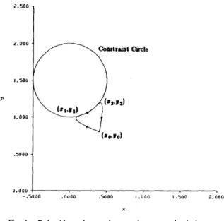
= 0.6273 a2 = 0.4 a4 = 0.8 CI = 0.0776 CZ = 0.3224 ~ 3 = -0.997 ~ 4 = 1.797. (43)

The desired path and constraint are shown in Fig. 3. Points

(xo, yo), ( X I ,

U]),

and (x2, y2) denote the initial point, the entry point, and the exit point, respectively. The slope of the path is discontinuous at the entry point and the exit point.

Path with Continuous Slope: In this case, the path is chosen to satisfy the boundary conditions (XO, YO), (XI, V I ) , ( X Z ,

y2), (xf, y f ) ; the impact avoidance condition at sl, x(sl)x’ (sl)

+

[y(s,)

-

1.5 ]U’

(sI)

= 0; the tangency condition at s2,

(7)

2 . 5 0 0 - .5000

{

0 . 0 0 0 4 -.5000 .OUOO .5000 1.000 1.500 2.000

I

2.500 2.000 .5000 - o.aoo 4 -.5000 . D O 0 0 .5UOO 1.0011 1.500 2 . 0 0 0 x X

Fig. 3. Path with discontinuous slopes at the entry and exit times. Fig. 4. Path with continuous slopes at the entry and exit times.

x2(s)

+

[y(s)

-

1.512

-

0.25 1 0, 0 I s 5 1 . In order that the path is tangent to the constraint at the entry time and the exit time, two more conditions must be satisfied:

and

After some computation, the path is obtained as follows:

~ ( ~ ) = d l s ~ + d z s + d 3

Y ( S ) = d4s2

+

d 5 ~

+

d6, O S S < S ~ (44)

x ( s ) = O . ~ COS (2s-2)

y(s)=1.5+0.5 sin (2s-2), s l ~ s ~ s 2 (45)

x ( s ) = e I s 2

+

e2s

+

e3

y(s) = e4s2

+

e5s+ e6, s2<sc 1 (46)

where SI = 0.3464 dl = 5.036 d2= -2.5231 d3=0.4 ~2 = 0.6335 d4=

-

1.0589 ds = 0.994 d6 = 0.8 el = - 1 A14 e4 = - 4.7475 e5 = 6.758 e6=

-

1.2104. (47) e2 = 2.7139 e3 =

-

0.7

The desired path and constraint circle are shown in Fig. 4.

Points (xo, yo), (xl, yl), and (xz, y2) denote the initial point, the

entry point, and the exit point, respectively. The slope of the path is continuous at the entry point and the exit point.

B. Optimal Motion Planning

The optimal motion planning can be formulated in two ways according to satisfaction of the impact avoidance conditions:

1) the end effector comes to rest at both the entry time and the exit time, 2) the path is tangent to the constraint at both the entry time and the exit time. In each case, a minimum-time motion planning is discussed.

Case I: S(t) = 0 and

S(t2)

= 0: In this case, the end effector comes to rest at both the entry time and the exit time. Hence,

no impact occurs at the entry time tl. Equations (40) and (43)

are used to generate the desired path for motion planning. With the above information, the joint forces F, and Fy can be

obtained by

F,=als

Fy=a3s, O I S < S ~ (48)

F,=

-

sin (2s

-

2)s’- 2S2 cos (2s

-

2)

-

cos (2s

-

2) Fy = cos (2s

-

2)s’- 2S2 sin (2s

-

2) - sin

(2s

-

2),

SI 5 s 5 s 2 (49)

F,= CIS

FY=c~S, S ~ < S S 1 (50) where ai, ci, and SI, s2 are given in (43).

In this minimum-time approach, the entry time t l , the exit time t2, the final time tf, the path history s(t), and the joint forces F,, Fy are to be determined so that the boundary conditions s(0) = 0, S(0) = 0 , s(tl) = sl, S(tl) = 0 , s(t2) =

s2, S(t2) = 0 , s(t’) = 1 , S(tf) = 0 are satisfied, and the following joint force constraints:

(8)

HUANG AND MCCLAMROCH: ROBOTIC CONTOUR FOLLOWING PROBLEM 1 r d ) e c l O r ~

-

boundary --- .7000 . W O .L(zoo - U .2000 . 1 w o 0 . 0 0 0 S

Fig. 5. Phase plan plot of minimum-time approach with Fig. 3 path. are satisfied and

tf

is a minimum. The single equation for

s'

is obtained as

alF,+ a3Fy, 0 5 S < S l

CIF,+ c3Fy, s2<s51

s= -sin (2s-2)FX+cos (2s-2)Fy, sl-Csls2

(52)

t

where relations a:

+

4

= 1 and c:

+

c$ = 1 , are used; a l , a3, cI, c3, SI, s2, are given in (43). From the discussion in Section

IV,

the minimum-time motion planning problem for this case can be divided into three subproblems. The phase plane technique can be used to solve these three subproblems; we obtain

71= 1.0383 s 7 2 ~ 2 . 4 3 3 3 s 73= 1.2014 s

where 71 denotes the cost function of the minimum-time

. . - -

-

.

"

subproblem for U I s

<

sl, 7 2 for s1 I s I s2, and 73 tor s2

<

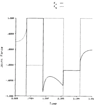
s I 1 . The complete phase plane trajectory and inadmissible region are shown in Fig. 5 . The trajectory passes through points (0.3464,O) and (0.6335,O). This shows that the end effector comes to rest at the entry time and the exit time. Note that an inadmissible region exists only for the constrained motion; there are no inadmissible regions for the unconstrained motion segments; there are no inadmissible regions for the unconstrained motion segments for this particular example. In addition, the phase plane trajectory never touches the inadmissible region. There is only one switching point for each motion segment. The optimal joint forces F, and Fy are shown in Fig. 6 . The joint forces are discontinuous not only at the entry time and the exit time but also at each switching point.

Case 2: S ( t l ) # 0 and S(t2) # 0: In this case, the path is

I. 000 .bo00 $ .2000

c

L 0 LL 4 0 - . P O 0 0 7 - . 6 0 0 0 -1.000 0 F *

-

FU ---

I

A .9N6 1.069 2.80q 3.738 Y.673 Time

Fig. 6. Joint force plot of minimum-time approach with Fig. 3 path. chosen to satisfy the impact avoidance condition so that

no

impact occurs at the entry time

t l .

Equations

(44)

and (47) are used to generate the desired path for motion planning. With the above information, the joint forces F, and Fy can be

obtained by

FX=(2dls+d2)S+2dlS2

Fy = (2d4s

+

d5)s'+ 2d4S2,

0

Is<s~

F, =

-

sin (2s

-

2)3

-

2S2 cos (2s

-

2)

-

cos (2s

-

2) Fy = cos (2s

-

2)3- 2S2 sin (2s

-

2) - sin (2s

-

2),

(53)

S , I S I S 2 (54)

F,=(2els+e2)3+2elS2

Fy=(2e4s+e5)3+2e4S2, s2<sC 1 ( 5 5 ) where di, ei, and SI, 52 are given in (47).

In this minimum-the approach, the entry time

t l ,

the exit time

tz,

the final time

tf,

the path history s(t), and the joint forces F,, Fy

are

to be determined so that the boundary conditions s(0) = 0, S(0) =

0,

s(tl)

= sl, s(t2) = s2,

s(tf)

=

1, S(tf) = 0, and the joint force constraints (51) are satisfied and

tf

is a minimum. The single equation for s' is obtained as

(2d1s+ dZ)(F,- 2d1S2)

+

(2d4s+ d5)(Fy

-

2d4S2)

O I S < S , ~1 I S I ~2 (56)

(2dIs

+

d2)2

+

(2d4s

+

d J 2 9

-

sin (2s

-

2)F,

+

cos (2s

-

2)F,,

(2els

+

e&F,

-

2elS2)

+

(2e4s

+

e5)(F,

-

2e4S2) (2els

+

e2)2

+

(2e4s

+

e5)2 9

(9)

148 .W67 .7253 . 5 W O *U) .362 7 .I813 0 . 0 0 0 0.

IEEE JOURNAL OF ROBOTICS AND AUTOMATION, VOL. 4, NO. 2, APRIL 1988

t r a j e c ~ o r y

-

boundary

---

I.001 .6OOC $ .2ooa L 0 L L L

c

0 -.PO00 7 -.6000 0 .2000 .qooo .6000 .EO00 1.000 5

Fig. 7. Phase plane plot of minimum-time approach with Fig. 4 path.

where

di,

ei,

sl,

and

s2

are given in (47). From the discussion in Section IV, the minimum-time motion planning problem for this case must be treated as a whole. The phase plane technique can be applied to solve this problem, resulting in

tfz3.992 s tlz1.4285 s t2=2.492 s

where s(tJ = s1 = 0.3464, and s(t2) = s2 = 0.6335. The complete phase plane trajectory and inadmissible region are shown in Fig. 7. The boundary curve is denoted in dashed line. There are two cusps and two jumps in the boundary curve. The resulting trajectory has six switching points. The joint forces F, and Fy are shown in Fig. 8.

C. Remarks

If the end effector comes to rest at the entry time and the exit time, the total minimum traversal time (Case 1) is 4.673

s.

On the other hand, if the end effector does not stop at the entry time and the exit time, the minimum traversal time (Case 2) is reduced to 3.992 s.

VI. CONCLUSION

A robotic contour following problem, defined by a unilaterally constrained manipulator, has been presented. Our approach differs from previous approaches in that our approach explicitly takes into account inequality constraints and resulting contact forces as part of the system dynamics. Possible impact at an entry time is also discussed. A parameterization approach to select a suitable path function has been applied to planning for the contour following problem. The minimum- time motion planning problem has been reformulated so that a phase plane technique can be applied. The desired contact force is incorporated in the optimal planning scheme.

Finally, an example contour following task has been used to illustrate the ideas developed in this paper. The results are

-1.000 F x

-

F,, - - - . _ _ _ _ _ _ _ _ _ _ _ _ _ _ _ ,

/--

I 0.000 . 7 9 w 1.597 2.395 3.1911 3.992 T i m e

Joint force plot of minimum-time appraoch with Fig. 4 path. Fig. 8.

quite satisfactory. Although the manipulator used in the example is a simple Cartesian robot, the devloped theory is, in principle, applicable to other robot configurations and other constraints.

In this paper, friction on the constraint surface and multiple inequality constraints have not been discussed. The contact force and the path of the end effector in the optimal planning formulation have been specified

a

priori rather than determined by the optimal planning procedure. These assumptions are very important. The extensions are nontrivial. This paper should provide a basis for further developments for constrained manipulators and robotic contour following problems.

I11

P I

r31 [41 I51 I61 r71 181 r91 REFERENCES

J. E. Bobrow, et al., “Time optimal control of robotic manipulators along specified paths,” Int. J. Robotics Res., vol. 4, no. 3, Fall 1985, S. L. Campbell, Singular Systems of Differential Equations II. San Francisco, CA: Pitman Advanced Publ. Program 1982. H. P. Huang, “Constmined manipulators and contact force control of contour following problems,” Ph.D. dissertation, Dep. of Electrical Engineering and Computer Science, The University of Michigan, July 1986.

N. H. McClamroch and H. P. Huang, “Dynamics of a closed chain manipulator,” presented at the American Control Conf., Boston, MA, June 1985.

N. H. McClamroch, “Singular systems of differential equations as dynamical models for constrained robot sytems,” presented at the 1986 IEEE Robotics and Automation Conf., San Fransciso, CA. Apr. 1986. N. D. McKay, “Minimum-cost control of robotic manipulators with geometric path constraints,” Ph.D. dissertation, Dep. of Electrical Engineering and Computer Science, The University of Michigan, Oct. 1985.

K. G. Shin and N. D. McKay, “Minimum-time control of robotic manipulators with geometric path constraints,” IEEE Trans. Auto- mat. Contr., vol. AC-30, no. 6, pp. 531-541, June 1985. G. P. Starr, “Edge-following with a PUMA 560 manipulator using VAL-11,” presented at the 1986 IEEE Robotics and Automation Conf. D. E. Whitney, and A. C. Edsall, “Modeling robot contour proc- esses,” presented at the American Control Conf., June 1984.

(10)

HUANG AND MCCLAMROCH: ROBOTIC CONTOUR FOLLOWING PROBLEM 149 Han-Pang Huang (S’83-M’86) was born in Nan- N. Harris McClsmroch (M’67-SM’86-F’88) re- tou, Taiwan, R.O.C., on October 7, 1956. He ceived the B.S. and M.S. degrees in mechanical received the Diploma in electronic engineering from engineering and the Ph.D. degree in engineering Taipei Institute of Technology, Taipei, Taiwan, in mechanics, all from The University of Texas,

1977, and the M.S. and Ph.D. degrees in electrical Austin, in 1963, 1965, 1967, respectively. engineering from The University of Michigan, Ann Since 1967 he has been at The University of Arbor, in 1982 and 1986, respectively. Michigan, Ann Arbor, where he is currently a From 1977 to 1979 he was a reserved officer in Professor in the Department of Aerospace Engi- the Chinese Air Force; from 1979 to 1981 he served neering; he also holds a joint appointment with the as a senior technician in the Taipei Long Distance Department of Electrical Engineering and Com- Telecommunication Office; from 1982 to 1986 he puter Science. His research interests are in the area held a research assistant in the Center for Research and Integrated Manufac- of stability and control of nonlinear feedback systems, and include applica- turing, The University of Michigan. In 1986, he joined the Department of tions to control of mechanical systems. He is the author of more than sixty Mechanical Engineering, National Taiwan University, Taipei, Taiwan, as an technical papers and one book, StuteModels of Dynamic Systems: A Case associate professor. His research interests include constrained robots, Study Approach. He is currently the Associate Editor for the IEEE machine intelligence, control of singular system, and adaptive control. TRANSACTIONS ON AUTOMATIC CONTROL with responsibility for

technical notes and correspondence. Dr. Huang is a member of SME/RI and Tau Beta Pi.