適用於長程演進網路上行傳輸之預測式資源排程法

國

立

交

通

大

學

網路工程研究所

碩

士

論

文

適用於長程演進網路上行傳輸之預測式資源排程法

An Estimation Based Resource Allocation Algorithm for LTE Uplink

Transmission

研 究 生：張家愷

指導教授：趙禧綠 教授

適用於長程演進網路上行傳輸之預測式資源排程法

An Estimation Based Resource Allocation Algorithm for LTE Uplink

Transmission

研 究 生：張家愷 Student：Chia-Kai Chang

指導教授：趙禧綠 Advisor：His-Lu Chao

國 立 交 通 大 學

網 路 工 程 研 究 所

碩 士 論 文

A Thesis

Submitted to Institute of Network Engineering College of Computer Science

National Chiao Tung University in partial Fulfillment of the Requirements

for the Degree of Master

in

Computer Science

July 2012

Hsinchu, Taiwan, Republic of China

I

適用於長程演進網路上行傳輸之預測式資源排程演算法

學生：張家愷 指導教授：趙禧綠博士

國立交通大學資訊學院網路工程研究所

摘要

長期演進技術(LTE)為第三代合作夥伴計劃(3GPP)制定之標準，並且被公認為是邁 向 4G 網路時期的一項很有前景的科技。由於在下行鏈路中使用正交分頻多工存取 (OFDMA)技術，以及在上行鏈路中使用單載波分頻多工存取(SC-FDMA)技術，因此 LTE 相較於 3G 網路可以在頻寬最高 20MHz 上面提供極高的傳輸速率。 為了增加基地台的整體傳輸速率與使用者多樣性增益之目的， LTE 在以 OFDMA 為技術的下行鏈路中是採納傳統的通道相依排程演算法(CDS)。CDS 演算法會優先將各 個資源區塊(RB)各別的配置給在這個 RB 頻道品質較好的使用者，然而這個方法若同樣 的套用在以 SC-FDMA 為技術的上行鏈路中，則可能會讓整體的傳輸表現變得不盡理想。 會發生這個問題的主要原因是因為 SC-FDMA 技術比 OFDMA 技術在配置資源的時候多 了兩個限制，第一個是使用者在配置資源時必須符合連續限制，第二個則是針對一個使 用者在所有被配置的 RBs 都必須使用相同的調變技術(MCS)。此次論文將把目標鎖定在 探討上行鏈路以 SC-FDMA 為技術的排程演算法。由於上行鏈路的資源配置最佳解已經 被証明為 NP-hard 問題，因此我們將藉由提出新的概念以發展出一個啟發式演算法，並 且嘗試去逼近問題的最佳解。最後將以模擬評估本論文提出之演算法，結果顯示此方法 在系統總傳輸率相較於傳統以 CDS 為基礎的方法有明顯的改善。

II

An Estimation Based Resource Allocation Algorithm for

LTE Uplink Transmission

Student: Chia-Kai Chang Advisor: Dr. Hsi-Lu Chao

Institute of Network Engineering College of Computer Science National Chiao Tung University

Abstract

Long Term Evolution (LTE) is a promising technology for 4G mobile networks standard by 3rd Generation Partnership Project (3GPP). Due to utilize OFDMA in downlink and SC-FDMA in uplink, the LTE system is expected to provide significantly high throughput with 20 MHz spectrum allocation compared to 3G mobile networks.

To increase the cell throughput and multi-user diversity gain, Channel Dependent Scheduling (CDS) is implemented for the OFDMA-based multi-user scenario to allocate Resource Blocks (RBs) to users experiencing better channel conditions. Nevertheless, CDS may not perform well in SC-FDMA due to its two inherent constraints－one is contiguous RB assignment and the other is robust Modulation and Coding Scheme (MCS). In this thesis, since the optimization problem of resource allocation in SC-FDMA is NP-hard, we hence propose an estimation-based heuristic algorithm, which will take the two inherent constraints of SC-FDMA into consideration. In the algorithm, each time it will try to allocate one RB to the User Equipment (UE), which can maximize the current upper bound estimation. We evaluate the proposed algorithm by conducting simulation. The simulation results show that our method can achieve significant performance improvement in system throughput.

III

誌謝

兩年的時間過去了，開始寫論文和準備口試的日子也到來了。在碩士的求學時光裡， 很開心能夠克服種種的考驗、困難與挫折，並且不斷的努力鞭策自我，致使自己能夠順 利的完成課業和論文，準備畢業的到來。 首先，很感謝家裡的支持。即使家愷在國中和高中曾經沉迷於遊戲世界而不斷的想 要放棄學業，家庭總是不斷的在背後默默的體諒、鼓勵和從旁協助，因此也讓我可以將 從前不快樂的各種事情拋諸腦後，努力的往上學習。很高興自己終於到了畢業的時間， 終究沒有辜負了家裡的培養。 家愷也很感謝我的指導老師，趙禧綠教授。在碩零期間，老師告訴了我們實驗室的 方向，並且讓我們可以開始研讀自己有興趣的論文以尋找未來的研究題目。碩一修習課 業、確定題目，碩二的論文研究、會議投稿、計畫申請、專利撰寫，到論文的正式完成 和口試準備，老師在各個方面總是不斷的從旁給予協助和鼓勵，並且告知家愷正確的方 向。 另外，我也要感謝實驗室裡的學長姐、同學以及學弟妹們。在家愷對於研究的知識 不足的時候，學長姐總是會很熱心為我解答，並且告知哪邊會有我需要的文件。同學們 總是在家愷心煩意亂的時候，很有義氣的陪我一起出去玩樂解悶，並且幫忙想辦法解決。 碩一暑假的墾丁旅行雖然很不巧的遇到颱風，但是能夠跟大家一起郊遊實在是很難忘的 經驗。而每星期的籃球運動也讓大家除了可以多多活動筋骨之外，更可以凝聚實驗室的 向心力。 最後我要感謝交通大學給了我們一切的資源。實驗室和會議室，讓家愷可以努力的 作研究和報告。不論是研究相關或課外書籍，圖書館提供了我們龐大的書籍資料。也很 謝謝體育室提供家愷設備新穎的健身房和游泳池，讓我在研究疲憊之於，能夠藉由運動 抒發壓力。 畢業的時間到了，也到了面臨兵役和工作的時候了。在工作之後，家愷會將這兩年 從交通大學所學到的知識貢獻予社會，期望能夠在這個競爭激烈的世界中有所成就。而 家愷也會將工作後得到的資源給予學校，讓交通大學可以不斷的提升競爭力並且培養出 更多的卓越學生。在這，我要謝謝所有的家人、老師、同學和學校，謝謝各位一路的栽 培與相挺。

IV

Contents

摘 要……….I Abstract ………..II 誌 謝 ... III Contents………...…….IV Lists of Table ... V Lists of Figure ... VI Chapter 1 Introduction ... 1

1.1 Resource Block and Scheduling Procedure ... 2

1.2 Problem Statement ... 5

1.3 Organization ... 7

Chapter 2 Related Work ... 8

Chapter 3 Proposed Algorithm ... 13

3.1 System Model ... 13 3.2 Problem Formulation ... 13 3.3 Heuristic Method ... 18 3.3.1. Brief Introduction ... 19 3.3.2. Method Description ... 20 3.3.3. Detailed Example ... 27

3.3.4. Pseudo Code ant Time Complexity ... 33

Chapter 4 Simulation Results ... 41

4.1 System Throughput ... 42

4.2 Starvation Ratio ... 45

4.3 Influence of Window Size ... 47

4.4 Problem of UBERA ... 49

Chapter 5 Conclusion ... 50

V

Lists of Table

Table I. The definition of parameters in problem formulation ... 15

Table II. The mapping table from SNR threshold to MCS ... 17

Table III. Example – Initial SNR table ... 27

Table IV. Example – Build window SNR table ... 28

Table V. Example – Choose starting RB to UE ... 29

Table VI. Example – Adjust SNR table ... 30

Table VII Example – Adjust window SNR table ... 31

Table VIII Example – Choose next RB ... 31

Table IX Example – Choose available allocated UEs ... 32

Table X Example – Upper bound estimation ... 33

Table XI Example – Scheduling result ... 33

Table XII Pseudo code of UBERA ... 34

Table XIII Pseudo code of Adjust SNR table ... 37

Table XIV Pseudo code of Adjust window SNR table ... 38

VI

Lists of Figure

Figure 1. Time domain view of the LTE ... 2

Figure 2. Time and frequency domain – user scheduling ... 3

Figure 3. Constraint of LTE UL resource allocation ... 5

Figure 4. Effect of choosing first RB to UE ... 6

Figure 5. Matrix algorithm and Search-tree based algorithm ... 9

Figure 6. The resource allocation results of RME, FME and MADE ... 9

Figure 7. IRME and ITRME ... 11

Figure 8. An illustration of parameter definition ... 15

Figure 9. The flowchart of UBERA ... 20

Figure 10. System throughput with optimum solution be compared ... 43

Figure 11. System throughput without optimum solution be compared ... 44

Figure 12. System throughput with different fading channel ... 45

Figure 13. Starvation ratio vs. Number of UEs ... 46

Figure 14. System throughput with different window size ... 47

1

Chapter 1 Introduction

The Long Term Evolution (LTE), marketed as 4G LTE, is one of important standard for wireless communication. The standard is developed by the 3rd Generation Partnership Project (3GPP), which is specified in 3GPP’s Release 8 documents frozen in December 2008 with minor enhancement specified in Release 9 documents frozen in December 2009. With the reduced latency (5ms for small packet and 100ms for device wake up), higher data rate (peak data rate 300 Mbps for downlink while 75 Mbps for uplink for system bandwidth 20MHz and UE Category 5), flexible spectral usage (1.4, 3, 5, 10, 15, 20MHz with TDD and FDD available), better performance with high mobility equipment (maximum to 350km/h) and spatial multiplexing supported (single layer for Uplink (UL) per User Equipment (UE), up to 4 layers for Downlink (DL) per UE, and MU-MIMO supports for UL and DL), LTE is well-prepared to meet user expectation in a 10-year perspective and beyond [1].

To achieve these objectives, Orthogonal Frequency Division Multiple Access (OFDMA) has been selected as the DL access scheme for LTE cellular systems. Rather than transmitting a high-rate stream of data with a single carrier, OFDM makes use of a large number of closely spaced orthogonal subcarriers that are transmitted in parallel. Each subcarrier is modulated with a conventional modulation scheme (such as QPSK, 16QAM, or 64QAM) at a low symbol rate [2]. However, OFDMA is not suitable for the UL access scheme due to high Peak-to-Average Power Ratio (PAPR) which will shorten battery lifetime at User Equipment (UE), and leads 3GPP to look for a different transmission scheme for the LTE UL. Therefore, another modulation scheme－Single Carrier Frequency Division Multiple Access (SC-FDMA), is adopted for LTE UL transmission. Comparing to OFDMA, SC-FDMA performs a Discrete Fourier Transform (DFT) prior to the conventional Inverse Fast Fourier Transform (IFFT) operations, which spreads the data symbols over all the subcarriers and produces a virtual single-carrier structure [3]. This modification not only reduces consumed power significantly,

2

but also keeps the inherent advantages of OFDMA such as high spectral efficiency and robustness to multipath fading.

1.1 Resource Block and Scheduling Procedure

Figure 1. Time domain view of the LTE [4]

The time domain view and physical layer resource structure of LTE specified by 3GPP is shown in Fig. 1. As to time domain, a full frame is 10 ms but we normally think in terms of the 1 ms sub-frame, which is the entity that contains the Transport Block (TB). Within the TB (MAC PDU) are the MAC header, MAC SDUs and padding. Within the MAC SDU (RLC

3

PDU) are the RLC header and RLC SDUs, then within the RLC SDU (PDCP PDU) there can be a number of PDCP SDU IP Packets coming from network layer [4]. As to physical layer resource structure, the spectrum is divided into Resource Blocks (RBs), where a TB will be loaded into a number of RBs by scheduler at eNodeB. The number of RBs to load the specific TB is decided by the data size of TB and the data size can be loaded of single RB. RB is the basic LTE resource unit, which is a two dimensional rectangle wrapped by 12 adjacent spaced 15 kHz subcarriers in frequency domain and either 6 or 7 OFDM symbols in time domain depends on the Cyclic Prefix (CP). When a normal CP is used, the RB contains 7 symbols. When an extended CP is used, the RB contains 6 symbols. Two RBs consecutive in time domain form a single Scheduling Block (SB), which is the basic unit of bandwidth to be allocated to specific TB. The duration of SB equals the length of a sub-frame and represents a scheduling period, named Transmission Time Interval (TTI) [5]. In the latter of thesis, allocating single RB represents two time consecutive RBs of single SB. Besides, the smallest modulation structure in LTE is the Resource Element (RE). A RE is wrapped by one 15 kHz subcarrier and one OFDM symbol, which can carry several data bits depending on the adopted Modulation and Coding Scheme (MCS) mode. Since RB is composed of several REs as shown in Fig. 1, which is the smallest allocated unit, we define the sum data bits of a RB as “RB capacity”.

4

As active UE tries to request UL transmission resources from eNodeB, the UE uses Scheduling Request (SR) mechanism, which conveys a single bit of information indicating the UE has new data to transmit. The SR mechanism can be either Dedicated-SR (D-SR) or Random Access-based SR (RA-SR). While the UL of the UE is not time aligned or no Physical Uplink Control Channel (PUCCH) resources for D-SR are assigned to the UE, RA-SR must be used to (re-)establish time alignment. If the time is aligned and PUCCH resources are assigned, D-SR can be conveyed on PUCCH. After SR mechanism, portion of Physical Uplink Shared Channel (PUSCH) resources will be allocated to the UE. Then the Buffer Status Report (BSR) about the amount of data waiting in the UE is attached to the first UL transmission following the SR procedure on allocated PUSCH resources. After getting BSRs from UEs, the Packet Scheduler (PS) at eNodeB in each TTI makes decision on allocating RBs according to Sounding Reference Signals (SRSs) from all UEs. The SRS is a known sequence transmitted by UE periodically, where the UE-specific periodicity can be 2 / 5 / 10 / 20 / 40 / 80 / 160 / 320 ms as defined in [7] section 8.2. Getting SRS sequences from UEs, the SRSs are used at the eNodeB to extract the instantaneous Channel State Information (CSI) of the RBs of UEs, in which the CSI function is similar to the Channel Quality Indicator (CQI) in DL [8]. The better CSI of a RB refers to the higher RB capacity can achieve. Since the channel conditions are distinct among different RBs and uncorrelated for different UEs, PS will assign UE a portion of bandwidth that is in its favorite conditions. After PS decides resource allocation of UEs as illustrated in Fig. 2, eNodeB conveys UEs using Downlink Control Information (DCI) on Physical Downlink Control Channel (PDCCH). DCI contains information indicating MCS to be used and number of allocated RBs. Besides, DCI also tells the index of starting RB of UL resource allocation as well as number of contiguously allocated RBs.

5

1.2 Problem Statement

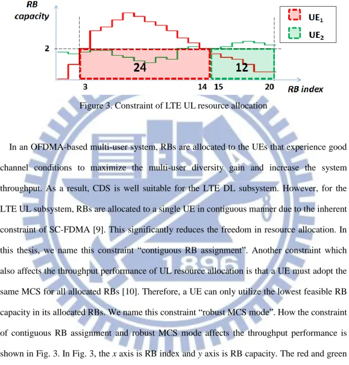
Figure 3. Constraint of LTE UL resource allocation

In an OFDMA-based multi-user system, RBs are allocated to the UEs that experience good channel conditions to maximize the multi-user diversity gain and increase the system throughput. As a result, CDS is well suitable for the LTE DL subsystem. However, for the LTE UL subsystem, RBs are allocated to a single UE in contiguous manner due to the inherent constraint of SC-FDMA [9]. This significantly reduces the freedom in resource allocation. In this thesis, we name this constraint “contiguous RB assignment”. Another constraint which also affects the throughput performance of UL resource allocation is that a UE must adopt the same MCS for all allocated RBs [10]. Therefore, a UE can only utilize the lowest feasible RB capacity in its allocated RBs. We name this constraint “robust MCS mode”. How the constraint of contiguous RB assignment and robust MCS mode affects the throughput performance is shown in Fig. 3. In Fig. 3, the x axis is RB index and y axis is RB capacity. The red and green curves are the envelope of the RB capacity for UE1 and UE2 for all observed RBs, respectively. For the constraint of contiguous RB assignment, we can see that the UEs must get RBs in the contiguous frequency band. On the other hand, for the constraint of robust MCS mode, we can see that even UE1 has good RB capacity in the middle of its allocated RBs, these RBs’ capacity must be slowed to the RB capacity of RB3. Here, RB3~RB14 are allocated to UE1 and

6

RB15~RB20 are allocated to UE2. RB1 and RB2 are unused. The system throughput performance of this example is 2*(20-3+1) = 36. However, it is easy to get better system throughput by allocating RB4~RB12 to UE1 and RB13~RB20 to UE2, where the system throughput promotes to 43.

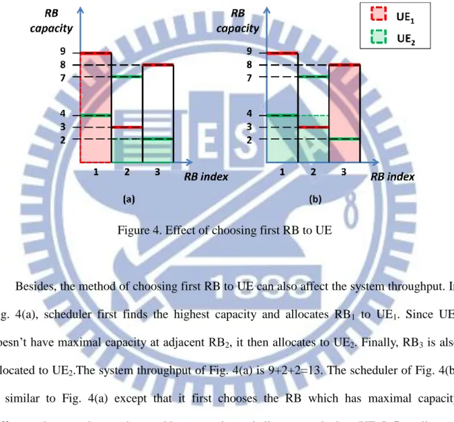
Figure 4. Effect of choosing first RB to UE

Besides, the method of choosing first RB to UE can also affect the system throughput. In Fig. 4(a), scheduler first finds the highest capacity and allocates RB1 to UE1. Since UE1 doesn’t have maximal capacity at adjacent RB2, it then allocates to UE2. Finally, RB3 is also allocated to UE2.The system throughput of Fig. 4(a) is 9+2+2=13. The scheduler of Fig. 4(b) is similar to Fig. 4(a) except that it first chooses the RB which has maximal capacity difference between best and second best capacity and allocates to the best UE. It first allocates RB3 to UE1.Then RB1 and RB2 are allocated to UE2. The system throughput of Fig. 4(b) is 4+4+8=16. Thus it tells the CDS which greedily allocates RB to the best UE may not work well in SC-FDMA.

7

1.3 Organization

The remainder of the thesis is organized as follows. Related works are mentioned in chapter 2. The system model of LTE UL subsystem and the problem formulation are presented in chapter 3.1 and 3.2, respectively. The method description, detailed example, time complexity analysis and pseudo code of proposed estimation-based resource allocation algorithm are described in the remainder of chapter 3. The performance evaluation results are presented and discussed in chapter 4. Finally, the conclusions and future work are described in chapter 5.

8

Chapter 2 Related Work

There are many works focused on LTE DL resource allocation [11][12][13][14][15], and these proposed methods indeed have great improvement on system throughput performance. However, these methods cannot be applied to LTE UL resource allocation directly due to the constraint of “contiguous RB assignment.” Hence, there exists many works focused on improving system throughput of LTE UL. In this chapter, we first investigate methods of these LTE UL resource allocation works, and a summary is mentioned in the end of this chapter.

Calabrese et al. in [16] propose a search-tree based algorithm. At first, the authors divide the system bandwidth into Resource Chunks (RCs), which are equal sized and constituted by a set of consecutive RBs. The size of the RC is chosen to be a sub-multiple of the system bandwidth so that an integer number of UEs can be accommodated without creating bandwidth fragmentation. In algorithm description, this paper first described matrix algorithm, which continually allocates RC to UE with the highest metric. The author points the approach can provide significant gain over a random allocation, but does not achieve the global optimum. Thus, search-tree based algorithm is proposed. Rather than only considering the highest metric, the second highest metric is also considered to derive another sub-matrix. In this way, a binary search tree is derived where the best allocation corresponds to the path with highest sum of metrics. Fig. 5 illustrates the example of this algorithm with three UEs and three RCs. The left diagram shows the matrix algorithms while the right diagram shows the search-tree based algorithm. With more exhaustive search by proposed search-tree based algorithm, there exists more scheduling results. Thus, the scheduler can choose the best of scheduling results to globally improve the performance.

9

Figure 5. Matrix algorithm and Search-tree based algorithm [16]

Three channel aware scheduling algorithms, First Maximum Expansion (FME), Recursive Maximum Expansion (RME), and Minimum Area-Difference to the Envelope (MADE), are proposed in [17]. The main idea of FME is to assign RBs starting from the highest metric value and contiguously “expanding” the allocation on both sides. Each UE in FME is considered served whenever another UE having better metric is found. As to RME, the logic behind this algorithm is the same as FME, except that it performs a recursive search of the maximum. Finally, MADE is to derive the resource allocation that provides the minimum difference between its cumulative metric and the envelope-metric, i.e., the envelope of the users’ metrics. Thus MADE can be seen as a generalized version of RME. These three proposed algorithms are show in Fig. 6. Each blank space between two lines in frequency means a RB while the curves indicate the corresponding RB capacity. The distinguished color blocks at the bottom of each diagram mean portion of RBs are allocated to different UEs.

10

The authors in [18] adapt a different selection strategy based on difference between channel gains of users at a specific RB. By the limitation in allocating RBs to users, this paper find out some benefits and propose an algorithm of choosing an RB using difference in gain between RBs. The difference of a specific RB j can be defined as

where is the best user, is throughput of the best user, is the second best

user and is throughput of the second best user at RB j. In addition, a sub-algorithm is proposed for an already assigned user. When the selected RB is not adjacent to the already assigned RB or RBs of the same user, the scheduler decides whether the all RBs (from the selected RB to the already assigned RB or RBs) go to the user or abandon the selected RB. The scheduler hence calculates all the RB data rates of the user and all RB data rates of each available user at the selected RBs. Then, the scheduler compares data rates and decides whether to assign or not by the contiguity constraint. This proposed sub-algorithm reflects additional gain when a separated RB has a good channel condition.

In [19], two improved recursive maximum expansion scheduling algorithms for SC-FDMA are proposed. Compared with conventional recursive maximum expansion (RME) scheme in which UE can only expand the resource allocation on neighboring RBs with the highest metrics, in proposed improved recursive maximum expansion (IRME) scheme, higher degree of freedom in RB expansion is achieved by allowing RB expansion within certain ranking threshold Tr. The Tr means that there are Tr options for IRME to expand resource allocation on the neighboring RBs for UE. For option r, IRME will expand resource allocation on the neighboring RBs for UE only if its metric values are larger than or equal to the r th highest metric value, where 1≤r≤Tr. Then each option will output one allocation result.

11

Moreover, to further increase the flexibility in resource allocation, multiple surviving paths are introduced in proposed improved tree-based recursive maximum expansion (ITRME) scheme. Rather than considering only the pair (UEm, RBn) with the highest metric in the first step of RME and IRME, the UEk with the second highest metric on the same RBn is also considered in ITRME. For each sub-matrix ITRME consider again the best two UEs for the best RB. In this way this algorithm derives a binary search tree where the best allocation corresponds to the path with the highest sum of metrics. The two algorithms are illustrated in Fig. 7. By higher degree freedom in RB expansion, the IRME at left side of Fig. 7 gets more options. Moreover, ITRME at right side of Fig. 7 increases more allocation flexibility. Hence, it can get much more available options compared to RME and IRME. However, the more options mean the higher degree of time and space complexity consumed.

Figure 7. IRME and ITRME [19]

In [20], the optimization formulation of packet scheduling problem in LTE uplink is proposed in this paper. The optimization formulation defines the packet scheduling problem as a transform of the knapsack problem, in which the number of RBs allocated to each user corresponds to the weight of each item and evaluation metrics corresponds to the value of each item. Besides, the author also utilizes the Integer Linear Programming (ILP) method to provide the feasible optimum resource allocation based on the combination of allocable

12

resources with various constraints in LTE uplink. Moreover, to reduce the complexity of the ILP, a limitation on the valid combination of allocable resources is also considered.

All the related works described above have indeed taken the contiguous RB assignment constraint into consideration while allocating LTE UL RBs. However, a common issue of these works is that each UE is allowed to using different MCS modes on its allocated RBs. This is an improperly assumption since the modulation function in physical layer can select only one MCS mode to modulate TB [21], which is decided at MAC layer and conveyed to UE through DCI. In other words, each UE can only use the robust MCS mode on its allocated RBs. Thus, recently, the author in [22] proposes two heuristic algorithms – TTRA and STRA, which take the robust MCS mode constraint into consideration. However, these two algorithms are still based on RME to modify, which doesn’t consider robust MCS mode. Therefore, the improvement on these two algorithms is limited by inherent problem of RME. Thus, in this thesis, we propose a novel algorithm by taking these two constraints into consideration, which doesn’t be limited in CDS or RME algorithms.

13

Chapter 3 Proposed Algorithm

In this chapter, we first describe the scenario of LTE UL system. Followed, the scheduling problem is formulated as Integer Linear Programming (ILP). Finally, the heuristic algorithm is proposed to solve this problem.

3.1 System Model

In this thesis, we consider a cellular network which consists of a fixed serving eNodeB and n active UEs. The UL bandwidth of this cellular network is divided into m RBs. Due to the inherent constraint of SC-FDMA, in each scheduling period (or TTI), RBs assigned to a single UE must be in contiguous manner. Besides, since MIMO is not the focal point in this research, each RB can be only assigned to at most one UE. Owing to the constraint of robust MCS mode, a UE operates at the same MCS mode in its’ all assigned RBs. Since channel conditions typically depend on channel frequencies, user locations, and time slots, each RB has user-dependent and time-varying channel conditions. These conditions are transmitted from active UEs to eNodeB periodically. Thus, eNodeB can know all the active UEs’ channel conditions.

3.2 Problem Formulation

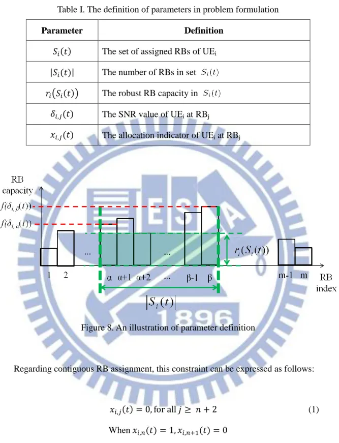
By expressing as ILP problem, the objective of our proposed algorithm is to maximize the LTE UL system throughput, while keeping the constraint at the same time. Before starting formulate problem, we first introduce some parameters listed in Table I. We first define as the set of assigned RBs of and represents the number of RBs in set . Also, let and be the channel signal-to-noise ratio (SNR) measured by UEi at RBj and the robust RB capacity at RBs that UEi operate, respectively. Besides, is

14

an allocation indicator of UEi at RBj. If RBj is allocated to UEi by scheduler, is assigned to 1. Otherwise, is assigned to 0. An illustration of these parameters is shown in Fig.8. In this example, can be expressed as

Hence, which counts the number in can be derived as

From , we know the scheduler allocates RBs to UEi. Consequently, the allocation indicator of UEi at all the RBs can be assigned as follows:

The particular is the rectangle height of UEi at RBj, in which the f() is an mapping function which can get the maximum available data rate of a specific through looking up the MCS table. Thus, and are the height of UEi at and , respectively. Finally, having above information, we can get as

15

Table I. The definition of parameters in problem formulation

Parameter Definition

The set of assigned RBs of UEi The number of RBs in set

The robust RB capacity in

The SNR value of UEi at RBj

The allocation indicator of UEi at RBj

Figure 8. An illustration of parameter definition

Regarding contiguous RB assignment, this constraint can be expressed as follows:

(1) When

The equation (1) descripts that as is allocated to while is not, the RBs from to cannot be able to anymore. Thus, this equation ensures the constraint of contiguous RB assignment.

16

In spite of the contiguous RB assignment constraint, the other inherent constraint, robust MCS mode, should also be followed. Since UE has different channel quality among RBs, the maximum available data rate and corresponding MCS can hence be different. For this reason, the height is introduced, which represents the least RB capacity among all allocated RBs of . As the specification defined, the active UEs report the instantaneous UL channel quality, as known as SNR value , through SRS coding sequences on each RBj to the serving eNodeB, periodically. The eNodeB maps the SNR value to achievable MCS mode on all RE within each RB, and then RB capacity of each RB is determined. The approach is proposed in [23]. The height _{of a RB rectangle can be expressed as} follows:

(2)

where f() function as mentioned before is to derive the maximum available RB capacity from specific channel SNR value . In general, f function can be implemented by a look-up table in eNodeB as shown in Table II. The RB capacity can be calculated by equation (3) [24].

(3)

where nbits/symbol computes how many bits carried per symbol, as the same as per RE, and it can be retrieved directly by which MCS mode is employed. nsymbols/slot is the number of symbols per slot, nslot/TTI is the number of slots per TTI and nsc/RB is the number of sub-carriers per RB. Table II shows the mapping table in which the MCS mode begins from QPSK (1/2) to 64QAM (3/4). In this table, must be larger than or equal to the SNR threshold, so the corresponding MCS mode can be applied. For example, one at

17

having 8 means this RB can be modulated as QPSK (1/2), QPSK (2/3), QPSK (3/4) or 16QAM (1/2), but cannot be modulated as 16QAM (2/3) and the rest MCS.

Table II. The mapping table from SNR threshold to MCS

MCS mode SNR threshold (dB) nbits/RE RB capacity (Kbps)

QPSK(1/2) 1.7 1 168 QPSK(2/3) 3.7 1.33 224 QPSK(3/4) 4.5 1.5 252 16QAM(1/2) 7.2 2 336 16QAM(2/3) 9.5 2.66 448 16QAM(3/4) 10.7 3 504 64QAM(2/3) 14.8 4 672 64QAM(3/4) 16.1 4.5 756

In addition to the constraints of contiguous RB assignment and robust MCS mode formulated at equation (1), (2) and (3). There still exist some inherent constraints because of our system model assumption. Equation (4) is expressed as follows:

(4)

Since the MIMO is not taken into consideration, this equation illustrates that each RBj can be assigned to at most one UE. Moreover, of each UEi is counted through:

18

To ensure the total allocated RBs at a specific TTI t doesn’t exceed the supported UL bandwidth, we used the following equation to limit the number of allocated RBs:

(6)

Finally, we assume the scheduler performs resource allocation per TTI t. Therefore, the system throughput maximization problem can be well-formulated by equation (7):

(7)

Subject to the constraints of (1)(2)(3)(4)(5)(6)

3.3 Heuristic Method

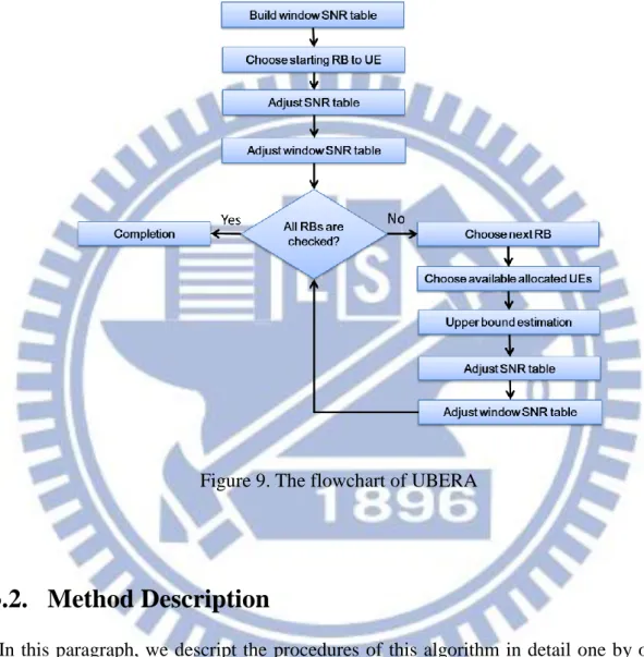
Since the problem of LTE UL scheduling described as above has been proven to be NP-hard [25]. Thus it is not possible to achieve the maximal system throughput performance in polynomial time. To compromise with the complexity, we present a heuristic algorithm: Upper Bound Estimation Resource Allocation (UBERA).

Before starting, some additional parameters are introduced to help describe our algorithm. As to the system model described, we assume there are m RBs and n UEs in the cellular network at TTI t. Let M and M’ be the sets of non-checked and checked RBs, respectively.

Also, let N and N’ be the sets of available scheduled and non-available scheduled UEs,

respectively. Initially M={RB1, RB2, …, RBm}, and N={UE1, UE2, …, UEn,}; M’ and N’ are

both . For simplicity, we use |●| to indicate the number of elements in a set. For example, initially |M| = m and |N| = n. Besides, , where N, M, represents the measured SNR value of UEi in RBj.

19

3.3.1. Brief Introduction

The main characteristic of UBERA is that as each time it tries to allocate one RB to UE, the algorithm gets all available allocated UEs on the RB, and calculates the upper bound after allocating to the UEs, respectively. After getting all upper bound values of different UEs, UBERA gives the RB to the UE which has the maximal upper bound. The reason of adopting this method is that the common existing scheduling algorithms for LTE UL allocate the RB to the UE, which has the highest SNR at the RB or can derive the current maximal sum system throughput, but doesn’t consider the future influence after this allocation. Thus, it is possible that the allocation can temporarily increase system throughout, but may become worse in the latter scheduling due to robust MCS mode.

The flowchart of UBERA is illustrated in Fig.9. Firstly, the algorithm calls “Build window SNR table.” In this procedure, we take SNR table, which records all the active UEs to RBs channel conditions, as reference to build a brand-new table called window SNR table. After the table is built, this goes to “Choose starting RB to UE” procedure, which decides the first RB to be checked. Besides, the checked RB is also allocated to one active UE here. To keep the constraint of robust MCS mode, we hence call “Adjust SNR table” which adjusts the values recorded in SNR table. Since the window SNR table is built based on SNR table, the “Adjust window SNR table” is called to adjust the values recorded in window SNR table. Before start allocating next RB to UE, we check whether there are available RBs unchecked. If all the available RBs in system are checked, the algorithm is terminated here. In case that there is RB unchecked, the algorithm in “Choose nest RB” procedure chooses one RB from unchecked RBs. Since the later “Upper bound estimation” is the core of this algorithm, which consumes most of the time, taking all the UEs to this procedure to implement estimation will waste too much time. Thus, we call “Choose available allocated UEs” to choose some candidate UEs. In “Upper bound estimation,” the upper bounds of candidate UEs are

20

calculated and the chosen RB is allocated to the candidate UE whom has the maximal upper bound. The “Adjust SNR table” and “Adjust window SNR table” are called to follow robust MCS mode. Finally, this algorithm backs to check whether there RBs unchecked.

Figure 9. The flowchart of UBERA

3.3.2. Method Description

In this paragraph, we descript the procedures of this algorithm in detail one by one. The procedures are described follows.

(1) Build window SNR table

Before start scheduling, the algorithm first defines a term called window. Here, we denote it as w. Besides, the w has a size called window size, which is an odd number less than or equal to m and denotes it as ws. The w is a rectangle that can once cover several RBs based on

21

minimum SNR in the w is selected as window SNR, and put the value on the RB1 of UE1 in

window table. Here, the window SNR of UEi at RBj as wSNRi,j is expressed as:

We then slide the window to RB2 of UE1, and get wSNR1,2. After the w has put on every RBs of each UE, we finally completely build window table with values from wSNR1,1, wSNR1,2,

wSNR1,3,…, wSNR1,m, wSNR2,1,… to wSNRn,m. The reason of building the window table is that

the LTE UL must keep to contiguous RB assignment and robust MCS mode. Hence, the minimum SNR in w can be taken as the possible average SNR after allocating the RB, which we predict in prior.

(2) Choose starting RB to UE

For each , it first calculates the difference between maximal and second maximal

wSNRi,j, which is denoted as .The of a specific is expressed as:

where and is the maximal and second maximal at . It then picks , which has the maximal , and allocates to UE whom owns at . However, if there are more than one having same maximal difference, the scheduler then picks the , which has the maximal among these same maximal , and allocates to the UE whom owns this . Then, the procedure removes the just allocated from M to M’.

(3) Adjust SNR table

22

UEi. After getting one from previous procedure (“Choose starting RB to UE” or “Upper bound estimation”), where is just allocated to , the sub-program checks all the of UEi, which denotes as . If is larger than and not equals to , the

is revised to .

(4) Adjust window SNR table

In this sub-program, it revises the window table, which is first built at “Build window SNR table.” Here, we check the UEs in N one by one. At first, it puts w on the first left side

non-allocated RB of allocated RBs of UE in N. Then, if the most left side allocated RB is not

the current UE getting from N, the wSNRi,j is revised as

We then slide w to the second left side non-allocated RB, and revise the wSNRi,j as

.

The w continually slides left and revises wSNRi,j. Until the wSNRi,j is revised as

the UE stops. However, if the UE in N equals to the UE of most left side allocated RB, it first

towards right looking for the most right allocated RB of this UE, and denotes the RB as .

Then, the w is similarly puts on the first left side non-allocated RB, . If , it stops, else the wSNRi,j is revised as

23

Then we slide w left, and revise the wSNRi,j as

until , it stops. After the wSNRi,j at left side non-allocated RBs of UEs

in N is totally adjusted, the procedure tries to revise the wSNRi,j at right side non-allocated

RBs of allocated RBs, which is similar to the description described above. At first, it puts w on the first right side non-allocated RB of allocated RBs of UE in N. If the most right side

allocated RB is not the current UE getting from N, the wSNRi,j is revised as

We then slide w to the second right side non-allocated RB, and revise the wSNRi,j as

The w continually slides right and revises wSNRi,j. Until the wSNRi,j is revised as

24

first towards left looking for the most left allocated RB of this UE, and denotes the RB as . Then, the w is similarly puts on the first right side non-allocated RB, .If

, it stops,else the wSNRi,j is revised as

Then we slide w right, and revise the wSNRi,j as

until , it stops. (5) Choose next RB

At this procedure, the scheduler tries to determine the next RB from M to allocate. Let the

first un-allocated RB on the left side of allocated RBs be , and the first un-allocated RB on the right side of allocated RBs be . The decision value of is , where allocates to . Besides, the decision value of is ,

where allocates to . However, if allocates to virtual UE (the term

here means not allocated to any real UE), the decision value of will be the maximal among all the s, where N and available to be scheduled at . Similarly, if allocates to virtual UE, the decision value of will be the maximal among all the s, where N and available to be scheduled at . The scheduler then picks as next RB to allocate if the decision value of is larger than or equal to the decision value of , else picks However, if there is no , it returns directly, and returns if there is no . Finally, if

25

there is no remaining RB to schedule, the algorithm terminates at here. (6) Choose available allocated UEs

After picking RB (denotes as , where M) from “Choose next RB”, the scheduler determines the available UEs at here. If the side of , which is allocated before (denotes as , where M’), is to virtual UE, it goes to “Upper bound estimation” directly (1). However, If is not to virtual UE and there are some UEs’ , where N and available to be scheduled at (denotes as ), is larger than or equal to , where allocates to , it then picks all these larger valued UEs with to “Upper bound estimation” (2). On the contrary, if of all is less than , it checks as follows. First, it gets all the UEs of , which has the maximal at among all the RBs of the UE, where RBs M and calculates the gain as follows:

,

where is the second maximal among all the RBs M of the UE. Here, the first term of the formula means the gain after allocating to , and the second term means the gain after allocating to , respectively. If there exists UEs whose , which means allocating to may cause the gain of the UEs down, then the scheduler picks all UEs whose with to “Upper bound estimation” (3). However, as all the UEs’ or no have maximal at , and this allocation can promote the system throughput, it allocates to , removes from M to M’; else it goes to “Upper bound estimation” (4).

(7) Upper bound estimation

At this procedure, the scheduler calculates the upper bound after allocating to available UEs, which determines at “Choose available allocated UEs”, respectively, and

26

allocates to the UE whom has maximal upper bound. In (1) and (4) of “Choose available allocated UEs”, the available UEs are . The available UEs of (2) and (3) are picked at “Choose available allocated UEs”. Here, let the UEs available to be pseudo-allocated at left side of allocated RBs be , which belongs to N and not

includes the UE, whom obtains the most right side allocated RBs, if the UE is blocked at left side by another UE. Besides, let the UEs available to be pseudo-allocated at right side of allocated RBs be , which belongs to N and not includes the UE, whom obtains the

most left side allocated RBs, if the UE is blocked at right side by another UE. The upper bound of a specific UEi is predicted as follows.

At first, the scheduler pseudo-allocates to UEi, and calculates the temporal upper

bound. If UEi not equals to , whom obtains , the thus cannot be used at

current prediction, since it has been blocked by UEi. The scheduler here kicks from

, if is at left side of allocated RBs; else kicks from . Second, it sorts RBs M, which doesn’t include based on maximal , where for left side non-allocated RBs or for right side non-allocated RBs. After sorting, it picks the highest priority RB and calculates the temporal upper bound after pseudo-allocating to or depends on the place of the RB, respectively. Since all the temporal upper bounds of pseudo-allocating the highest priority RB to different or have been completed, the scheduler chooses the maximal bound of this pseudo-allocating. It then picks the second highest priority RB and does the same thing, and stops until all the RBs in sorting results have been picked. After all prediction is completed, each UE available to be allocated at has upper bound estimation. The scheduler then real allocates to the UE, whom has maximal upper bound among available UEs. Finally, it removes from M to M’, and if this allocation cause the UE, whom obtains , blocked, then removes the UE from N to N’.

27

3.3.3. Detailed Example

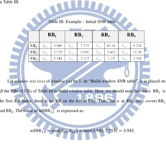
A detailed example is illustrated in this paragraph, in which we assume the UL bandwidth is divided into 4 RBs (denoted as , , and ) and 3 active UEs (denoted as , and ) want to transmit UL resources. After active UEs reporting their channel qualities to eNodeB, the eNodeB gets SNR values of active UEs as shown in Table III.

Table III. Example – Initial SNR table

Let window size (ws) of window (w) be 3. At “Build window SNR table”, w is placed on all the RBs of UEs of Table III to build window table. Here, we should note that since is the first RB index, there is no RB on the left of . Thus, the w at only covers and . The value of is expressed as:

Similarly, since is the last index, there is no RB on the right of . Thus, the w at only covers and . The value of is expressed as:

28

For and , there is RB both on left and right. The w can hence properly cavers , and for . For , the w can properly covers , and . The value of and are expressed as:

The procedure of deriving values of and from SNR values is similar to . The result is shown in Table IV

Table IV. Example – Build window SNR table

At “Choose starting RB to UE”, we first calculate , , and , respectively. For , and . Thus, can be calculated as:

For , and . Thus, can be calculated as:

29

For , and . Thus, can be calculated as:

The calculation of is similar to , and , which is 0.769. Since is the maximal, is chosen as starting RB at this procedure. Besides, belongs to , we hence allocates to . The result is shown in Table V, where the red grid on of manes the allocated to .

Table V. Example – Choose starting RB to UE

Since the latest scheduling allocates to , is get at “Adjust SNR table”. In this procedure, SNR values of are checked. If the checked SNR value is larger than , the SNR value is assigned to value of . From observation, we know value of , and is less than . Thus, the SNR value doesn’t need to revise. The result is shown in Table VI, where the red bold word 10.66 is .

30

Table VI. Example – Adjust SNR table

At “Adjust window SNR table”, is first on the left side of allocated RBs. Since the right side of is allocated to and , doesn’t need to revise left side unchecked RBs. For , new is calculated as:

Since the new equals to original one, doesn’t need to revise. Besides, the stop determination happens at , we don’t need to check and . For , new is calculated as:

Since the new not equals to original one, which is 1.23, is adjusted to 2.113. Similarly, the stop determination happens at , we don’t need to check and . For right side unchecked RBs, is first on the right side of allocated RBs. Since the left side of is allocated to and , doesn’t need to revise right side unchecked RBs. For , new is calculated as:

31

Since the new not equals to original one, which is 7.462, is adjusted to 10.58. The procedure of is similar to , and is adjusted to 3.701. The result of this procedure shows in Table VII, in which the red bold words are revised values.

Table VII. Example – Adjust window SNR table

At “Choose next RB” procedure, is and is . Due to the right side of is , which is allocated to , the decision value of is . On the other hand, the left side of is also , the decision value of is . Since , is chosen as . The result is shown in Table VIII, where the yellow grid on means is chosen to be checked.

32

At “Choose available allocated UEs”, is not allocated to virtual UE. Thus the condition (1) of this procedure is skipped. Since is larger than , condition (2) is met, where . The result shows in Table IX, where the yellow grids on of and of means and are selected in set.

Table IX. Example – Choose available allocated UEs

At “Upper bound estimation”, for , and . Since the decision value of , which is , is larger than , which is , the sorting list of is .At first, is pseudo-allocated to , and gets 16.462. Then the upper bounds after pseudo-allocating to , or are 23.259, 22.068, 18.575 and 16.462, respectively. Since the upper bound after pseudo-allocating to is maximal, is pseudo-allocated to and gets 23.259. Similarly, for , the upper bounds after pseudo-allocating to , or are 15.78, 25.838, 25.8 and 23.259, respectively. Since 25.838 is maximal and no RBs need to calculate, the upper bound estimation of allocating to is 25.838. The calculations of allocating to or are similar to above, in which the estimation of is 28.627. Besides, the estimation of is 18.807. Due to the upper bound estimation of is larger than and , which is 28.627, thus we allocates to . The result shows in Table X, where the green grid on of manes obtains .

33

Table X. Example – Upper bound estimation

The rest of this example follows the flowchart in Fig. 9. The scheduling result is shown in Table XI, where is allocated to , are allocated to , and is allocated to .

Table XI. Example – Scheduling result

3.3.4. Pseudo Code and Time Complexity

To help analysis time complexity of proposed algorithm – UBERA, we present the pseudo codes here. In Table XII., we list the main body. Besides, Table XIII and Table XIV list the “Adjust SNR table” and “Adjust window SNR table” procedure, respectively.

In Table XII, line 1 to line 16 execute “Build window SNR table”, which build a brand-new table based on SNR values, where eNodeB get from UEs’ periodically report. Here, the SNRs in window size of UE at specific RB are all checked at line 8, and find the minimum among these SNRs as corresponding wSNR at line 9. From line 18 to line 35,

34

“Choose starting RB to UE” is executed, where we get all the ∆j from line 24 to line 29. At line 30, we check whether there are ∆js having same value as max∆j. The RB decision and allocation is from line 31 to line 35. At line 37, “Adjust SNR table” is executed and listed in Table XIII. In Table XIII, SNR of RB of specific UE is got at line 5, checked at line 6 and assigned at line 7. At line 38 of Table XII, “Adjust window SNR table” is executed and listed in Table XIV. In Table XIV, the searching order of RBs, which are in window size of left side non-checked RBs, is decided at line 7 and line 8. The searching order of RBs, which are in window size of right side non-checked RBs, is decided at line 9 and line 10. Besides, the new wSNR is continued updated from line 12 to line 19, and revise the old wSNR at line 21.

At line 40, algorithm goes into while-loop for allocating remaining non-checked RBs. From line 42 to line 70, “Choose next RB” is executed to pick one of non-checked RBs. If no RB needs to check, we return “no remaining RB needs to be checked” at line 47. The decision value of and got from line 55 to line 59 and from line 60 to line 64, respectively. From line 65 to line 69, RB to be checked is chosen. If “no remaining RB needs to be checked” is returned, the algorithm is terminated at line 73. Otherwise, “Choose available allocated UEs” is executed to choose candidate UEs from line 76 to line 83. From line 85 to line 100, “Upper bound estimation” is executed, in which the upper bound value of UE is calculated at line 93 according to 3.3.2 (7), and the decision of is from line 94 to line 97. In line 102, “Adjust SNR table” is executed to Table XIII. Besides. “Adjust window SNR table” is also executed to Table XIV.

Table XII. Pseudo code of UBERA

1: // Build window SNR table 2: Let ws be the size of the window 3: Let be the minimum SNR in ws 4: for each UE i in the system do

35 5: for each RB j in the system do

6: ← infinitely large;

7: for each RB c in the ws of j do

8: Let be the SNR of UE i on RB c

9: if (c is in the legal range of RB) and ( is less than ) then

10: ← ;

11: end if 12: end for

13: Let be the window SNR of UE i on RB j

14: ← ;

15: end for 16: end for 17:

18: // Choose starting RB to UE

19: Let be the 1st high window SNR on RB j, which belongs to UE i 20: Let be the 2nd high window SNR on RB j, which belongs to UE i’ 21: Let ∆j be the difference between and at RB j

22: Let max∆j be the maximum of all the ∆j 23: max∆j ← -1;

24: for each RB j in the system do 25: ∆j ← ; 26: if ∆j is larger than max∆j then 27: max∆j ← ∆j;

28: end if 29: end for

30: Check if other RB j’ has the same ∆j’ as max∆j, where j’ is not equal to j 31: if doesn’t have then

32: Allocate RB j of max∆j to UE i 33: else

34: Allocate RB j to UE i, who has the same ∆j as max∆j and is the maximum

35: end if 36:

37: Execute Adjust SNR table [Table V.];

38: Execute Adjust window SNR table [Table VI.]; 39:

40: while (true) do 41:

36

43: Let be the first un-checked RB index on the left side of already checked RBs

44: Let be the first un-checked RB index on the right side of already checked RBs

45: Let be the chosen RB here

46: if both and doesn’t exists then 47: no remaining RB needs to be checked 48: else if doesn’t exist then

49:

50: else if doesn’t exist then 51:

52: else

53: Let be the decision value of 54: Let be the decision value of 55: if right side of is allocated to virtual UE then

56: ← maximum window SNR of UEs, who is allowed to be allocated at

57: else

58: ←window SNR of UE at , who is already allocated at right side of

59: end if

60: if left side of is allocated to virtual UE then

61: ← maximum window SNR of UEs, who is allowed to be allocated at

62: else

63: ←window SNR of UE at , who is already allocated at left side of

64: end if

65: if is larger than then 66: 67: else 68: 69: end if 70: end if 71:

72: if no remaining RB needs to be checked then 73: break;

74: end if 75:

37 77: Let c be

78: Let be the window SNR of UE u at c, which is already allocated at the side of c 79: if (u is real UE) and (there exists other UE allowed to be allocated at c, and has higher

window SNR than ) then

80: Let I be the set of UEs allowed to be allocated at c, whom has higher window SNR than

81: else if (u is virtual UE) or ((u is real UE) and (allocate c to u will cause the total system throughput down)) then

82: Let I be the set of UEs allowed to be allocated at c

83: end if 84:

85: // Upper bound estimation 86: if I is empty then

87: allocate c to u 88: else

89: Let be the upper bound value of UE i

90: Let be the maximum among all the s, which belong to UE 91: = -1;

92: for each UE i in I do

93: Calculate according to 3.3.2(7) 94: if is larger than then

95: ← 96: ← ; 97: end if 98: end for 99: allocate c to 100: end if 101:

102: Execute Adjust SNR table [Table V.];

103: Execute Adjust window SNR table [Table VI.]; 104: end while

Table XIII. Pseudo code of Adjust SNR table

1: Let c be the latest scheduled RB, which is allocated to UE i 2: if UE i is not a virtual UE then

38 4: for each RB j in the system except c do

5: Let be the SNR of UE i on RB j 6: if is larger than then 7: ← ;

8: end if 9: end for 10: end if

Table XIV. Pseudo code of Adjust window SNR table

1: Let i’ be the latest allocated UE 2: Let ws be the size of the window 3: Let be the minimum SNR in ws

4: for each UE i in the system do 5: for each RB j in the system do 6: = infinitely large;

7: if (j is not allocated) and (is at left side of allocated RBs) then 8: check RB c form low to high index at 12:

9: else if (j is not allocated) and (is at right side of allocated RBs) then 10: check RB c from high to low index at 12:

11: end if

12: for each RB c in the ws of j do

13: Let be the SNR of UE i on RB c

14: if (((i is not i’) and (c is not allocated to any UE)) or ((i is i’) and (c is not allocated to any UE or allocated to i’))) and (c is in the legal range of RB) and ( is less than ) then

15: ← ;

16: else if ((i is not i’) and (c is allocated to UE)) or ((i is i’) and (c is allocated to UE but not i’)) 17: break;

18: end if 19: end for

20: Let be the window SNR of UE i on RB j

21: ←

22: end for 23: end for

39

At “Build window SNR table”, it checks all RBs of all UEs to build the window table. Since the size of w is ws, it takes . At “Choose starting RB to UE”, the scheduler first checks all RBs of UEs to get and of all RBs, and calculates . Thus it takes . Finding maximal , checking same maximal , and allocating to UE only needs to check all the . It here takes . Thus, the complexity at “Choose starting RB to UE” takes . Besides, “Adjusts SNR table” revises all of a specific UEi, thus it takes scanning all the RBs. Let the number of

RBs be checked currently as c. “Adjust window SNR table” revises window table similar to “Build window SNR table”, but doesn’t revises the checked RBs. Hence, the scheduler takes . Since and are updated after each allocation, it doesn’t take any time to find the two RBs. The worst case of “Choose next RB” is that and both are allocated to virtual UE. Thus, it takes to find the decision values of and from N. In the worst case of “Choose available

allocated UEs”, all the UEs have the maximal at among all the RBs of the corresponding UE. Thus, it takes to find the second maximal and calculates . At “Upper bound estimation”, the worst case is that all the UEs belong to , and . It hence takes . The outside means the number of . is the number of unallocated RBs, which needs to predict but doesn’t include , since is pseudo-allocated at outside . The inside is the number of or . Finally, the inside is used to pseudo-adjust , which is similar to “Adjust SNR table” and calculates the corresponding upper bound after pseudo-allocating to or . So the total time complexity of the proposed method can be calculated as

40

Since “Adjust SNR table” and “Adjust window SNR table” are called after each resource allocation, these two procedures run m times, respectively. Besides, since the first RB is allocated at “Choose starting RB to UE”, the “Choose next RB”, “Choose available allocated UEs” and “Upper bound estimation” run (m-1) times.