Investigation of long-term transport in Tanshui River estuary, Taiwan

JOURNAL OF WATERWAY, PORT, COASTAL, AND OCEAN ENGINEERING / MARCH/APRIL 2001 / 61

I

NVESTIGATION OF

L

ONG

-T

ERM

T

RANSPORT

IN

T

ANSHUI

R

IVER

E

STUARY

, T

AIWAN

By Wen-Cheng Liu,

Ming-Hsi Hsu,

and Albert Y. Kuo,

Member, ASCE

ABSTRACT: The net, long-term transport of materials in estuaries is governed primarily by the residual (or tidally averaged) circulation in the system. Knowledge of the residual circulation is essential for predicting the transport of algal patches, debris, and pollutants of concern in an estuary. A real-time, two-dimensional, laterally averaged hydrodynamic model is used to analyze residual current and salinity distributions in the Tanshui River estuary. The model results were filtered to arrive at the subtidal, or residual quantities. The characteristic two-layered estuarine circulation prevails for most of the time at Kuan-Du station near the river mouth. Though the circulation strengthens with increasing river discharge at low flow, its strength decreases at moderate river discharge and the two-layered circulation ceases at moderately high flow. This implies a weak trapping capacity in the estuary. At the upriver stations where salinity is lower, strength of circulation generally decreases with increasing river discharge. The response of residual velocity to the spring-neap cycle indicates stronger residual circulation during neap tide than spring tide.

INTRODUCTION

The estuary is the primary conduit for the transport of water and materials from its drainage basin to the coastal ocean. The ultimate fates of land-derived materials, such as pollutants, de-pend on the water movement in the estuaries. In addition to the ebb and flood of tidal flow, net estuarine circulations are also forced by freshwater runoff, by seawater intrusion, by the nonlinear interactions of the tidal current with shoreline con-figuration and bathymetry, and occasionally by the meteoro-logical forcing. The long-term, large-scale transport and dis-tribution of waterborne materials such as salt, sediment, and pollutants are primarily determined by these residual net cir-culations, though the tidal flow contributes to the dispersion process. The discharge of runoff from the drainage basin dic-tates a net movement of water toward the ocean. However, the intrusion of seawater from the ocean often results in a net estuarine circulation of upriver flow in the lower layer and downriver flow in the upper layer of the water column (Prit-chard 1956). It is this net estuarine circulation that dominates the long-term transport of material in coastal plain estuaries.

In a narrow and relatively straight estuary, the net estuarine circulation, or residual current, is forced by the balance of the average surface slope and density gradient (primarily by the salinity gradient). It is controlled by the complicated interac-tion of river discharge, tide, and estuarine geometry. Hansen and Rattray (1965) proposed a theoretical model of the estu-arine circulation that depends on the relative magnitudes of river flow, density gradient, tidal mixing, and river geometry. This model is a powerful diagnostic tool, providing a frame-work for evaluating the response of estuarine circulation and salinity structure to various forcing mechanisms. However, it is not a predictive tool because it does not elucidate the inter-relationship among the forcing mechanisms. In the case of a simple homogeneous flow with no salinity gradient nor river discharge, Ianniello (1977) showed that the mean Lagrangian transport in a tidal channel has a two-layered flow pattern. The

1

Sr. Res. Engr., Hydrotech Res. Inst., Nat. Taiwan Univ., Taipei 10617, Taiwan.

2

Prof., Dept. of Agric. Engrg., and Sr. Res. Fellow, Hydrotech Res. Inst., Nat. Taiwan Univ., Taipei 10617, Taiwan.

3_{Prof., School of Marine Sci./Virginia Inst. of Marine Sci., Coll. of} William and Mary, Gloucester Point, VA 23062.

Note. Discussion open until September 1, 2001. To extend the closing date one month, a written request must be filed with the ASCE Manager of Journals. The manuscript for this paper was submitted for review and possible publication on December 28, 1999; revised August 8, 2000. This paper is part of the Journal of Waterway, Port, Coastal, and Ocean

Engineering, Vol. 127, No. 2, March/April, 2001.䉷ASCE, ISSN

0733-950X/01/0002-0061–0071/$8.00⫹ $.50 per page. Paper No. 22150.

surface layer flows are directed landward and the bottom layer flows are directed seaward. However, this tidally induced cir-culation may be easily masked by the density induced current in estuaries with freshwater inflow and a small tidal amplitude to depth ratio (Ianniello 1981). Park and Kuo (1996a) used theoretical analyses to demonstrate various feedback loops among the forcing mechanisms of estuarine circulation. They further employed a numerical model to investigate the result-ing effect of competitive mechanisms in a partially mixed es-tuary. In the general case of estuaries with river discharge and salinity gradient, interaction among the forcing mechanisms and geometry is so complicated that a numerical model has to be resorted to for prediction of residual circulation.

A number of numerical models have been applied to sim-ulate and study the hydrodynamic behaviors of various estu-aries in various parts of the world. However, the investigation of the tidal dynamics and estuarine circulation in the Tanshui River system of Taiwan is rather limited. Hsu (1969) made a rudimentary analysis of the tidal current in the lowest reach of the estuary. Ouyang (1971) used a one-dimensional tidally averaged model to study pollutant transport and dissolved ox-ygen distribution in the system. The transports by tidal current and residual circulation were lumped into a single dispersion term in the model. Yen and Hsu (1982) applied a one-dimen-sional real-time model to the Tanshui River system. Hsu (1998) further used a horizontal two-dimensional model to in-vestigate the influence on hydrodynamics by the proposed flood protection structures at Kuan-Du plain and Sheh-Tse is-land. Both model applications emphasized flood routing, and no analysis of tide nor long-term circulation was attempted. A harmonic analysis of tide was conducted for two stations in the lower part of the estuary (Water Resource Planning Com-mission 1989). Amplitudes and phases of principal tidal con-stituents were obtained. Chang and Shi (1989) made a descrip-tive analysis of the tidal propagation in the Keelung River, one of the three branches of the Tanshui River system. Since then, several modeling studies were conducted for the Keelung River, in conjunction with either the river training or the sew-age interception project. Hsu et al. (1999) applied a laterally averaged two-dimensional model to the Tanshui River. They treated the estuarine system, including the main stem and trib-utaries, as a whole and made the first systematic analysis of its hydrodynamic behaviors. Both their model results and data analysis confirmed that two-layered estuarine circulation exists in the system. This paper further analyzes the results of model simulations to investigate the long-term transport processes in the system. The model results were filtered to arrive at the subtidal or tidally averaged quantities. The characteristics of estuarine circulation (residual current) and their implication to

62 / JOURNAL OF WATERWAY, PORT, COASTAL, AND OCEAN ENGINEERING / MARCH/APRIL 2001 FIG. 1. Map of Tanshui River Estuary

long-term transport were investigated. Its variability in re-sponse to forcing mechanisms was also examined.

ESTUARY AND NUMERICAL MODEL

The Tanshui River is formed by the confluence of Tahan Stream, Hsintien Stream, and Keelung River (Fig. 1). The es-tuarine reach is more than 20 km in length, and the average river width and depth are about 600 m and 6.5 m, respectively. The downstream portions of all three tributaries are influenced by the tide, and subjected to seawater intrusion. Together, they form the largest estuarine system in Taiwan, with its drainage basin including the capital city of Taipei. Its drainage area encompasses 2,728 km2

, with a total channel length of 327.6 km. The major portion of the estuary system, upstream of Kuan-Du (Fig. 1), lies within the Taipei basin, while the stretch downstream is confined by high mountains on both sides. Because of the presence of mountains and narrows of the river, there are no significant wind-induced currents in the river. Except for the occasional storm surges induced by hur-ricanes, the major forcing mechanisms of the barotropic flows are the astronomical tide at the river mouth and river dis-charges at upriver ends. Semidiurnal tides are the principal tidal constituents, with a mean tidal range of 2.22 m and a spring tidal range of 3.1 m. The average river discharges are 62.1 m3

/s, 72.7 m3

/s, and 26.1 m3

/s, respectively, in the Tahan Stream, Hsintien Stream, and Keelung River. In addition to the barotropic flows forced by the tide and river discharges, the baroclinic flow forced by seawater intrusion is another im-portant transport mechanism in the Tanshui River estuary sys-tem.

A laterally averaged two-dimensional model was applied to the Tanshui River estuary system (Hsu et al. 1999). The orig-inal version of the model was developed by Park and Kuo (1993), and has been applied successfully to the tributary es-tuaries of the Chesapeake Bay in the United States (Park and Kuo 1994, 1996b). The model solves the continuity, momen-tum, and mass-balance equations by a two-time level,

finite-difference scheme with a spatially staggered grid. The implicit treatment of the vertical diffusion terms results in a tridiagonal matrix in the vertical direction. The QUICKEST scheme is used to express the finite-difference form of the advective term. It is based on a conservative control volume formation and estimates the cell wall concentration with a quadratic in-terpolation using concentrations in two adjacent cells and that in the next upstream cell. The method of the solution is de-tailed in Park and Kuo (1993). The model includes a frame-work for coupling the shoals and shallow embayments with the main channel (Kuo and Park 1995). They demonstrated that the accounting of mass and momentum exchanges be-tween the main channel and shallow areas is essential not only for the computation of the conditions in the shallow areas, but also for proper simulation of tidal propagation along the main channel. If the water and momentum exchanges between the shallow areas and the main channel are not accounted for, a model cannot reproduce the along-channel variations of both the tidal range and the tidal phase. This coupling framework proposed was refined and adopted to fit the model for the Tanshui River system.

The model was also expanded to include the capability to simulate tributaries as well as the main stem of estuaries (Hsu et al. 1996, 1997, 1999). In applying it to the Tanshui River system, the model treats the Tanshui River and Tahan Stream as the main stem, and the Hsintien Stream and Keelung River as tributaries. The model is supplied with data describing the geometry of the Tanshui River system. The geometry in the vertical 2D model is represented by the width at each layer at the center of each grid well. A field survey in 1994 done by the Taiwan Water Conservancy Agency collected the cross-sectional profiles at about 0.5 km intervals along the tidal por-tion of the river. These profiles were used to schematize the river system. The three branches are divided into 33, 14, and 37 segments, respectively, with a uniform segment length of 1.0 km. The vertical layer thickness is 1 m for all layers except for the surface layer, which is variable, with 2 m at mean sea level. The maximum number of layers is 10 at the deepest

JOURNAL OF WATERWAY, PORT, COASTAL, AND OCEAN ENGINEERING / MARCH/APRIL 2001 / 63

FIG. 2. Longitudinal Bottom Profile of Tanshui River–Tahan Stream

section of the river. Fig. 2 shows the bottom profiles of the schematized cross section and the deepest point of the mea-sured section along the Tanshui River – Tahan Stream. Details of model calibration and verification have been presented in Hsu et al. (1996, 1997, 1999). In the following, a brief de-scription is presented.

Manning’s friction coefficient and the coefficients for tur-bulent mixing terms are important calibration parameters af-fecting the calculation of surface elevation, current velocity, and salinity distribution. The preliminary calibration of Man-ning’s friction coefficient used a single constituent tide, M2, to

reproduce the longitudinal distribution of the mean tidal range. The results show that the average absolute value of the dif-ferences (mean absolute errors) between computed and mea-sured tidal ranges is 3.4 cm, while the root-mean-square error is 3.8 cm, both of which are less than 2% of the mean tidal range. The fine-tuned calibration compares the along-river var-iations of amplitude and phase of the individual constituents, using a nine-constituent tide to force the system at the river mouth. The results also compare times of high tide and low tide between computation and observation. The difference be-tween the model results and the observations is less than 10 min. The calibrated model has a Manning’s friction coefficient ranging from 0.032 to 0.026 in the Tanshui River – Tahan Stream, 0.015 for the Hsintien Stream, and from 0.023 to 0.016 for the Keelung River.

The calibration of mixing processes and verification of the flow field were conducted through model simulation of pro-totype conditions during the period of March 15 to September 30, 1994. The model was driven by three time-varying bound-ary conditions — measured daily freshwater inflow through the upstream boundaries, hourly tidal elevation, and linearly in-terpolated salinity from measured data at the river mouth. The mixing processes are modeled with turbulent diffusion terms. The mixing length concept is used to calculate the eddy vis-cosity and diffusion coefficient in the vertical direction. The formulations similar to those proposed by Pritchard (1960) are used in the model. The tidal average salinity and time series data measured on April 12 and June 24, 1994 were used to

calibrate the constants in the formulation of the vertical dif-fusion coefficient. The results show that the mean absolute errors and root-mean-square errors of the difference between the computed and hourly measured data are from 0.13 to 1.76 parts per thousand (ppt) and from 0.16 to 2.45 ppt, respec-tively, at various stations. The computed water surface eleva-tions and current velocities were compared with time series data at various stations to verify the barotropic flow compo-nent. The measured and computed longitudinal velocities at selected stations were averaged over the tidal cycle. The ver-tical profiles of the measured and computed residual velocities were compared, and verified with analytical models of Hansen and Rattray (1965). The results have been reported by Hsu et al. (1999).

The model’s ability to predict mass transport was verified with a simulation of salinity distribution from March 15 to April 30, 1995. The model predictions agree well with the field measurements done on April 14, 1995. The results show that the mean absolute errors and root-mean-square errors of the difference between the computed and hourly measured data are from 0.12 to 1.44 ppt and from 0.13 to 1.62 ppt, respec-tively, at various stations.

RESIDUAL VELOCITY AND TIDALLY AVERAGED SALINITY DISTRIBUTION

The current velocity in estuaries may be decomposed into two components — tidal and residual. The dominant residual velocity is often characterized by the upriver movement of more saline water in the lower layer and the downriver move-ment of less saline water in the upper layer. To investigate the temporal variability of the Eulerian residual velocities, the lon-gitudinal components of the hourly velocity and salinity data, obtained from model simulation results during the period of March 15 to September 30, 1994, were subjected to a low-pass filter with a cutoff frequency of 48 h⫺1. The filtering pro-cess essentially eliminates the diurnal and semidiurnal con-stituents and fluctuations of higher frequencies. The resulting filtered time series were considered to be the Eulerian residual

64 / JOURNAL OF WATERWAY, PORT, COASTAL, AND OCEAN ENGINEERING / MARCH/APRIL 2001

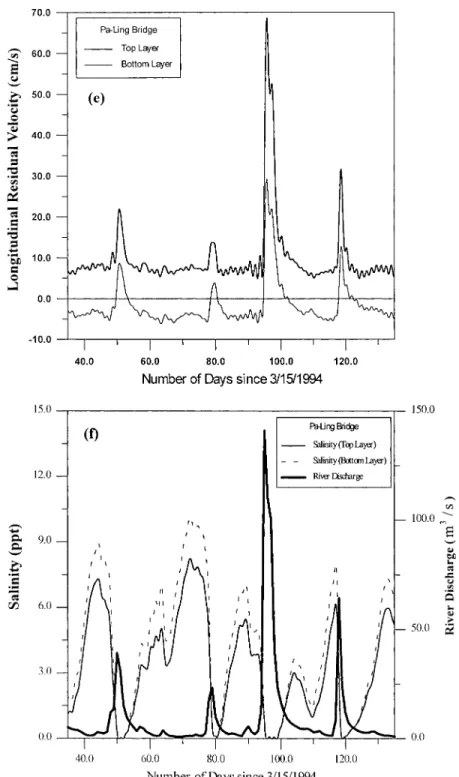
FIG. 3(a,b). Temporal Variations of Residual Velocity and Tidally Averaged Salinity at Kuan-Du Bridge Station

velocity and tidally averaged salinity. Fig. 3 presents the re-sidual velocities and tidally averaged salinities at three stations — Kuan-Du, Taipei Bridge, and Pa-Ling Bridge. Figs. 3(a), 3(c), and 3(e) show that residual currents at three stations were directed downriver near the surface and upriver near the bot-tom most of the time. The deviation from the characteristic two-layered circulation usually took the form of downriver flow at all depths, during high discharge events, with very strong downriver flow in the upper layer. The characteristic two-layered circulation prevailed for most of the time at Kuan-Du station. Though the pattern of two-layered circulation in the Tanshui River estuary was highly persistent, the strength of circulation was quite variable, mainly influenced by the freshwater discharge.

Figs. 3(b), 3(d), and 3(f) show that the tidally averaged sa-linity distributions exhibit vertical stratification during the

nor-mal flow condition. When freshwater discharge increases, the strong downriver flow not only depresses salinity throughout the estuary, but it also reduces the stratification as a result of increased vertical mixing and weakened two-layered circula-tion. Following a high discharge event, the salinity gradually returns to the normal conditions in a short period, normally less than 10 days.

EFFECT OF RIVER DISCHARGE

To investigate the response of the residual circulation to different levels of river discharges, a series of numerical ex-periments were conducted, each with constant river discharge. A harmonic tide of eight constituents at the river mouth was used to force the model. The eight constituents are M2(12.42 h), S2(12 h), N2(12.9 h), K1(23.93 h), O1(25.82 h), K2(11.97

JOURNAL OF WATERWAY, PORT, COASTAL, AND OCEAN ENGINEERING / MARCH/APRIL 2001 / 65

FIG. 3(c,d). Temporal Variations of Residual Velocity and Tidally Averaged Salinity at Taipei Bridge Station

h), P1 (24.07 h), and M4 (6.21 h). For the low flow case, the

model was run with the Q90freshwater discharges (a flow with

an exceedance probability of 0.90) of 4.0 m3

/s, 6.9 m3

/s, and 1.3 m3

/s at the upstream boundaries of the Tahan Stream, Hsin-tien Stream, and Keelung River, respectively. A constant sa-linity profile at the river mouth (based on the observation data of 25 and 27 ppt at the surface and bottom, respectively, with linear variation in the vertical direction) was used for the flood

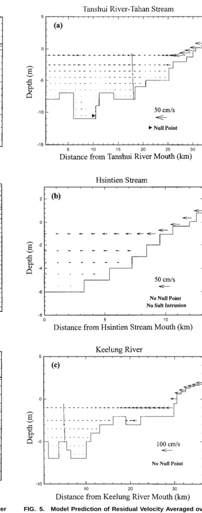
tide boundary condition. The average residual velocities over two spring-neap cycles, i.e., 29 days, are presented in Fig. 4, and indicate a general upriver residual flow along the bottom at the lower portions of all three rivers. There exists a null point at the upriver limit of the upriver bottom flow where bottom flows converge. The 1 ppt isohaline is also presented in the figure to indicate the limit of salt intrusion. Fig. 4 shows that the null point is located near the limit of salt intrusion in

66 / JOURNAL OF WATERWAY, PORT, COASTAL, AND OCEAN ENGINEERING / MARCH/APRIL 2001

FIG. 3(e,f). Temporal Variations of Residual Velocity and Tidally Averaged Salinity at Pa-Ling Bridge Station

the Tanshui River – Tahan Stream and the Hsintien Stream, while it is located some distance downstream of the limit of salt intrusion in the Keelung River. The relative locations of the null point and limit of salt intrusion in a partially mixed estuary have been demonstrated by Park and Kuo (1994) to vary, depending on the salinity gradient, water depth, and tid-ally averaged surface slope.

A moderate flow simulation was conducted using historical mean freshwater discharges of 62.1 m3

/s, 72.7 m3

/s, and 26.1 m3_{/s at the upstream boundaries of the Tahan Stream, Hsintien}

Stream, and Keelung River, respectively. All other conditions were kept the same as above. Fig. 5 shows that when the increased freshwater discharge pushes the limit of salt intru-sion downriver, the null point is also pushed downriver, but it moves farther than the limit of salt intrusion. The mean surface slope due to the freshwater discharge increases so much that

it requires a much stronger salinity gradient to generate upriver bottom flow.

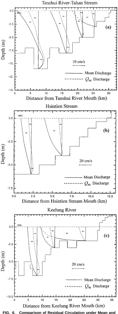
Fig. 6 compares the residual velocity profiles between Q90

and mean discharge conditions at various locations along the estuary. It shows that two-layered circulation exists in most parts of the Tanshui River – Tahan Stream and the lower por-tions of the tributaries under the low flow condition. Under the mean discharge condition, only the deeper, lower river sta-tion at Kuan-Du shows a two-layered circulasta-tion, with a weaker upriver flow than that under the low flow condition. This is contrary to the response in the much larger tributary estuaries of the Chesapeake Bay system, where the residual circulation strengthens with increasing freshwater discharge (Kuo et al. 1990; Park and Kuo 1996a).

Two physical processes are involved in the generation of residual velocity, which may be decomposed into two modes

JOURNAL OF WATERWAY, PORT, COASTAL, AND OCEAN ENGINEERING / MARCH/APRIL 2001 / 67

FIG. 4. Model Prediction of Residual Velocity Averaged over Two Spring-Neap Cycles with Q90Freshwater Discharge: (a)

Tan-shui River–Tahan Stream; (b) Hsintien Stream; (c) Keelung River

FIG. 5. Model Prediction of Residual Velocity Averaged over Two Spring-Neap Cycles with Historical Mean Freshwater Dis-charge: (a) Tanshui River–Tahan Stream; (b) Hsintien Stream; (c) Keelung River

68 / JOURNAL OF WATERWAY, PORT, COASTAL, AND OCEAN ENGINEERING / MARCH/APRIL 2001 FIG. 6. Comparison of Residual Circulation under Mean and

Q90Freshwater Discharges: (a) Tanshui River–Tahan Stream; (b)

Hsintien Stream; (c) Keelung River

of flow — barotropic and baroclinic. The barotropic flow is forced by the surface slope. The baroclinic flow is forced by the horizontal density (salinity) gradient. The magnitudes of these two modes may be calculated from model simulation results.

The forcing mechanisms of the residual circulation in an estuary can be expressed as ⫺1/␳ ⭸p/⭸x, where x = distance seaward along the river axis;␳ = water density; and p = pres-sure. In the following discussion, all dependent variables are tidally averaged quantities. The pressure gradient can be de-composed into the barotropic and baroclinic terms; that is

␩

1⭸p 1 ⭸␳ ⭸␩

⫺ = g

冉 冕

冊

␳ ⭸x ␳ ⫺h⭸x ⭸x

where g = gravitational acceleration; z = distance upward in the vertical direction; h = water depth at mean sea level; and

␩ = position of the free surface above mean sea level. Water

density can be expressed by an equation of state as

␳ = ␳ (1 ⫹ ks)0 (2)

where s = salinity; ␳0 = freshwater density; and k = constant

relating density to salinity (=7.5⫻ 10⫺4/ppt). Eqs. (1) and (2) are combined; applying Boussinesq’s approximation, then

␩

1 ⭸p ⭸s ⭸␩

⫺ = k

冕

␳g ⭸x ⫺h⭸x ⭸x

In (3),⭸␩/⭸x represents the barotropic mode and k兰⫺h␩ ⭸s/⭸x dz

is the baroclinic mode.

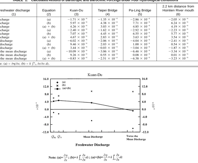
Table 1 presents the calculated results of these two modes for four hydrological conditions (Q90, Q75, mean discharge, and

twice the mean discharge) at various locations along the bot-tom of the estuary. The Q75 discharges at the tidal limits of

the three major tributaries are 8.15 m3_{/s, 20.2 m}3_{/s, and 3.61}

m3

/s for the Tahan Stream, Hsintien Stream, and Keelung River, respectively. Table 1 shows that under Q75and Q90low

flow conditions the baroclinic mode is stronger than the barot-ropic mode at all four stations, resulting in upriver flow along the bottom, as shown in Fig. 6. Under the mean flow condition the barotropic flow is stronger than the baroclinic flow at all stations except the deeper, lower river station at Kuan-Du. The residual upriver flow is driven by the integrated longitudinal salinity gradient; therefore, it increases with both depth and salinity gradient. Consequently, the residual upriver flow tends to be stronger in deeper sections of the estuary and in regions where the salinity gradient is large. Fig. 7 presents the varia-tion of forcing funcvaria-tions at Kuan-Du stavaria-tion with freshwater discharge. This figure shows that the net forcing, which drives the bottom water upriver, increases with river discharge at low flow. It also shows that even though the baroclinic forcing increases as the freshwater discharge increases from Q90to the

mean discharge, the barotropic forcing increases more; thus, the net forcing decreases and the strength of upriver flow is reduced. In the much larger estuaries of the Chesapeake Bay system, the barotropic forcing has much less response to an increase in river discharge. Therefore, the strength of estuarine circulation generally increases with river discharge, except during severe flood conditions (Kuo et al. 1990). The cessation of two-layered circulation at moderately high flow implies a weak trapping capacity in the Tanshui River estuary.

SPRING-NEAP VARIATIONS

To examine the response of residual circulation to the spring-neap cycle of tidal variation, the model simulation us-ing Q75flow was further examined. The computed time series

of velocity and salinity were averaged over two tidal cycles during periods of spring and neap tides, respectively. Fig. 8

JOURNAL OF WATERWAY, PORT, COASTAL, AND OCEAN ENGINEERING / MARCH/APRIL 2001 / 69

TABLE 1. Calculated Results of Barotropic and Baroclinic Forcings under Four Hydrological Conditions

Freshwater discharge (1) Equation (2) Kuan-Du (3) Taipei Bridge (4) Pa-Ling Bridge (5) 2.2 km distance from Hsintien River mouth

(6) Q90discharge (a) ⫺1.71 ⫻ 10⫺6 ⫺1.35 ⫻ 10⫺6 ⫺2.86 ⫻ 10⫺6 ⫺2.05 ⫻ 10⫺6 Q90discharge (b) 5.97⫻ 10⫺6 4.38⫻ 10⫺6 7.71⫻ 10⫺6 6.24⫻ 10⫺6 Q90discharge (a)⫹ (b) 4.26⫻ 10⫺6 3.03⫻ 10⫺6 4.85⫻ 10⫺6 4.19⫻ 10⫺6 Q75discharge (a) ⫺2.40 ⫻ 10⫺6 ⫺1.62 ⫻ 10⫺6 ⫺2.92 ⫻ 10⫺6 ⫺2.23 ⫻ 10⫺6 Q75discharge (b) 7.07⫻ 10⫺6 4.45⫻ 10⫺6 6.55⫻ 10⫺6 5.77⫻ 10⫺6 Q75discharge (a)⫹ (b) 4.67⫻ 10⫺6 2.83⫻ 10⫺6 3.63⫻ 10⫺6 3.54⫻ 10⫺6

Mean discharge (a) ⫺6.02 ⫻ 10⫺6 ⫺2.06 ⫻ 10⫺6 ⫺4.04 ⫻ 10⫺6 ⫺2.41 ⫻ 10⫺6

Mean discharge (b) 9.46⫻ 10⫺6 2.03⫻ 10⫺6 1.00⫻ 10⫺6 0.54⫻ 10⫺6

Mean discharge (a)⫹ (b) 3.44⫻ 10⫺6 ⫺0.03 ⫻ 10⫺6 ⫺3.04 ⫻ 10⫺6 ⫺1.87 ⫻ 10⫺6 Twice the mean discharge (a) ⫺10.09 ⫻ 10⫺6 ⫺3.06 ⫻ 10⫺6 ⫺6.46 ⫻ 10⫺6 ⫺3.34 ⫻ 10⫺6 Twice the mean discharge (b) 9.26⫻ 10⫺6 0.55⫻ 10⫺6 0.08⫻ 10⫺6 0.01⫻ 10⫺6 Twice the mean discharge (a)⫹ (b) ⫺0.83 ⫻ 10⫺6 ⫺2.51 ⫻ 10⫺6 ⫺6.38 ⫻ 10⫺6 ⫺3.23 ⫻ 10⫺6

Note: (a) =⭸␩/⭸x; (b) = k兰 ⭸s/⭸x dz.␩⫺h

FIG. 7. Magnitudes of Barotropic and Baroclinic Forcings as Functions of Freshwater Discharge

compares residual velocity profiles during spring and neap tides. It indicates that two-layered circulation exists in all three tributaries, as well as in the mainstream Tanshui River. Fig. 8 also shows that the spring tide has weaker residual circulation than does the neap tide. The result is similar to that for the larger estuaries of the Chesapeake Bay system (Park and Kuo 1996a). The more intense turbulent mixing during spring tide enhances the vertical momentum exchange, and thus reduces the residual circulation. On the other hand, the enhanced lon-gitudinal salinity gradient during spring tide may increase re-sidual circulation as a result of shorter salt intrusion. The shortening of salt intrusion during spring tide has been argued by Geyer (1993) using the steady-state momentum and salt balance equations, and shown using field data from the Co-lumbia River (Jay and Smith 1990) and data from a tidal flume (Rigter 1973). However, the response of the longitudinal sa-linity distribution tends to have a longer time scale than the change in tidal mixing over the spring-neap cycles, so its effect is greatly reduced (Fischer 1980). In the case of the Tanshui River, the model results show that the reduction in residual circulation by stronger tidal mixing during spring tide is more pronounced.

DISCUSSION AND CONCLUSIONS

A mathematical model is applied to study the hydrodynam-ics in the Tanshui River estuary in Taiwan. The model is a

laterally integrated, two-dimensional, real-time model. The hy-drodynamic model, which provides real-time predictions of surface elevation, current velocity, and transport of salt, has been validated using observational data collected in 1994 and 1995. The residual circulation in the estuary has been validated by comparing model results with theoretical analysis and field data (Hsu et al. 1999).

An investigation of long-term transport using the model vides further insight into the understanding of physical pro-cesses. The model results were filtered to arrive at the subtidal or tidally averaged quantities. A characteristic two-layered cir-culation prevails throughout most of the estuary under low flow conditions, e.g., Q90and Q75. The downriver directed

ba-rotropic forcing is smaller than the upriver directed baroclinic forcing, resulting in upriver flow along the river bottom at all stations investigated. As freshwater discharge increases, the barotropic forcing increases throughout the estuary, while the baroclinic forcing responds differently at various stations. The baroclinic forcing decreases at the upriver stations where sa-linity is low. At the downriver stations, particularly at Kuan-Du, where salinity is high and water depth is large, baroclinic forcing increases with freshwater discharge at lower flow, then decreases at higher flow, resulting in a nonmonotonic response of the residual circulation to freshwater discharge. Similar be-havior was observed in the larger tributary estuaries of the Chesapeake Bay system. However, in that system the barot-ropic forcing was much less sensitive to freshwater discharge,

70 / JOURNAL OF WATERWAY, PORT, COASTAL, AND OCEAN ENGINEERING / MARCH/APRIL 2001 FIG. 8. Model Prediction of Residual Velocity during Spring

and Neap Tides: (a) Tanshui River–Tahan Stream; (b) Hsintien Stream; (c) Keelung River

and two-layered circulation was observed even at very high flow (flood) conditions. In the Tanshui River, the two-layered circulation ceases to exist at moderately high flow. This has a significant long-term transport implication in the Tanshui River estuary, which is less of a ‘‘material trap’’ than most larger estuaries. The accumulated materials in the system will be flushed frequently.

The distinction between the limit of salt intrusion and the limit of gravitational circulation, the null point, was also ex-amined. Both are pushed downriver by the increase of fresh-water discharge; however, the null point is pushed farther than the limit of salt intrusion. The null point occurs where the longitudinal density gradient integrated over the total depth (baroclinic) balances the mean surface slope due to the fresh-water discharge (barotropic). With the increased barotropic forcing due to increased freshwater discharge, it requires stronger baroclinic forcing at a higher salinity region to counter the downriver flow. The response of residual velocity to the spring-neap cycle indicates stronger residual circulation during neap tide than spring tide. The spring tide provides more turbulent mixing energy and, thus, weaker velocity shear. All of these features were well reproduced by the model. ACKNOWLEDGMENTS

The project under which this study is conducted is supported by the National Science Council, Taiwan, under grant numbers NSC 88-2611-E-002-036 and NSC 89-2213-E-002-075. The financial support is highly appreciated. The writers also would like to express their appreciation to the manuscript reviewers; through their comments, this paper was sub-stantially improved.

APPENDIX I. REFERENCES

Chang, R. C., and Shi, T. T. (1989). ‘‘An investigation of tidal charac-teristics in the lower Tanshui River.’’ Geographic Studies, 13, 1–55 (in Chinese).

Fischer, K. (1980). ‘‘Salinity intrusion models.’’ Modelling of estuarine physics: Lecture notes on coastal and estuarine studies, Vol. 1, J. Sun-dermann and K. P. Holx, eds., Springer, New York, 232–241. Geyer, W. R. (1993). ‘‘How does variation in vertical mixing affect the

estuarine circulation?’’ Proc., 12th Int. Estuarine Res. Fedn. Conf. Hansen, D. V., and Rattray, M. Jr. (1965). ‘‘Gravitational circulation in

straits and estuaries.’’ J. Marine Res., 23, 104–121.

Hsu, M. H. (1998). ‘‘The influence on hydrodynamics in the Tanshui River system due to flood protection policy at Kuan-Du plain and Sheh-Tse Island.’’ Tech. Rep. No. 308, Hydrotech Research Institute, National Taiwan University, Taipei, Taiwan (in Chinese).

Hsu, M. H., Kuo, A. Y., Kuo, J. T., and Liu, W. C. (1996). ‘‘Study of tidal characteristics, estuarine circulation and salinity distribution in Tanshui River system (1).’’ Tech. Rep. No. 239, Hydrotech Research Institute, National Taiwan University, Taipei, Taiwan (in Chinese). Hsu, M. H., Kuo, A. Y., Kuo, J. T., and Liu, W. C. (1997). ‘‘Study of

tidal characteristics, estuarine circulation and salinity distribution in Tanshui River system (2).’’ Tech. Rep. No. 273, Hydrotech Research Institute, National Taiwan University, Taipei, Taiwan (in Chinese). Hsu, M. H., Kuo, A. Y., Kuo, J. T., and Liu, W. C. (1999). ‘‘Procedure

to calibrate and verify numerical models of estuarine hydrodynamics.’’ J. Hydr. Engrg., ASCE, 125(2), 166–182.

Hsu, S. S. (1969). ‘‘A study of the tidal unsteady flow in the lower Tanshui River.’’ Water Conservancy, 7, 38–49 (in Chinese).

Ianniello, J. P. (1977). ‘‘Tidally-induced residual currents in estuaries of constant breadth and depth.’’ J. Phys. Oceanography, 35(4), 755–786. Ianniello, J. P. (1981). ‘‘Comments on tidally induced residual currents in estuaries: Dynamics and near-bottom flow characteristics.’’ J. Phys. Oceanography, 11, 126–134.

Jay, D. A., and Smith, J. D. (1990). ‘‘Residual circulation in shallow estuaries. 1: Highly stratified, narrow estuaries.’’ J. Geophys. Res., 95, 711–731.

Kuo, A. Y., Hamrick, J. M., and Sisson, G. M. (1990). ‘‘Persistence of residual currents in the James River Estuary and its application to mass transport.’’ Residual currents and long-term transport: Coastal and es-tuarine studies, R. T. Cheng, ed., Springer, New York, 389–401. Kuo, A. Y., and Park, K. (1995). ‘‘A framework for coupling shoals and

shallow embayments with main channels in numerical modeling of coastal plain estuaries.’’ Estuaries, 18(2), 341–350.

JOURNAL OF WATERWAY, PORT, COASTAL, AND OCEAN ENGINEERING / MARCH/APRIL 2001 / 71 Ouyang, C. F. (1971). ‘‘Investigation of water pollution and

self-purifi-cation in the Tanshui River.’’ Taiwan Water Conservancy, 19(3), 67– 77 (in Chinese).

Park, K., and Kuo, A. Y. (1993). ‘‘A vertical two-dimensional model of estuarine hydrodynamics and water quality.’’ Spec. Rep., Appl. Marine Sci. and Oc. Engrg., Rep. No. 321, Virginia Institute of Marine Science, Gloucester Point, Va.

Park, K., and Kuo, A. Y. (1994). ‘‘Numerical modeling of advective and diffusive transport in the Rappahannock Estuary, Virginia.’’ Estuarine and Coast. Modeling III: Proc., 3rd Int. Conf. on Estuarine and Coast. Modeling, M. L. Spauding et al., eds., ASCE, Reston, Va., 461–474. Park, K., and Kuo, A. Y. (1996a). ‘‘Effect of variation in vertical mixing

on residual circulation in narrow, weakly nonlinear estuaries.’’ Buoy-ancy effects on coastal and estuaries dynamics: Coastal and estuarine studies, D. G. Aubrey and C. Friedrichs, eds., American Geophysical Union, Washington, D.C., 301–317.

Park, K., and Kuo, A. Y. (1996b). ‘‘A numerical model study of hypoxia in the tidal Rappahannock River of Chesapeake Bay.’’ Estuarine, Coast. and Shelf Sci., 42(5), 563–581.

Pritchard, D. W. (1956). ‘‘The dynamic structure of a coastal plain es-tuary.’’ J. Marine Res., 15, 33–42.

Pritchard, D. W. (1960). ‘‘The movement and mixing of contaminants in tidal estuaries.’’ Waste disposal in the marine environment, E. A. Pear-son, ed., Pergamon, Tarrytown, N.Y., 512–525.

Rigter, B. P. (1973). ‘‘Minimum length of salt intrusion in estuaries.’’ J. Hydr. Div., ASCE, 99(9), 1475–1496.

Water Resource Planning Commission. (1989). ‘‘Harmonic analysis of tidal elevations at Shy-Tzyy-Tour and Tu-Ti-Kung-Pi in the Tanshui River’’ (in Chinese).

Yen, C. L., and Hsu, M. H. (1982). ‘‘Numerical simulation of unsteady flow in river system.’’ Hydr. Rep. No. 7105, Civil Engineering Depart-ment, National Taiwan University, Taipei, Taiwan (in Chinese). APPENDIX II. NOTATION

The following symbols are used in this paper: g = gravitational acceleration;

h = water depth;

k = constant relating density to salinity (=7.5 ⫻ 10⫺4/ppt);

p = pressure; s = salinity;

x = distance seaward along river axis; z = distance upward in vertical direction;

␩ = position of free surface above mean sea level; ␳ = water density; and