網路攻防情境中之存活度分析與優化

行政院國家科學委員會專題研究計畫 成果報告

網路攻防情境中之存活度分析與優化

研究成果報告(精簡版)

計 畫 類 別 ： 個別型 計 畫 編 號 ： NSC 95-2221-E-002-168- 執 行 期 間 ： 95 年 08 月 01 日至 96 年 07 月 31 日 執 行 單 位 ： 國立臺灣大學資訊管理學系暨研究所 計 畫 主 持 人 ： 林永松 計畫參與人員： 碩士班研究生-兼任助理：臧柏皓、曾中蓮、林義倫、陳怡 孜、陳俊維、江坤道、溫雅芳、郭承賓 處 理 方 式 ： 本計畫可公開查詢

中 華 民 國 96 年 12 月 17 日

國

國

科

科

會

會

專

專

題

題

研

研

究

究

計

計

畫

畫

成

成

果

果

報

報

告

告

撰

撰

寫

寫

格

格

式

式

一、說明 國科會基於學術公開之立場，鼓勵一般專題研究計畫主持人發表其研 究成果，但主持人對於研究成果之內容應負完全責任。計畫內容及研究成 果如涉及專利或其他智慧財產權、違異現行醫藥衛生規範、影響公序良俗 或政治社會安定等顧慮者，應事先通知國科會不宜將所繳交之成果報告蒐 錄於學門成果報告彙編或公開查詢，以免造成無謂之困擾。另外，各學門 在製作成果報告彙編時，將直接使用主持人提供的成果報告，因此主持人 在繳交報告之前，應對內容詳細校對，以確定其正確性。 本格式說明僅為統一成果報告之格式，以供撰寫之參考，並非限制研 究成果之呈現方式。精簡報告之篇幅（不含封面之頁數）以 4 至 10 頁為原 則，完整報告之篇幅則不限制頁數。 成果報告繳交之期限及種類（精簡報告、完整報告或期中報告等），應 依本會補助專題研究計畫作業要點及專題研究計畫經費核定清單之規定辦 理。 二、內容格式：依序為封面、中英文摘要、目錄（精簡報告得省略）、報告內 容、參考文獻、計畫成果自評、可供推廣之研發成果資料表、附錄。 (一)報告封面：請至本會網站（http：//www.nsc.gov.tw）下載製作（格式如附 件一）。 (二)中、英文摘要及關鍵詞(keywords)。 (三)報告內容：請包括前言、研究目的、文獻探討、研究方法、結果與討論 （含結論與建議）…等。若該計畫已有論文發表者，可以 A4 紙影印， 作為成果報告內容或附錄，並請註明發表刊物名稱、卷期及出版日 期。若有與執行本計畫相關之著作、專利、技術報告、或學生畢業論 文等，請在參考文獻內註明之，俾可供進一步查考。 (四)頁碼編寫：請對摘要及目錄部分用羅馬字 I 、II、 III……標在每頁下 方中央；報告內容至附錄部分請以阿拉伯數字 1.2.3.……順序標在每頁 下方中央。 (五)附表及附圖可列在文中或參考文獻之後，各表、圖請說明內容。 (六)計畫成果自評部份，請就研究內容與原計畫相符程度、達成預期目標情 況、研究成果之學術或應用價值、是否適合在學術期刊發表或申請專 利、主要發現或其他有關價值等，作一綜合評估。 (七)可供推廣之研發成果資料表：凡研究性質屬

應用研究

及

技術發展

之計 畫，請依本會提供之表格（如附件二），每項研發成果填寫一份。 三、計畫中獲補助國外或大陸地區差旅費、出席國際學術會議差旅費或國際合 作研究計畫差旅費者，須依規定撰寫心得報告（出席國際學術會議者須另附 發表之論文），以附件方式併同成果報告繳交，並請於成果報告封面註記。 四、打字編印注意事項 1. 用紙 使用A4 紙，即長 29.7 公分，寬 21 公分。

2. 格式

中文打字規格為每行繕打（行間不另留間距），英文打字規格為 Single

Space。 3. 字體

報告之正文以中英文撰寫均可。在字體之使用方面，英文使用 Times

行政院國家科學委員會補助專題研究計畫

ˇ成果報告

□期中進度報告

網路攻防情境中之存活度分析與優化

計畫類別：ˇ 個別型計畫 □ 整合型計畫

計畫編號：NSC95－2221－E－002－168－

執 行 期 間 ： 95 年 8 月 1 日至 96 年 7 月 31

日

計畫主持人：林永松博士

共同主持人：

計畫參與人員：

成果報告類型(依經費核定清單規定繳交)：□精簡報告 □完整報告

本成果報告包括以下應繳交之附件：

□赴國外出差或研習心得報告一份

□赴大陸地區出差或研習心得報告一份

□出席國際學術會議心得報告及發表之論文各一份

□國際合作研究計畫國外研究報告書一份

處理方式：除產學合作研究計畫、提升產業技術及人才培育研究計

畫、列管計畫及下列情形者外，得立即公開查詢

□涉及專利或其他智慧財產權，□一年□二年後可公開查

詢

附件一

執行單位：國立台灣大學資訊管理學系

一、計畫中文摘要 [中文關鍵字] 拉格蘭日鬆弛法、網路攻擊與防禦、最佳化問題、資源配置策略、存活 度 自從美國發生 9/11 恐怖攻擊事件之後，如何以效果與效率兼備的方式，保護重要 基礎建設(特別是網際網路)，已成為一個重要的資訊安全(Information Security)議題。 由於攻擊事件發生的必然性，網際網路是很難達到完美的強固性(Robustness)。為充分 描述一個系統如何在處於不正常的情況下(包括發生隨機錯誤或遭受惡意攻擊)，還能 夠維持正常服務運作的程度，近幾年來對於資訊安全的概念逐漸被延伸成為存活度 (Survivability)的觀念。 為了有效提升網路遭到惡意攻擊後的存活度，網路營運者(防守者)必須對其所管控 之網路，投資一筆固定的預算(例如：金錢、時間、人力)，並加以妥善配置，用以建 立強固的安全防禦機制；另一方面，攻擊者所擁有的資源亦是有限的，其不可能攻擊 那些所需成本超過自身能負擔的網路。因此，潛在的攻擊者也會因應網路營運者所採 用的資源配置策略(Resource Allocation Strategy)，調整其攻擊策略(Attack Strategy)，俾 便以最少的攻擊成本達成預定之攻擊目的。

然而，目前並沒有相關研究，係運用數學規劃法(Mathematical Programming)等最佳 化(Optimization)技巧，針對資訊安全中的網路攻防問題(Network Attack and Defense)， 從網路營運者的觀點，來探討如何配置有限的資源，以提升網路存活度，並嚇阻攻擊 者進行攻擊，進而降低整體網路風險。本研究計畫將率先處理此問題，並提出三個數 學模型。

二、計畫英文摘要

Keywords: Lagrangean Relaxation, Network Attack and Defense, Optimization Problem, Resource Allocation Strategy, Survivability

Since the 9/11 terrorist attacks in the United States, the effective and efficient protection of critical information infrastructures, especially the Internet, has become an even more important issue. With the inevitability of such attacks, perfect robustness of the Internet is unobtainable; hence, in recent years, the concept of security has been increasingly generalized as an issue of survivability. Since there are only two states, safe and compromised, in the context of security, the concept is definitely insufficient to fully describe how a system can sustain normal services under abnormal conditions, including random errors and malicious attacks. Consequently, the issue of survivability has drawn increasing attention in recent years.

To enhance network survivability effectively, a network operator must invest a fixed amount of budget (e.g. money, time, and manpower) and distribute it properly. On the other hand, an attacker also has limited resource to launch an attack, so he won’t choose to compromise a network if the incurred attack cost exceeds his acceptable level. Thus, a potential attacker will always adjust his strategies to compromise a network at minimal cost, if he knows the defense resource allocation strategy of the network operator. For that reason, a network operator’s budget allocation strategy should consider that an attacker will constantly adjust his strategy to attain his goals. It is therefore a major challenge for network operators to derive adequate defense strategies against attacks. However, there has been no theoretical research that would enable network operators to gain a global understanding of how to allocate limited budgets to network components so that the survivability of their networks can be maximized to deter attackers’ intrusions.

However, there has been little research on the issues of defense and attack based on mathematical programming models. Moreover, to the best of our knowledge, no mathematical model that deals with defense and attack behavior in the context of survivability has been proposed. In this project, we therefore propose three mathematical models that fully describe the conflict between an attacker and a defender, and show different levels of network survivability for given defense resource allocation strategies. We then analyze the problem with optimization-based models, in which the problem structure is, by nature, a mixed integer programming problem.

三、報告內容

(一) Y.-S. Lin, P.-H. Tsang, C.-H. Chen, C.-L. Tseng, and Y.-L. Lin, “Evaluation of Network Robustness for Given Defense Resource Allocation Strategies,” Proceedings of the 1st

International Conference on Availability, Reliability and Security (ARES’06), pp. 182-189,

April 2006.

Abstract

Since the 9/11 terrorist attacks, the effective and efficient protection of critical information infrastructures has become an even more important issue. To enhance network survivability, a network operator needs to invest a fixed amount of budget and distribute it properly. However, a potential attacker will always adjust his attack strategies to compromise a network at minimal cost, if he knows the resource allocation strategy of the network operator. In this paper, we first evaluate the survivability of a given network under two different metrics; that is, we assess the minimal attack cost incurred by an attacker. The two survivability metrics are assumed to be the connectivity of at least one given critical Origin-Destination pair (OD pair) and that of all given critical OD pairs. We then analyze the problem with two optimization-based models, in which the problem structure is, by nature, a mixed integer programming problem.

1. Introduction 1.1. Background

The 9/11 terrorist attacks in the United States have led to an increasing global focus on security, especially the effective and efficient protection of infrastructures that are critical to our society. Specifically, the Internet has become a critical information infrastructure since the 1990s. By applying security mechanisms under the defense-in-depth strategy [1], we can enhance the level of robustness. However, the robustness of a network depends not only on each component’s resistance to malicious attacks, but also the network’s topological structure. The Internet’s topology has been shown to follow a power-law degree distribution [2], and the empirical evidence has highlighted one major weakness: the Internet is highly susceptible to malicious attacks.

With the inevitability of such attacks, perfect robustness of the Internet is unobtainable; hence, in recent years, the concept of security has been increasingly generalized as an issue of

survivability. Since there are only two states, safe and compromised, in the context of

security [3], the concept is definitely insufficient to fully describe how a system can sustain normal services under abnormal conditions, including random errors and malicious attacks. Consequently, the issue of survivability has drawn increasing attention in recent years [4, 5].

1.2. Related works of Survivability

Despite the rapid increase in survivability research, the definition of survivability is anything but clear [6]. Since it is impossible, in practice, to build a perfectly survivable network, it is important to be able to quantitatively evaluate the efficacy of a network that is believed to be survivable. From our survey, methods that attempt the quantitative analysis of survivability can be classified into two categories: connectivity or performance.

Factor (NCF) [7] and the Link Connectivity Factor (LCF) [8]. The former deals with the removal of nodes, while the latter is concerned with the removal of links. Several methodologies can be used to analyze the connectivity of networks. Among them, linear/non-linear programming [8] and simulation with given metrics [7] are the most popular.

In general, network performance is analyzed by calculating the probability that the network will fulfill its given QoS metrics. Because of the variety of network performance metrics, many diverse methodologies, such as Markov chain [5], game theory [9] and simulation with given metrics [10], can be used for analysis.

1.3. Motivation and objectives of this paper

To enhance network survivability effectively, a network operator must invest a fixed amount of budget (e.g. money, time, and manpower) and distribute it properly. On the other hand, an attacker also has limited resource to launch an attack, so he won’t choose to compromise a network if the incurred attack cost exceeds his acceptable level. Thus, a potential attacker will always adjust his strategies to compromise a network at minimal cost, if he knows the defense resource allocation strategy of the network operator.

In this paper, to understand how well a network can sustain malicious attacks, we evaluate the minimal attack cost incurred by an attacker who attempts to disconnect critical Origin-Destination pair(s) (OD pair(s)). The concept of attack cost relates to the effort an attacker needs to make to attain his goal. However, to the best of our knowledge, no mathematical model that deals with defense and attack behavior in the context of survivability has been proposed. We therefore propose two mathematical models that fully describe the conflict between an attacker and a defender, and show different levels of network survivability for given defense resource allocation strategies. Briefly, Model 1 deals with the disconnection of at least one critical OD pair in a network, while Model 2 addresses the disconnection of all critical OD pairs in a network.

1.4. Outline of this paper

The remainder of this paper is organized as follows. In Section 2, a min mathematical formulation of an attack-defense scenario is proposed, which is later shown to be a trivial problem. In Section 3, another min mathematical formulation of an advanced attack-defense scenario is proposed, for which a Lagrangean Relaxation-based solution approach is presented. In Section 4, the computational results of the second formulation are reported. Finally, in Section 5, we present our conclusions.

2. Problem formulation for model 1

2.1. Problem descriptions and assumptions

The evaluation of the robustness of a network under malicious attack is modeled as an optimization problem, in which the objective is to minimize the total attack cost from an attacker’s perspective, such that at least one given critical OD pair is disconnected and the network cannot survive.

In this model, we assume that both the attacker and the defender have complete information about the targeted network topology. Moreover, the attacker has complete information about the defender’s budget allocation. For simplicity, we only consider node

attacks, which result in the worst case scenarios and are more common in the real world. We now define the notations used in this paper and formulate the problem.

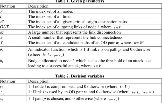
Table 1. Given parameters

Notation Description

V The index set of all nodes

L The index set of all links

W The index set of all given critical origin-destination pairs

OUT i The index set of outgoing links of node i, where i V∈

M A large number that represents the link disconnection ε A small number that represents the link connectedness

w

P The index set of all candidate paths of an OD pair w, where w W∈

δpl An indicator function, which is 1 if link l is on path p, and 0 otherwise

(where l L∈ , p P∈ _w)

bi Budget allocated to node i, which is also the threshold of an attack cost

leading to a successful attack, where i V∈

Table 2. Decision variables

Notation Description

yi 1 if node i is compromised, and 0 otherwise (where i V∈ )

wl

t 1 if link l is used by an OD pair w, and 0 otherwise (where l L∈ , w W∈ )

xp 1 if path p is chosen, and 0 otherwise (where p P∈ w)

l

c Cost of link l, where l L∈

Objective function: min i i i y

∑

_{i V∈} y b , (IP 1) subject to l i c =y M+ε _{∀ ∈i V l OUT}, _∈ i _{(IP 1.1)} wl l pl l l L l L t c δ c ∈ ∈ ≤

∑

∑

∀ ∈p P w W_w, ∈ (IP 1.2) w p pl wl p P x δ t ∈ =

∑

∀ ∈w W l L, ∈ (IP 1.3) wl l l L w W M t c ∈ ∈ ≤

∑ ∑

(IP 1.4) 1 w p p P x ∈ =

∑

∀ ∈w W (IP 1.5) 0 or 1 p x = ∀ ∈p P w W_w, ∈ (IP 1.6) 0 or 1 i y = ∀ ∈i V (IP 1.7) 0 or 1 wl t = ∀ ∈w W l L, _{∈ (IP 1.8)} or l c =ε M +ε ∀ ∈l L. _{(IP 1.9)}

The objective of this formulation is to minimize the total attack cost. Constraint (IP 1.1) describes the definition of the link cost, which is ε if the link functions normally, and M+ε if it is broken. Constraint (IP 1.2) requires that the selected path for each OD pair, w, should be the minimum cost path. Constraint (IP 1.3) is the relation among twl, xp and δpl. We use the

requires that at least one critical OD pair is disconnected. We depict the phenomenon by showing that the sum of the shortest path costs for each OD pair to communicate is greater than M. Constraint (IP 1.9) is a set of redundant constraints, since the value of each cl should

be either εor M+ε.

Argument 1 We can relax the equality of Constraint (IP 1.1) as cl ≤y Mi +ε without affecting

the optimality conditions.

Argument 2 We can relax the equality of Constraint (IP 1.3) as w

p pl wl p P xδ t ∈ ≤ ∑ _{without affecting}

the optimality conditions.

2.2. Solution to model 1

Lemma 1 Given a budget allocation strategy, a topology, G= (V, L), and a set of critical OD

pairs, W, the formulation of Model 1 can be optimally solved by combining the maximum flow-minimum cut algorithm [11] and the node splitting method [11] within time complexity O(|W|¯(|V|+|L|)¯n), where n is the total budget allocated to the network.

Proof. The maximum flow-minimum cut algorithm finds the minimum link cost that

separates the network into two subsets, where the origin node belongs to subset S and the destination node belongs to subset S. With the node splitting method, on the other hand, a node can be converted into a link by dividing it into two independent subnodes and introducing an artificial link to connect the subnodes. By assuming that the link capacity between two subnodes of a node is the given budget (i.e., the attack cost) of the node and other links’ capacities are infinite, we first transform G(V, L) into G’(V’, L’). Using the maximum flow-minimum cut algorithm, the minimum cost of separating G’ into two subsets for OD pair w, where w W∈ , can then be denoted by MCTw, which is also the minimum cut for OD pair w in G’. Since the network contains |W| critical OD pairs, we can find the minimum cost for each OD pair after running the maximum flow-minimum cut algorithm |W| times. Thus, the solution to Model 1 is min(MCTw), where w W∈ . Meanwhile, the time complexity of the maximum flow-minimum cut algorithm is O((|V|+|L|)¯n), and the time complexity of solving Model 1 optimally is O(|W|¯(|V|+|L|)¯n), where n is the total capacity (not including the infinite capacity), i.e., the total defense budget, of the network.

3. Problem formulation for model 2

3.1 Problem descriptions and assumptions

We now consider another scenario of the attack-defense problem. Assume that an attacker must disconnect all given critical OD pairs to compromise a network.

The given parameters and decision variables of Model 2 are the same as those of Model 1, except that a new given parameter, B, which is the total budget of a defender, is introduced. The objective of this formulation (IP2) and the constraints (IP 2.1)~(IP 2.10) of Model 2 are the same as those for Model 1, except the two following constraints.

wl l l L M t c ∈ ≤

∑

∀ ∈w W (IP 2.4) i lb i V y V ∈ ≥

∑

(IP 2.10) Constraint (IP 2.4) requires that all critical OD pairs must be disconnected. We explain the phenomenon by showing that the cost of the shortest path for each OD pair to communicate is greater than M. Constraint (IP 2.10) is a redundant constraint. We find a legitimate lower

bound, Vlb, which is the number of nodes an attacker must target to compromise the

connectivity of all critical OD pairs.

Argument 3 The legitimate lower bound described in Constraint (IP 2.10) can be obtained by

the following method.

We assign one unit of the budget to each node. Then, we solve this revised optimization problem and find a lower bound of the Lagrangean Relaxation (LR) method [12], denoted by LB, on the optimal objective function value. LB indicates the minimal (but not necessarily feasible) cost an attacker must expend to achieve his goal. Since each node is assigned one unit of the budget, LB also serves as the lower bound of the number of nodes an attacker needs to compromise.

3.2. Solution to model 2

By applying the Lagrangean Relaxation method with a vector of Lagrangean multipliers, we can transform the problem of (IP2) into the following Lagrangean Relaxation problem (LR), where constraints (IP 2.1), (IP 2.2), (IP 2.3), and (IP 2.4) are relaxed.

Lagrangean Relaxation Problem

1 1 2 3 4 2 3 4 ( , , , ) min [ ( )] [ ] [( ) ] i i w w D _y i i il l i i V i V l OUT wp wl l pl l wl p pl wl w wl l w W p P l L w W l L p P w W l L Z u u u u y b u c y M u t c c u x t u M t c ε δ δ ∈ ∈ ∈ ∈ ∈ ∈ ∈ ∈ ∈ ∈ ∈ = + − + + ⎡ ⎤ − + − + _⎢ − _⎥ ⎣ ⎦ ∑ ∑ ∑ ∑ ∑ ∑ ∑∑ ∑ ∑ ∑ (LR) subject to 1 w p p P x ∈ =

∑

∀ ∈w W (LR1) 0 or 1 p x = ∀ ∈p P w Ww, ∈ (LR2) 0 or 1 i y = ∀ ∈i V (LR3) 0 or 1 wl t = ∀ ∈w W l L, ∈ _(LR4) or l c =ε M+ε ∀ ∈l L _(LR5) . i lb i V y V ∈ ≥

∑

(LR6) By definition, u u u u1, , ,2 3 4 are the vectors of {u1il}, {u2wp}, {u3wl}, {u4w}, respectively. Note

that u u u u1, , ,2 3 4 are Lagrangean multipliers and u u u u1, , ,2 3 4≥0. To solve (LR) optimally, we

decompose it into the following three independent and easily solvable optimization subproblems.

Subproblem 1 SUB_1 (related to decision variable x_p)

3 1( ) min3 w sub wl pl p w W l L p P Z u u δ x ∈ ∈ ∈ =

∑ ∑ ∑

, (Sub 1) subject to (LR1) and (LR2).

This problem can further be decomposed into |W| independent minimum cost path subproblems. In other words, we can determine the value of xp individually for each OD pair.

Due to the non-negativity constraint of each u3

wl, which can be treated as the cost of link l in

OD pair w in the minimum cost path subproblems, we can apply Dijkstra’s shortest path algorithm to solve these subproblems optimally. The time complexity of SUB_1 is

Subproblem 2 SUB_2 (related to decision variable y_i) 1 2( ) min1 ( ) i sub i i il i i V i V l OUT Z u y b u M y ∈ ∈ ∈ =

∑

+

∑ ∑

− , (Sub 2) subject to (LR3) and (LR6).

To solve SUB_2 optimally, we first apply the quick sort algorithm to the sum of the parameters of each yi to obtain an array in ascending order. To satisfy Constraint (LR6), we

choose Vlb nodes from the left of the array, and set their yi values to one. The yi values of the

remaining nodes are decided by their associated parameters. If it is positive, the value of yi is

set to zero to minimize this subproblem; otherwise, it is set to one. The time complexity of SUB_2 is O(|V|log|V|).

Subproblem 3 SUB_3 (related to decision variables ,t c_{wl l})

1 2 3 1 2 3 4 3 4 ( , , , ) min ( ) ( ) ( ) i w sub il l wp wl l pl l i Vl OUT w W p P l L wl wl w wl l w W l L w W l L Z u u u u u c u t c c u t u t c δ ∈ ∈ ∈ ∈ ∈ ∈ ∈ ∈ ∈ = + − + − + −

∑ ∑

∑ ∑ ∑

∑∑

∑

∑

(Sub 3) subject to (LR4) and (LR5).

As Constraints (LR4) and (LR5) show, twl and cl have two combinations each. We can

therefore apply an exhaustive search to determine the values of twl and cl, depending on which

combination derives the smallest objective function value. To optimally solve SUB_3, we further decompose it into |L| independent subproblems. The time complexity of SUB_3 is O(|W|¯|L|).

According to the weak Lagrangean duality theorem [12], the optimal value of the Lagrangean Relaxation (LR) problem is, by nature, a lower bound (for minimization problems) of the objective function value in the primal problem. The tightest Lagrangean lower bound can be derived by tuning the Lagrangean multipliers, i.e., by maximizing the LR problem. There are several methods for solving this problem, of which the Subgradient optimization technique [13] is the most popular.

Getting Primal Feasible Solutions

To obtain the primal feasible solutions of (IP2), we consider the solutions of the LR problem. By using the Lagrangean Relaxation method and the Subgradient method to solve the LR problem, we not only get a theoretical lower bound on the primal objective function value, but also obtain good hints for getting primal feasible solutions. However, as some critical and difficult constraints are relaxed to obtain the easily-solvable LR problem, the solutions obtained from ZD may not be valid for the primal problem. Thus, we need to develop good heuristics to tune the values of the decision variables, so that primal feasible solutions can be obtained. Our proposed heuristics are as follows.

Table 3. Algorithm for getting a primal feasible solution

Sort the array of nodes in ascending order according to the associated parameters of yi in

SUB_2;

INIT all yi to 0;

FOR (each unexamined node i in the array with the smallest parameter) {

IF (there is an available path for at least one given critical OD pair to communicate)

IF (the parameter of yi < 0 OR the node’s outgoing link cost is greater than M)

}

/* recovery of the attack behavior to reduce ineffective attacks */

FOR (each attacked node i with the largest budget, bi) {

SET yi to 0;

IF (there is an available path for at least one given critical OD pair to communicate)

SET yi to 1;

}

FOR (any two combinations, i and j, of the attacked nodes) {

SET yi and yj to 0;

IF (there is an available path for at least one given critical OD pair to communicate)

SET yi and yj to 1;

}

The time complexity for getting primal heuristics is O(|W|¯|V|5).

4. Computational experiments

To demonstrate that our proposed solution to Model 2 is better than other approaches, we implement the following two simple algorithms for comparison.

4.1. Simple algorithm 1

Table 4. Simple algorithm 1 FOR (each OD pair)

Run Maximum Flow-Minimum Cut algorithm to get the minimum cuts;

FOR (each node that belongs to any of the minimum cuts AND contains at least one outgoing link labeled as M) {

Run Dijkstra’s Shortest Path algorithm under the node’s recovery;

IF (the recovery of the node is unallowable) Un-recover the node;

}

4.2. Simple algorithm 2

Table 5. Simple algorithm 2

Sort the nodes in descending order according to their degree of connectivity;

WHILE (there is an available path for at least one OD pair to communicate)

Attack the most connected node among those that have not been attacked;

4.3. Experimental parameters and cases

We present our experimental parameters and the design of cases in the following table.

Table 6. Experimental parameters

Number of Nodes 16, 50, 100

Number of Links 60 ~ 400

Number of Critical OD pairs 8 ~ 250 Testing Topology

Random Networks (RN) Grid Networks (GN)

Initial Budget Allocation Strategy Uniform Distribution, _{Degree-based Distribution} Number of Iterations 2000

Non-improvement Counter 80

Initial Upper Bound Solution of Simple Algorithm 1

4.4. Experimental results

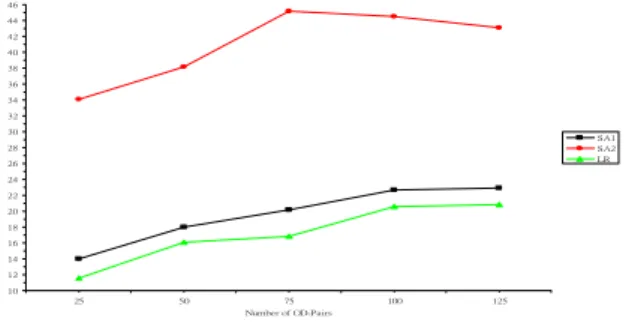
We present the experimental results in the appendix section and show the figures below. SA1 and SA2 are the solutions obtained by the Simple Algorithms 1 and 2; the LR value represents the primal feasible solution derived by the LR process; and LB represents the lower bound gained from the LR process. The duality gap is calculated by LR-LB*100%

LB . 10 12 14 16 18 20 22 24 26 28 30 32 34 36 38 40 42 44 46 25 50 75 100 125 Number of OD-Pairs A tta ck C os t SA1 SA2 LR

Figure 1. Medium-scale random networks

20 24 28 32 36 40 44 48 52 56 60 64 68 72 76 80 84 88 92 96 25 50 75 100 125 Number of OD-Pairs A ttac k C os t SA1 SA2 LR

Figure 2. Large-scale random networks

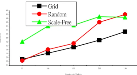
15 17 19 21 23 25 27 29 31 33 35 37 50 100 150 200 250 Number of OD-Pairs At tack C os t Grid Random Scale-Free

Figure 3. Effect of different topologies (large-scale networks with a uniform budget allocation strategy)

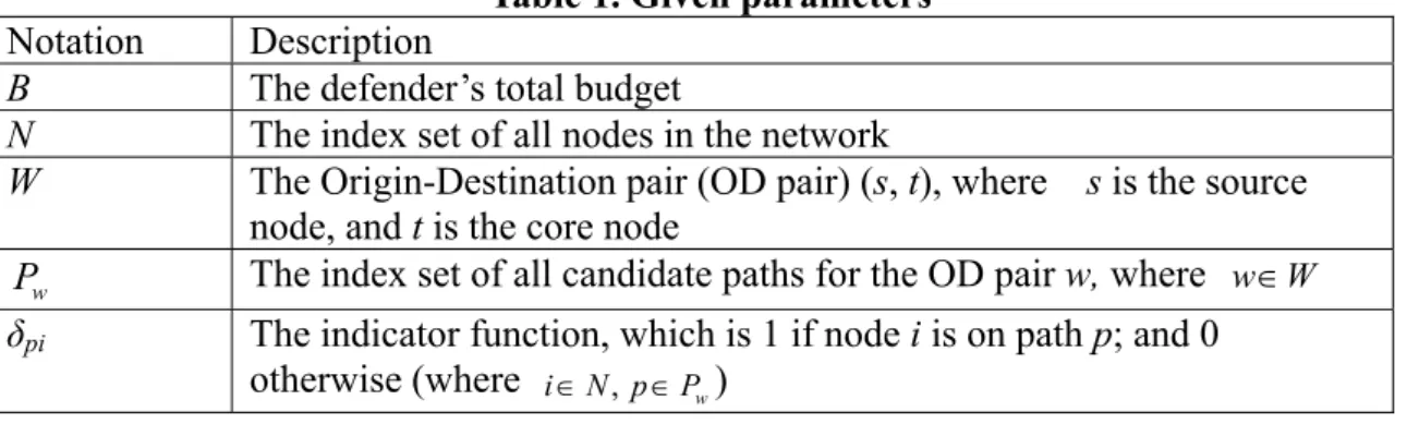
20 22 24 26 28 30 32 34 36 38 40 42 44 46 48 50 100 150 200 250 Number of OD-Pairs Attack C os t Grid Random Scale-Free

Figure 4. Effect of different topologies (large-scale networks with a degree-based budget allocation strategy)

4.5. Discussion

From Figures 1 and 2, we observe that the curves of the LR-based algorithms are all below those of SA1 and SA2, which means that the solution quality of LR is better than those of SA1 and SA2, because this is a minimization problem. Specifically, the solution excellence of the LR-based algorithm is demonstrated when a network’s size increases and more OD pairs are considered.

Since a legitimate lower bound of the primal objective function value (LB) can be obtained by Lagrangean Relaxation, we can also evaluate the solution quality of LR by comparing it with the LB. We find that even in a medium-scale network or large-scale network, the duality gap, in most cases, is less than 45%.

Moreover, we find that a network’s topological structure strongly influences its robustness against attack. Figure 3 shows the minimal attack costs of different network topologies under a uniform budget allocation strategy with the same network size and number of critical OD pairs. Clearly, cost of attacking a random network is greater than that of attacking a scale-free network. This indicates that the property of randomness may help maintain the connectivity of a network. The connectivity of a scale-free network is usually maintained by a few super nodes. However, since an attacker will try to destroy nodes that have a high degree of connectivity to achieve his goal more easily, the effect of destroying some super nodes would be significant. Therefore, the robustness of a scale-free network is weaker than that of a random network, since it can be shut down completely by compromising fewer nodes than in a random network.

If we compare Figure 3 with Figure 4, we can see that a proper budget allocation strategy enhances the robustness of a network. By adjusting the budget allocation strategy according to the degree of connectivity, a scale-free network can achieve the higher level of robustness than a random network most of the time, as shown in Figure 4. Thus, if we allocate proper budgetary resources to high-connectivity nodes, we can increase the costs incurred by an attacker.

5. Conclusions

In this paper, we have focused on two issues. First, we have discussed the robustness of a network and evaluated the minimal attack cost of an attacker based on two different survivability metrics: the connectivity of at least one OD pair, and the connectivity of all critical OD pairs. Second, we have presented one lemma, which shows a pseudo-polynomial time solution approach to solve Model 1 optimally.

One of the major contributions of our paper is the mathematical models. We have researched the problem characteristics carefully, identified the problem objectives and the

associated constraints, and proposed well-formulated mathematical models. To the best of our knowledge, this paper is the first to model attack-defense scenarios as mathematical programming problems in the context of survivability. Furthermore, we have provided solution approaches to find the minimal attack cost for both models, and derived a legitimate lower bound on the number of nodes an attacker would need to target in Model 2. The proposed lemma is another major contribution. After studying the problem structure of Model 1, we find trivial solution for the problem and present it as elegant lemma.

Finally, we have evaluated different topologies and observed their ability to maintain the connections of all critical OD pairs under malicious attack. The experimental results show that a random network can survive better than a scale-free network. However, with a proper budget allocation strategy, a scale-free network can achieve the higher level of robustness than a random network most of the time.

We believe that our modeling techniques can be extended to different attack-defense scenarios in the context of survivability in which the survivability metrics include “any number of given critical OD-pairs are disconnected,” “a single core node is survivable,” or “multiple core nodes are survivable.” Besides considering the state of a node is compromised or not merely, we could lead into the concept of probability to define the likelihood of a node being properly functional. We are also interested in the extent to which our methods can be extended to scenarios with the interactive dependency of network nodes, and specific application parameters of wireless networks, mobile phone networks, and other kinds of network environment.

References

[1] “Information Assurance Technical Framework (IATF) Release 3.1:2002”, National Security Agency (NSA), http://www.iatf.net/framework_docs/version-3_1/.

[2] Q. Chen, H. Chang, R. Govindan, S. Jamin, S. J. Shenker, and W. Willinger, “The Origin of Power Laws in Internet Topologies Revisited”, Proceedings of the 21th Annual Joint Conference of the IEEE Computer and Communications Societies (INFOCOM ’02),

Volume 2, 2002, pp. 608-617.

[3] R. J. Ellison, D. A. Fisher, R. C. Linger, H. F. Lipson, T. A. Longstaff, and N. R. Mead, “Survivable Network Systems: An Emerging Discipline”, Technical Report CMU/SEI-97-TR-013, Software Engineering Institute, Carnegie Mellon University, November 1997 (Revised: May 1999).

[4] J. C. Knight, E. A. Strunk, and K. J. Sullivan, “Towards a Rigorous Definition of Information System Survivability”, Proceedings of the DARPA Information Survivability

Conference and Exposition (DISCEX 2003), Volume 1, April 2003, pp.78-89.

[5] Y. Liu and K. S. Trivedi, “A General Framework for Network Survivability Quantification”, Proceedings of the 12th GI/ITG Conference on Measuring, Modeling and Evaluation of Computer and Communication Systems, September 2004.

[6] V. R. Westmark, “A Definition for Information System Survivability”, Proceedings of

the 37th IEEE Hawaii International Conference on System Sciences, Volume 9, 2004, p.

90303.1.

[7] R. Albert, H. Jeong, and A.-L. Barabási, “Error and Attack Tolerance of Complex Networks”, Nature, Volume 406, July 2000, pp. 378-382.

[8] N. Garg, R. Simha, and W. Xing, “Algorithms for Budget-Constrained Survivable Topology Design”, Proceedings of the 2002 IEEE International Conference on

Communications, Volume 4, 2002, pp. 2162-2166.

Survivable and Secure Systems and Protocols”, Proceedings of the 2nd International Workshop on Mathematical Methods, Models, and Architectures for Computer Network Security, LNCS 2776, September 2003, pp. 440-443.

[10] W. Molisz, “Survivability Function—A Measure of Disaster-Based Routing Performance”, IEEE Journal on Selected Areas in Communications, Volume 22, Issue 9, November 2004, pp. 1876-1883.

[11] R. K. Ahuja, T. L. Magnanti, and J. B. Orlin, Network Flows, 1993, pp. 41-42, 184-191, 598-648.

[12] M. L. Fisher, “The Lagrangean Relaxation Method for Solving Integer Programming Problems”, Management Science, Volume 27, Number 1, January 1981, pp. 1-18.

[13] M. Held, P. Wolfe, and H. P. Crowder, “Validation of Subgradient Optimization”,

Mathematical Programming, Volume 6, 1974, pp. 62-88.

[14] A.-L. Barabasi and R. Albert, “Emergence of Scaling in Random Networks”, Science, Volume 286, October 1999, pp. 509-512.

Appendix

Case 1: Small-scale (16-node) networks with degree-based budget distribution

Network

Topology No. of Critical OD pairs SA1 SA2 LR LB Duality Gap

8 4.33 16 4.33 4.1286 4.88% 16 7.33 16 7.33 6.639864 10.40% 24 7.33 16 7.33 6.833638 7.26% 32 10.33 16 10.33 9.147548 12.93% Grid Networks 40 12.33 16 12.33 10.2583 20.20% 8 5.2 9.8 5.066667 4.363142 16.51% 16 7.4 12.93333 6.8 5.579946 21.81% 24 8.266667 14.46667 7.866667 6.813326 16.22% 32 9.666666 14.26667 9.066666 7.604745 19.43% Random Networks 40 9.2 15 9 7.820135 14.88% 8 6.62069 11.2 6.179311 5.118475 21.79% 16 8.331034 13.46207 7.944828 6.760865 18.26% 24 8.827586 13.68276 8.717241 7.424418 17.60% 32 10.2069 14.12414 9.875862 7.924543 25.12% Scale-free Networks 40 10.48276 14.78621 10.26207 8.535546 20.32%

Case 2: Medium-scale (50-node) networks with degree-based budget distribution

Network

Topology No. of Critical OD pairs SA1 SA2 LR LB Duality Gap

25 13.23912 39.52071 11.66706 8.67917 34.39% 50 22.22557 41.89881 19.73563 14.72979 34.14% 75 21.29319 46.7002 19.60321 13.89132 41.15% 100 19.52173 43.6905 18.89996 14.45762 31.03% Grid Networks 125 21.01724 47.04804 20.29598 14.99273 35.42% 25 14 14 11.6 9.531583 21.68% 50 18 18 16.06667 12.88349 24.76% 75 20.2 20.2 16.8 13.47968 24.81% 100 22.66667 22.66667 20.6 16.81728 22.84% Random Networks 125 22.93333 22.93333 20.8 16.36455 27.22% 25 15.56701 37.62887 14.94845 12.38963 21.05% 50 22.62887 42.42268 19.79381 16.06501 23.91% 75 25.05155 42.78351 22.83505 17.6532 29.75% 100 25.30928 45.36082 23.71134 19.00001 24.76% Scale-free Networks 125 26.64948 43.29897 25.46392 20.68265 23.29%

Case 3: Large-scale (100-node) networks with degree-based budget distribution

Network

Topology No. of Critical OD pairs SA1 SA2 LR LB Duality Gap

50 32.84444 94.7 23.10222 16.52974 39.78% 100 32.63335 96.52222 26.21112 18.65637 40.56% 150 32.93333 97.17775 29.28888 20.88303 40.30% 200 38.11555 98.63332 32.84445 21.65815 51.87% Grid Networks 250 40.69554 95.20222 37.17778 23.6082 57.52% 50 29.4 56.93333 22.40465 17.7652 25.65% 100 35.2 83.66667 28.06667 21.54525 30.22% 150 37.26667 76.86667 31.2 24.18611 29.17% 200 47.2 93.2 42 29.81787 40.92% Random Networks 250 51.6 95.6 46 37.51661 22.65% 50 35.32995 78.4264 32.08122 24.07327 33.35% 100 44.77157 85.58376 40.05076 30.69447 30.62% 150 45.73604 83.85787 40.50761 30.70721 32.20% 200 49.3401 94.72081 44.8731 34.59037 29.84% Scale-free Networks 250 50.10152 97.96954 44.51777 35.32274 26.12%

(二) F.Y.-S. Lin, P.-H. Tsang, and Y.-L. Lin, "Near Optimal Protection Strategies against Targeted Attacks on the Core Node of a Network," Proceedings of the 2nd International Conference on Availability, Reliability and Security (ARES’07), pp. 213-222, April 2007.

Abstract

The issue of information security has attracted increasing attention in recent years. In network attack and defense scenarios, attackers and defenders constantly change their respective strategies. Given the importance of improving information security, a growing number of researchers are now focusing on how to combine the concepts of network survivability and protection against malicious attacks. As defense resources are limited, we propose effective resource allocation strategies that maximize an attacker’s costs and minimize the probability that the “core node” of a network will be compromised, thereby improving its protection. The two problems are analyzed as a mixed, nonlinear, integer programming optimization problem. The solution approach is based on the Lagrangean Relaxation method, which solves this complicated problem effectively. We also evaluate the survivability of real networks, such as scale-free networks.

1. Introduction

It has been shown that the Internet’s topology follows a power-law degree distribution [1] and is thus highly susceptible to malicious attacks [2]. As a result, the field of information security has attracted increasing attention in recent years, and a number of approaches have been proposed to protect networks against such attacks. Research shows that attackers and defenders constantly change their respective strategies – a process that can be likened to the use of a lance and a targe.

Network survivability is another important research domain. Initially, researchers focused on the effect of random failures on networks and tested the robustness and dependability of networks. However, given the need to constantly improve information security, researchers are now paying more attention to protection against malicious attacks and to combining the concept with the field of network survivability.

Many definitions, techniques, and architectures for evaluating a network’s survivability have been proposed. The most well-known definition is “the ability of a system to fulfill its mission in a timely manner, in the presence of attacks, failures, or accidents” [3]. Several of the definitions address the following key information security requirements: 1) the maintenance of service under attack; and 2) the provision of strategies to prevent attacks [4]. In this paper, we focus on the second requirement.

In addition to the above definitions of survivability, a number of models have been proposed to evaluate network survivability. For example, in [5], the authors describe several models that quantitatively evaluate survivability; and in [6], the state-based architecture proposed in [7] is adopted to quantitatively analyze survivability. The latter is implemented by a Markov chain. Meanwhile, because of the growing importance of information security, some researchers have started to focus on how to combine the concept of survivability with that of protection against malicious attacks. Thus in [8], the authors model attack-defense scenarios as mathematical programming problems in the context of survivability.

In this paper, we consider network survivability in terms of protection of the “core node” in which organizations store their most valuable knowledge. Because of the node’s importance, attackers do their best to compromise it; thus, defenders must change their strategies to protect the node against compromise by the constantly evolving strategies of attackers. As defense resources are limited, network operators need guidelines about how to

allocate security budgets effectively. To this end, we propose two mathematical models: the protection strategies for defenders (PSD) model and the probabilistic protection strategies for defenders (PPSD) model, to formulate attack-defense scenarios. Our objective is to provide defenders with effective defense resource allocation strategies to protect the core node, so that the cost of compromising the node would be unacceptable to an attacker.

The remainder of the paper is organized as follows. In Section 2, we propose the PSD model, and present a Lagrangean Relaxation-based solution approach for obtaining near optimal protection strategies. In Section 3, the second mathematical formulation, the PPSD model, is proposed. It is an extension of the PSD model and employs heuristics to calculate good primal feasible solutions. In Section 4, the results of computational experiments on the PSD and PPSD models are reported. Finally, in Section 5, we present our conclusions.

2. Problem formulation for the PSD model 2.1. Problem description and assumptions

To compromise a core node, an attacker must find a suitable path to it and compromise all the intermediate nodes on that path. However, compromising a node costs the attacker some resources, such as time, money, and man-power. From a defender’s perspective, if more defense resources are allocated to a node, its security will be improved and the attacker’s costs will be increased. However, since defense resources are limited, the defender must adopt an effective resource allocation strategy to maximize the attacker’s costs.

In the worst-case scenario, if the attacker can obtain complete information about the target network and use it intelligently, he will find the path with the minimal attack cost to

compromise the core node. Meanwhile, the defender will try to maximize the minimized attack cost through different budget allocation strategies. In response, the attacker will then search for another path with the minimal attack cost to compromise the core node.

Next, we define the notations used in this paper and formulate the problem.

Table 1. Given parameters

Notation Description

B The defender’s total budget

N The index set of all nodes in the network

W The Origin-Destination pair (OD pair) (s, t), where s is the source node, and t is the core node

w

P The index set of all candidate paths for the OD pair w, where w W∈

δpi The indicator function, which is 1 if node i is on path p; and 0

otherwise (where i N p P∈ , ∈ w)

Table 2. Decision variables

Notation Description

yi 1 if node i is compromised, and 0 otherwise (where i N∈ )

xp 1 if path p is chosen as the attack path, and 0 otherwise (where p P∈ w)

bi The budget allocated to protect node i, where i N∈

ˆ ( )_{i i}

a b The threshold of the attack power required to compromise node i, i.e., the defense capability of node i, where i∈N

( )

i i

Objective function: ˆ max min ( ) p i w i i p pi x b i N p P a b xδ ∈ ∈

∑

∑

, (IP 1) subject to: i i N b B ∈ ≤

∑

(1-1) 0≤ ≤ b_i B i N∈ (1-2) 1 w p p P x ∈ =

∑

(1-3) 0 1 p x = or p P∈ w. (1-4)

The objective function is to maximize the minimized total attack cost, where the defender manipulates the budget to maximize the total attack cost, while the attacker tries to minimize that cost by choosing a suitable attack path. To simplify the original problem, we reformulate it as follows: Objective function: ˆ min ( ) i i i i b i N y a b ∈ −

∑

, (IP 2) subject to: ˆ( ) ˆ ( ) i i i pi i i i N i N y a b δ a b ∈ ∈ ≤

∑

∑

p P∈ w (2-1) w p pi i p P xδ y ∈ ≤

∑

i N∈ (2-2) 1 w p p P x ∈ = ∑ (2-3) 0 1 p x = or p P∈ w (2-4) 0 1 i y = or i N∈ (2-5) i i N b B ∈ ≤

∑

(2-6) 0≤ ≤ b_i B i N∈ . (2-7)

We reformulate the objective function (IP 1) as one of minimizing the attacker’s negative attack cost, i.e., (IP 2). Constraint (2-1) requires that the selected path for the OD pair should be the minimum attack cost path. Constraint (2-2) is the relation between yi, xp and δpi. We

use the auxiliary set of decision variables, yi, to replace the product of xp and δpi, which

further simplifies the problem-solving procedures. Other constraints are straightforward.

2.2. Solution for the PSD model

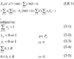
By applying the Lagrangean Relaxation method [9] with a vector of Lagrangean multipliers u1 and u2, we can transform the reformulation of the PSD model into the following Lagrangean Relaxation problem (LR 1). In this case, Constraints (2-1) and (2-2) are relaxed. Furthermore, we assume that a bˆ ( )_{i i} is equal to the concave function ln(bi+1), which

indicates that the marginal defense capability of node i can be reduced by allocating additional budget.

1 2 1 1 2 ( , ) min ln( 1) ( )ln( 1) ( w w D i i i N p i pi i i p pi p p i N i N p P Z u u y b u y δ b u xδ y ∈ ∈ ∈ ∈ ∈ = − + + − + + − ∑ ∑ ∑ ∑ ∑ , (LR 1) subject to: 1 w p p P x ∈ =

∑

(3-1) 0 1 p x = or _{p P∈ w} (3-2) 0 1 i y = or i N∈ (3-3) i i N b B ∈ ≤

∑

(3-4) 0≤ ≤ b_i B i N∈ . (3-5)

To solve (LR 1) optimally, we decompose it into the following two independent and easily solvable optimization subproblems.

Subproblem 1-1 (related to decision variable xp)

2 min w i p pi i N p P u x δ ∈ ∈

∑ ∑

, (SUB 1-1) subject to (3-1) and (3-2).

(SUB 1-1) can be viewed as a minimum cost path problem with node weight 2

i pi

u δ . Because 2

i

u is non-negative, we can apply Dijkstra’s shortest path algorithm to solve it

optimally. The time complexity is O(|N|2).

Subproblem 1-2 (related to decision variables yi, bi)

1 1 2 min ( 1) ln( 1) ln( 1) w w p i i p pi i i i p p i N p p i N i N u y b uδ b u y ∈ ∈ ∈ ∈ ∈ − + − + −

∑

∑

∑ ∑

∑

, (SUB 1-2) subject to (3-3), (3-4), and (3-5).

To solve (SUB 1-2) optimally, we adopt some mathematical techniques to carefully choose proper values for the random variables bi and yi. The time complexity is O(|N|2).

Based on the weak Lagrangean duality theorem [9], the optimal value of problem (LR 1) is, by its nature, the lower bound (for minimization problems) of the objective function value in the primal problem. We try to obtain the tightest lower bound of (LR 1) by applying the subgradient optimization technique proposed in [10] to tune the Lagrangean multipliers. Getting primal feasible solutions

Information provided by the multipliers is very helpful in deriving a heuristic that can solve the problem (IP 2). In this case, the multiplier vector 2

i u is adjusted by the function ( i pi) ( )ˆi i i N y δ a b ∈ −

∑ , which indicates the relative importance of each node i. This gives us a hint about how to allocate the budget. Our proposed heuristic is described in Table 3.

Table 3. Algorithm for getting a primal feasible solution for the PSD model

Step 1 Construct a minimal defense region by applying the labeling and the removal processes. The labeling process is based on a breadth-first search, and the removal process tests whether each outer layer node is

necessary.

Step 2 _{Allocate bi to each node, where} 2 2 ~ , to tal i i i i u b r i N u = ∈ . If a node has 0 i

r > , and it is not in the minimal defense region, allocate its budget to

the source and destination nodes.

Step 3 Tune the epsilon budget from the source and core nodes to the other nodes in the minimal defense region. If the value of the objective function is less than that of the previous state, we continue the tuning process recursively.

The time complexity of the heuristic is O(|N|2).

3. Problem formulation for the PPSD model 3.1 Problem description and assumptions

Based on the PSD model, we assume there is a probability that each node can be compromised, and that attacks on nodes are independent. Therefore, from an attacker’s perspective, the probability that a core node can be compromised successfully is the aggregate of the compromise probability of all nodes on the attack path between the source node and the core node. A defender can reduce a node’s compromise probability by allocating more defense resources to it. However, because such resources are limited, the defender needs to adopt a strategy that allocates the defense budget effectively in order to minimize the possibility of the core node being compromised.

In the worst-case scenario, if the attacker can obtain complete information about the target network and can use it intelligently, he will try to find the least secure path to compromise the core node, i.e., the path on which the aggregate of the compromise probability of all nodes is maximal. Meanwhile, the defender will try to improve the network’s security by allocating a different budget to each node.

Objective function: min ln ( ) i i i i b

∑

_{i N∈} P b y , (IP 4) subject to: ln ( )i i i ln ( )i i pi i N i N P b y P b δ ∈ ∈ − ≤ −

∑

∑

p P∈ w (4-1) w p pi i p P x δ y ∈ ≤

∑

i N∈ (4-2) 1 w p p P x ∈ =

∑

(4-3) 0 1 p x = or p P∈ _w (4-4) 0 1 i y = or i N∈ (4-5) i i N b B ∈ ≤

∑

(4-6) 0≤ ≤ b_i B i N∈ . (4-7)

To simplify this problem, we transform the compromise probability Pi(bi) of each node i

minimize the weight of compromising the core node. Constraint (4-1) requires that the selected path for the OD pair should be the path with the minimal weight.

3.2. Solution to the PPSD model

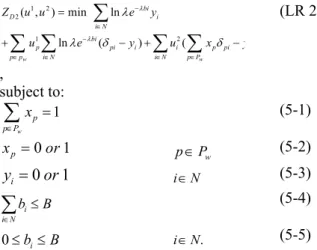
By applying the Lagrangean relaxation method with a vector of Lagrangean multipliers u1 and u2, we can transform the PPSD model into the following Lagrangean relaxation problem (LR 2). In this case, Constraints (4-1) and (4-2) are relaxed.

Furthermore, we assume that Pi(bi) follows an exponential distribution with λ, which

indicates that the compromise probability will be rapidly reduced by the additional budget allocated to a node. We can decompose the optimization problem (LR 2) into the following two independent subproblems and solve them optimally.

Subproblem 2-1 (related to decision variable xp)

2 min w i p pi i N p P u x δ ∈ ∈

∑ ∑

, (SUB 2-1) subject to (5-1) and (5-2). Because 2 i

u is non-negative, we can apply Dijkstra’s shortest path algorithm to solve

(SUB 2-1) optimally. The time complexity is O(|N|2).

Subproblem 2-2 (related to decision variables yi, bi)

1 1 2 min (1 ) ln ln w w bi bi p i p i i p p i N p p i N i N u λe−λ y u λe−λ δ u y ∈ ∈ ∈ ∈ ∈ −

∑ ∑

+

∑ ∑

−

∑

, (SUB 2-2) subject to (5-3), (5-4), and (5-5).

To solve (SUB 2-2) optimally, we use mathematical techniques to determine the proper values of the random variables bi and yi. The time complexity is O(|N|).

Getting primal feasible solutions

Using the method for getting primal feasible solutions for the PSD model, we derive a heuristic for the PPSD model, as shown in Table 4.

Table 4. Algorithm for getting a primal feasible solution for PPSD model

Step 1. Construct a minimal defense region by applying the labeling and the removal processes. The labeling process is based on a breadth-first search, and the

1 2 2 1 2 ( , ) min ln ln ( ) ( w w bi D i i N bi p pi i i p pi p p i N i N p P Z u u e y u e y u x y λ λ λ λ δ δ − ∈ − ∈ ∈ ∈ ∈ = + − + −

∑

∑ ∑

∑ ∑

, (LR 2) subject to: 1 w p p P x ∈ =

∑

(5-1) 0 1 p x = or _{p P∈ w} (5-2) 0 1 i y = or i N∈ (5-3) i i N b B ∈ ≤

∑

(5-4) 0≤ ≤ b_i B i N∈ . (5-5)

removal process tests whether each outer layer node is necessary. Step 2. _{Allocate bi to each node, where} 2

2 ~ , to ta l i i i i u b r i N u = ∈ . If a node has 0 i

r > , and it is not in the minimal defense region, allocate its budget to the source or destination nodes, depending on which one has the larger λ value. Step 3. Tune the epsilon budget from the source and core nodes to the other nodes that

have the highest negative value of the objective function in the minimal defense region. If the value of the objective function is less than that of the previous state, we continue the tuning process recursively.

Step 4. Compare with the primal-based heuristic, which allocates the budget to each node according to the value of the primal variable bi. Then, we determine the minimal objective value of the heuristics.

The time complexity of the heuristic is O(|N|3).

4. Computational experiments 4.1 Experiment environments

In the PSD model, we assume that a bˆ ( )_{i i} is the same for each node in a homogenous network.

To evaluate the PPSD model, we consider two scenarios. In scenario 1, following the 20/80 rule, we assume that 20% of the nodes in the network are more important than the other 80%. Therefore, we assume that the Pi(bi) for 20% of the nodes follows an exponential distribution

with a smaller λ(λ1) value; and for the other 80%, the Pi(bi) follows an exponential

distribution with a larger λ(λ2) value. Note that λ represents the initial compromise probability

of each node.

In scenario 2, we assume that the Pi(bi) for an OD pair follows an exponential distribution

with a randomly selected λ value between [0, 0.5]. Because the source node and the core node are important, we assume that the OD pair has a certain level of protection initially. For the other nodes, we assume that Pi(bi) follows an exponential distribution with a randomly

selected λ value between [0, 1].

We use two simple algorithms and one primal-based heuristic to compare the attack costs of different defense resource allocation strategies with those of our proposed algorithms. Simple algorithm 1 (SA1) allocates bi uniformly. In simple algorithm 2 (SA2), however, the

allocation of bi is proportionate to the ratio Links of a node

Total # of Links. In the primal-based heuristic

(HE3), the budget allocation for each node is based on the value of the primal variable bi,

which is derived by solving (SUB 1-2).

We discuss the experiment results in the next two subsections and present them in tabulated form in the Appendix. The LR value represents the primal feasible solution derived by the LR process; and LB represents the lower bound gained from the LR process. The duality gap is calculated by LB-LR

*100%

LR , and the survivability factor is calculated by

L R L B .

Finally, we transform the objective value into a positive to simplify the explanation

Grid Networks 0 10 20 30 16 49 100 225 361 Nodes A ttack C os t LR SA1 SA2 HE3

Figure 1. Attack costs in grid networks

Scale-Free Networks 0 0.5 1 16 49 100 225 361 Nodes Su rv iv ab ility LR SA1 SA2 HE3

Figure 2. Survivability of scale-free networks

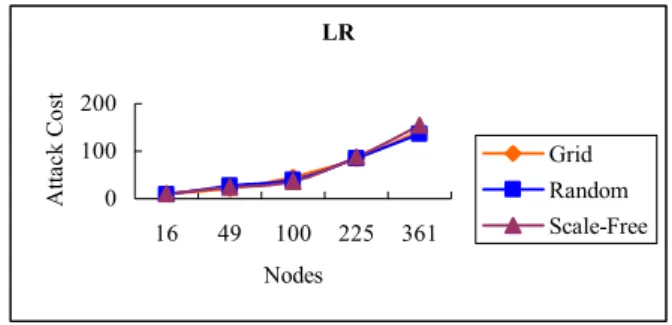
LR 0 10 20 30 16 49 100 225 361 Nodes A ttack C os t Grid Random Scale-Free

Figure 3. Effect of different network topologies

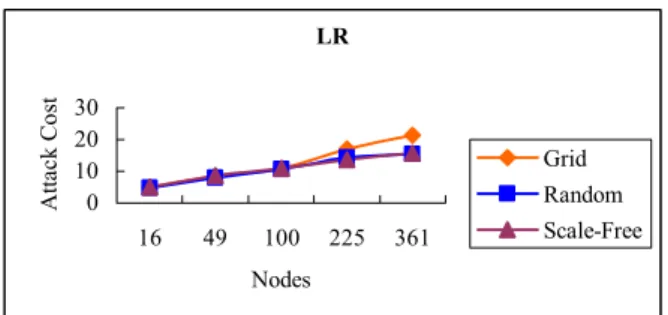
In Figure 1, the attack costs incurred by our proposed algorithm (Table 3) are always higher than those of the other algorithms used for comparison. The efficacy of the LR-based algorithm’s solution is clearly demonstrated as the size of the network increases. Figure 2 shows that the survivability factor of the proposed algorithm is consistently higher than that of the other algorithms. Thus, by applying the algorithm, the core node will be more robust and secure. Meanwhile, Figure 3 demonstrates that a network’s topological structure strongly influences its robustness against attack. The attack costs in large grid networks are higher than those in large random and scale-free networks [2]. The reason is that the average number of nodes that must be compromised in a grid network is higher than in a random or scale-free network. This is due to the small-world phenomenon [2]. Therefore, we can conclude that the defense-in-depth strategy [11] is an important factor in network survivability.

4.3 Experiment results for the PPSD model

The experiment results for scenario 1 of the PPSD model are similar to the results of the PSD model in Figures 1, 2, and 3. The proposed algorithm (Table 4) incurs higher attack costs than the two simple algorithms, and maintains a higher level of survivability in different-sized network topologies. We observe that, if the values of λ1 and λ2 are similar, the

LR 0 50 100 150 16 49 100 225 361 Nodes A ttack C os t Grid Random Scale-Free

Figure 4. Attack costs of scenario 1 of the PPSD model: different network topologies

(λ1=0.2, λ2=0.8)

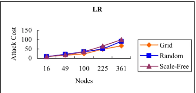
However, if λ1 is different to λ2, we must consider the specific characteristics of each node,

such as its importance on the path and its Pi(bi) function. For example, a node with a

substantial number of links that provide short cuts from the source node to the core node is very important in a scale-free network. If this kind of node is vulnerable (especially if its λ value is high), more defense resources should be allocated to it in order to reduce the risk of it being compromised. Because the effect of a node’s characteristics is greater than that of the defense-in-depth strategy, the attack costs in scale-free networks are higher than those in the other two network topologies, especially if the network is large, as shown in Figure 4.

Scale-Free Networks 0 100 200 16 49 100 225 361 Nodes A ttack C os t LR SA1 SA2

Figure 5. Attack costs in scenario 2: scale-free networks Random Networks 0 0.5 1 16 49 100 225 361 Nodes Su rv iv ab ility LR SA1 SA2

LR 0 100 200 16 49 100 225 361 Nodes A ttack C os t Grid Random Scale-Free

Figure 7. Attack costs of different network topologies in scenario 2

In scenario 2 of the PPSD model, the curves of the LR-based algorithms are all above those of SA1 and SA2. Thus, the solution quality of LR is better than that of SA1 or SA2, as shown in Figures 5 and 6, respectively. Considering both the defense-in-depth concept and the nodes’ characteristics, the attack costs incurred by the proposed algorithm are approximately equal in different-sized network topologies, as shown in Figure 7. This implies that the proposed protection strategy is very adaptive such that we can obtain almost the same result in networks of different size and topology.

5. Conclusion

We have focused on two issues. First, to improve the security of the core node in a network, we have proposed two mathematical models to formulate attack-defense scenarios and provide defenders with useful defense resource allocation strategies. Second, we have considered network survivability and evaluated the maximal minimized attack costs in different scenarios.

The mathematical models represent the major contribution of this work. We have carefully researched the security problem’s characteristics, identified its objectives and associated constraints, and proposed well-formulated mathematical models to solve it. To the best of our knowledge, the proposed approach is one of the few that model attack-defense scenarios as mathematical programming problems in the context of survivability. In addition, we have provided solution approaches to determine the attack costs for both models.

Finally, our evaluation of different topologies revealed the following phenomenon. In a homogeneous network, the defense-in-depth strategy is the most important issue to be considered when allocating a defense budget. Because a grid network does not contain short cuts, the attacker must compromise more nodes than in random or scale-free networks. Therefore, a defender can employ nodes with more levels when allocating defense resources in a grid network, which means that an attacker must expend further resources to compromise the core node. However, if a network is heterogeneous, the defender must pay more attention to each node’s characteristics. In random and scale-free networks, the nodes that provide short cuts are the most vulnerable. Therefore, we allocate more budget resources to them to improve the protection of the core node. The greater the differences between the nodes, the stronger will be the impact of each node’s characteristics. The proposed solution approach is not only very effective, it is also adaptable to different attack/defense scenarios.

We believe that the proposed models can be extended to different attack-defense scenarios in the context of survivability, where the survivability metrics include “the percentage of critical OD pairs disconnected,” “the number of core nodes that are survivable in a multiple core node environment,” or “the percentage of valuable information not stolen.” In our future work, we will investigate the extent to which our methods can be applied to scenarios involving the interactive dependency of network nodes. We will also examine specific