計算解剖學之腦區域擷取與對位演算法

國

立

交

通

大

學

資訊科學與工程研究所

博

士

論

文

計算解剖學之腦區域擷取與對位演算法

Brain Extraction and Registration Algorithms

for Computational Anatomy

研 究 生：劉嘉修

指導教授：陳永昇 博士

Brain Extraction and Registration Algorithms

for Computational Anatomy

研 究 生：劉嘉修 Student：Jia-Xiu Liu

指導教授：陳永昇 Advisor：Yong-Sheng Chen

國 立 交 通 大 學

資 訊 科 學 與 工 程 研 究 所

博 士 論 文

Submitted to Institute of Computer Science and Engineering College of Computer Science

National Chiao Tung University in partial Fulfillment of the Requirements

for the Degree of Doctor of Philosophy

in

Computer Science

December 2009

Hsinchu, Taiwan, Republic of China

謝謝永昇老師及麗芬老師 除了生活上的照顧與學業上的指導外 老師對研究的熱誠更是影響我甚深的無形教誨 謝謝李石增醫師、江安世老師、盧鴻興老師、荊宇泰老師及林益如老師 所給予的建議與對疏漏處的指正讓論文內容更臻詳實 謝謝常被我遙控的清偉、億婷及實驗室的學弟妹們 謝謝所有關心我的人 謝謝

計算解剖學（computational anatomy）廣泛運用非侵入式造影與影像處理方 法於腦部結構分析上。為讓結構分析聚焦於腦組織並使腦結構空間標準化，腦區 域擷取（brain extraction）與腦部結構對位（brain registration）在計算解剖學上 扮演重要之角色。此兩項技術之準確性可提升結構分析之可信度，且其高執行效 率可增加結構分析之處理容量進而提升統計效度。本論文針對快速且準確之腦部 結構分析提出腦區域擷取與腦部對位演算法，並將所開發之影像處理技術運用於 躁鬱症病患之腦纖維病理分析上。 在腦區域擷取方法中，本論文提出新的隱式形變模型（implicit deformable model）以期能有效的切割出腦部區塊。我們採用一組具區域影響性之 Wendland 輻射基底函數（radial basis function）以描述平滑的腦部曲線，並降低隱式形變 模型之計算複雜度。在內力（internal force）與外力（external force）的交互作用 下，輻射基底函數中心點將依次由初始位置逐漸推進至腦部邊界。由於不同視角 下的腦部邊界曲率往往差異頗大，因此我們分別對矢狀面（sagittal view）與冠狀 面（coronal view）的影像切片進行腦部區域擷取，並將不同切面的擷取結果整 合以達到互補之效果。利用 Internet Brain Segmentation Repository 兩組測試影像 所進行的效能評估結果，顯示本論文所提出的腦部擷取技術較 Brain Surface Extractor、Brain Extraction Tool、Hybrid Watershed Algorithm 與 Model-based Level Set 等方法有更佳的準確性與強健性（robustness）。 在腦結構影像對位方面，我們藉由影像導數（image derivatives）所得到的腦 結構資訊，以仿射轉換（affine transformation）與非線性形變模型建立測試影像 與目標影像間的空間對應關係。利用腦結構方向性之不同與腦重心位置之差異可 估計一組旋轉角度與位移量，以作為仿射對位的初始值。承續仿射對位之空間對 應結果，所提出的非線性方法階層式的將 Wendland 輻射基底函數佈置於具顯著 腦結構的區域上以描述影像的形變，仿射轉換與非線性形變均以階層式之影像解 析度進行影像相似度之最佳化。一般而言，非線性最佳化（nonlinear optimization） 結果之優劣深受初始值之影響。而本論文所提出之方法能有效的估計仿射對位與 非線性對位的初始空間對應關係。運用多組高解析度與低解析度影像之效能評估 結果，顯示所提出的影像對位方法較許多已廣泛運用的演算法精準且快速。另外， 本論文亦以模擬影像實驗量化影像對位準確度對腦結構分析正確性之影響。 雖然罹患第一型與第二型躁鬱症（bipolar disorders）之病患呈現相異的表徵 與認知能力（cognitive functions），然而此二亞型（subtypes）是否亦具有不同之 神經基質（neural substrates）卻一直是未知的。為探究第一與第二型躁鬱症病患 間之腦部纖維結構性差異，我們運用所開發之影像處理技術以及由擴散張量磁振 造影（diffusion tensor imaging）所導出之非等向性指標（fractional anisotropy） 於正常人、第一型躁鬱症病患、第二型躁鬱症病患與所有躁鬱症病患間之腦部纖

型躁鬱症病患的腦部纖維均在視丘（thalamus）、前扣帶（anterior cingulate）與 下額頁（inferior frontal）等位置有顯著性之結構異常。另外，第二型躁鬱症病患 的腦部纖維損傷現象亦呈現於顳頁（temporal）及下前額頁（inferior prefrontal） 等區域。第一型躁鬱症的右下額頁與第二型躁鬱症的左中顳頁等區域之平均非等 向性指標與認知執行功能具顯著性相關，第二型之躁鬱症病患的左中顳頁與下前 額頁等區域之平均非等向性指標與楊氏躁症量表（YMRS）分數及輕躁症發作期 （hypomanic episodes）呈顯著性相關。此研究結果指出第一型躁鬱症病患的腦 纖維異常處多與認知功能有關，而第二型躁鬱症病患具顯著性差異之位置則涵括 了認知與情緒處理等功能。 本論文提出兼具高執行效率與高準確度之腦部擷取與腦結構對位等演算法， 所提出之影像處理方法的高準確性可使結構分析結果更值得信賴；而其低計算複 雜度可使需要大量運用腦部擷取與腦結構對位的結構分析更有效率。本論文亦將 所開發的影像處理方法運用於分析躁鬱症病患的腦部纖維結構之損傷，此結構分 析結果顯示第一型與第二型躁鬱症病患具有不同之神經基質。

Computational anatomy, or morphometry, concentrates upon the quantitative analysis of brain structure, such as gyrification study and the examination of anatomical size and shape. Neuroimaging as well as image processing techniques are extensively utilized in this emerging field. Two key computerized methods of morphometry are brain extraction and registration, which can be applied to remove the non-brain tissues followed by normaliz-ing brain structures into a standard stereotaxtic space. Accurate extraction and registration algorithms facilitate the validity of morphometric analysis. Computational anatomy gen-erally requires large participants to provide the statistical power, and thus efficient image processing approaches support the feasibility of a large-scale study. Toward an accurate and efficient morphometric analysis, this thesis proposes a brain extraction method and brain registration algorithms. The developed image processing techniques were implemented in a voxel-based analysis protocol which was conducted to explore the fiber pathology of bipolar disorders.

The proposed brain extraction method utilizes a new implicit deformable model to well represent brain contours and to segment brain region from magnetic resonance (MR) im-ages. This model is described by a set of Wendland’s radial basis functions (RBFs) and has the advantages of compact support property and low computational complexity. Driven by the internal force for imposing the smoothness constraint and the external force for consid-ering the intensity contrast across boundaries, the deformable model of a brain contour can efficiently evolve from its initial state toward its target by iteratively updating the RBF loca-tions. In the proposed method, brain contours are separately determined on 2-D coronal and sagittal slices. The results from these two views are generally complementary and are thus integrated to obtain a complete 3-D brain volume. The proposed method was compared to four existing methods, Brain Surface Extractor, Brain Extraction Tool, Hybrid Watershed Algorithm, and Model-based Level Set, by using two sets of MR images along with man-ual segmentation results obtained from the Internet Brain Segmentation Repository. Our

The proposed brain registration algorithms (BIRT) can rapidly and accurately register brain images by utilizing the brain structure information estimated from image derivatives. Source and target image spaces are related by affine transformation and non-rigid defor-mation. The deformation field is modeled by a set of Wendland’s RBFs hierarchically deployed near the salient brain structures. In general, nonlinear optimization is heavily engaged in the parameter estimation for affine/non-rigid transformation and good initial estimates are thus essential to registration performance. In this work, the affine registra-tion is initialized by a rigid transformaregistra-tion, which can robustly estimate the orientaregistra-tion and position differences of brain images. The parameters of the affine/non-rigid transforma-tion are then hierarchically estimated in a coarse-to-fine manner by maximizing an image similarity measure, the correlation ratio, between the involved images. T1-weighted brain magnetic resonance images were utilized for performance evaluation. Our experimental results using four 3-D image sets demonstrated that BIRT can efficiently align images with high accuracy compared to several extensively adopted algorithms. Moreover, a voxel-based morphometric study quantitatively indicated that accurate registration can improve both the sensitivity and specificity of the statistical inference results.

Patients with bipolar I and II disorders exhibit heterogeneous clinical presentations and cognitive functions, however, it remains unclear whether these two subtypes have distinct neural substrates. Fractional anisotropy (FA) maps calculated from diffusion tensor images and processed by the developed techniques were compared among healthy, bipolar I, and bipolar II groups using two-sample t-test analysis in a voxel-wise manner. Correlations between the mean FA value of each survived area and the clinical characteristics as well as the scores of neuropsychological tests were further analyzed. Patients of both subtypes manifested fiber impairments in the thalamus, anterior cingulate, and inferior frontal areas, whereas the bipolar II patients showed more fiber alterations in the temporal and inferior

inferior frontal area of bipolar I and the left middle temporal area of bipolar II both corre-lated with execution function. For bipolar II patients, the left middle temporal and inferior prefrontal FA values correlated with the scores of YMRS and hypomanic episodes, respec-tively. Our findings suggest distinct neuropathological substrates between bipolar I and II subtypes. The fiber alterations observed in the bipolar I patients were majorly associated with cognitive dysfunction, whereas those in the bipolar II patients were related to both cognitive and emotional processing.

This dissertation proposes brain extraction and registration algorithms which can rapidly extract brain volumes and align brain images with high accuracy. The high accuracy of our methods can facilitate computational anatomy to report accurate results. Due to the high execution efficiency, the developed image processing techniques are feasible to morpho-metric analysis which applies brain extraction and registration processes intensively. The proposed algorithms are also utilized to investigate the fiber impairments of bipolar disor-ders. Our analysis results demonstrated the distinct neuropathological substrates between bipolar I and II disorders.

List of Figures vii

List of Tables ix

1 Introduction 1

1.1 Morphometric analysis of brain images . . . 2

1.2 Research scope . . . 4

1.3 Thesis organization . . . 8

2 Brain extraction 9 2.1 Background and related works . . . 10

2.2 Methods . . . 12

2.2.1 Structure information of the brain . . . 13

2.2.2 Estimation of image intensity parameters and brain centroid . . . . 16

2.2.3 Brain extraction on the slices in two views . . . 16

2.2.4 Initial contour . . . 19

2.2.5 Deformable model for brain extraction . . . 20

2.2.6 Integration of segmentation results . . . 23

2.2.7 Performance evaluation . . . 24

2.3 Experimental results . . . 29

2.4 Discussion . . . 36

3 Brain registration 41 3.1 Background and related works . . . 42

3.2.2 Non-rigid registration . . . 51

3.2.3 Correlation ratio . . . 58

3.2.4 Evaluation of registration performance . . . 60

3.2.5 Effects of registration accuracy on VBM analysis . . . 62

3.3 Experimental results . . . 65

3.3.1 Comparison of affine registration algorithms . . . 66

3.3.2 Determination of TDOG threshold . . . 66

3.3.3 Comparison of non-rigid registration algorithms . . . 69

3.3.4 Effects of registration accuracy on VBM analysis . . . 71

3.4 Discussion . . . 71

4 White matter abnormalities between bipolar I and II disorders 85 4.1 Background and related works . . . 86

4.2 Materials and methods . . . 87

4.2.1 Participants . . . 87

4.2.2 Neuropsychological assessments . . . 87

4.2.3 Image acquisition and processing . . . 90

4.2.4 Statistical analyses . . . 92

4.3 Results . . . 92

4.4 Discussion . . . 96

5 Conclusions and future works 99

Bibliography 103

1.1 MR images acquired using different pulse sequences . . . 3

1.2 Brain morphometric analysis system . . . 4

1.3 Intensity inhomogeneity of T1-weighted MR image . . . 5

1.4 T1-weighted MR images acquired from different scanners present quite different intensity properties . . . 5

2.1 Flowchart of the brain extraction method . . . 14

2.2 The TDOG foreground reveals the regions with relatively low intensities . . 15

2.3 Brain surface presents quite different curvatures in the coronal and sagittal views . . . 18

2.4 Initial brain contour . . . 19

2.5 Implicit contour representation . . . 21

2.6 The weighting function used to constrain the evolution distance . . . 24

2.7 Brain extraction results of a T1-weighted MR image . . . 25

2.8 Excess non-brain tissues affect the extraction accuracy of BET and HWA . 30 2.9 Brain extraction risk evaluation using two IBSE data sets . . . 35

2.10 Influence of systematic edge artifacts to the extraction results of BSE . . . . 38

3.1 Flowchart of the proposed affine registration method . . . 47

3.2 Registration results between two T1-weighted MR images . . . 48

3.3 Brain MSP estimation and refinement . . . 50

3.4 Segmentation of CC on MSP . . . 52

3.5 Flowchart of the proposed non-rigid registration method . . . 53

3.6 Wendland radial basis function . . . 54 vii

3.9 The construction of simulated images with different degrees of volume dif-ference in the cerebellum . . . 64 3.10 Comparison for the stability and accuracy of affine registration algorithms . 68 3.11 Influences of the thresholding value in TDOG upon the alignment accuracy

and computational efficiency of the proposed non-rigid registration method 70 3.12 Comparison for the stability and accuracy of non-rigid registration algorithms 73 3.13 VBM structural analysis results using simulated images with different scales

of volume differences . . . 74 3.14 ROC curves of the simulated VBM structural analyses . . . 75 3.15 The affine registration for brains with large orientation difference . . . 76 3.16 Affine registration for the brain images which include the neck regions and

partial brain tissues are out of the field of view . . . 78 3.17 Regularization degree of non-rigid registration influences the sharpness of

mean alignment results . . . 79 3.18 A sharp image averaged from non-rigid alignment results could not imply

accurate registration . . . 80 3.19 Inter-subject non-rigid alignment between T1-weighted and T2-weighted

brain images using the proposed BIRT methods . . . 81 3.20 Intra-subject rigid alignment between non-diffusion-weighted and T1-weighted

images using the proposed affine method . . . 82 3.21 Inter-subject rigid alignment between T1-weighted and CT images using

the proposed affine method . . . 83 3.22 Registration of drosophila brains using the proposed BIRT methods . . . . 84 4.1 Morphometric analysis protocol for bipolar patients . . . 91 4.2 Abnormal white matter areas found in the patients with bipolar disorders . . 95

2.1 Performance evaluation for brain extraction methods using the first IBSR data set after excluding the unsatisfactory results of each algorithm . . . 31 2.2 Performance evaluation for brain extraction methods using the first IBSR

data set without considering all the cases which caused unsatisfactory results 32 2.3 Performance evaluation for brain extraction algorithms using the second

IBSR data set . . . 34 3.1 Performance comparison of affine registration algorithms . . . 67 3.2 Performance comparison of non-rigid registration algorithms . . . 72 3.3 The correlation coefficients between the ground truths and the t-maps

ob-tained from VBM analysis . . . 73 4.1 Demographic characteristics of participants in the morphometric analysis

of bipolar disorders . . . 88 4.2 Neuropsychological performance of participants in the morphometric

anal-ysis of bipolar disorders . . . 89 4.3 Regions with significantly decreased FA in patients with bipolar disorders . 94

1.1

Morphometric analysis of brain images

The great advances of medical imaging technology in past decades have facilitated the explosion of human brain mapping research. One at the core of brain mapping is compu-tational anatomy, or morphometry, which relies on image-processing techniques and large image ensembles for the quantification of anatomical features and the changes thereof. Large participants provide statistical power as compared to the conventional psychobehav-ioral or molecular biological methods. The use of image processing techniques avoids sub-jective and labor-intensive human intervention and provides the feasibility of large-scale study. Automated longitudinal follow-up or group comparison of tissue volumes [1–6] or fiber tracts [7,8] can thus be statistically inferred.

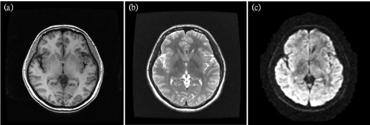
Non-invasive magnetic resonance (MR) images are extensively used in computational anatomy. Generally, MR imaging (MRI) provides good intensity contrast between soft tis-sues compared to other 3-D imaging methods, such as computed tomography (CT) and ultrasound imaging. The acquisitions of MR images with different pulse sequences result in distinct image properties which are valuable to varied clinical and research applications. For example, the majority of brain structural analyses prefer T1 weighting (Fig. 1.1a) be-cause it performs best at defining anatomy. T2-weighted scans (Fig. 1.1b) are sensitive to water content and thus are well suited to the diagnosis of edema. Increasing brain morpho-metric studies utilize diffusion tensor images (Fig. 1.1c) to investigate the abnormalities or changes of white matter (WM) because it is capable of revealing subtle fiber alterations [9]. Computational approaches established for structural analysis include voxel-based mor-phometry (VBM), deformation-based mormor-phometry (DBM), and surface-based morphom-etry (SBM) [10]. VBM differentiates anatomical differences between spatially normal-ized image groups in a voxel-wise manner [11]. Instead of the utilization of aligned brain images, DBM examines anatomical shape based on the deformation fields obtained from highly non-rigid registration [12]. SBM employs surface model to characterize the shape

Figure 1.1: MR images acquired using different pulse sequences. (a) T1-weighted MR image. (b) T2-weighted MR image. (c) Diffusion tensor image.

properties of brain anatomy [13], such as the cortical thickness [14], sulcal depth [15], and surface curvature [16]. All these morphometric methodologies heavily rely on computer-ized algorithms though they are different in the underlying theoretical frameworks.

Voxel-based structural analysis of brain MR images requires a number of image pro-cessing tasks before the statistical inference, as shown in Fig. 1.2. Due to the technical fac-tors of MRI, the intensity of homogeneous tissue is seldom uniform in each scanned image (Fig. 1.3) and may greatly alter between multi-site acquisitions (Fig. 1.4). Reducing inten-sity inhomogeneity and variability facilitates the accuracy and robustness of inteninten-sity-based image-processing algorithms as well as the reliability of structural analysis results [17,18]. Image segmentation techniques, brain extraction and tissue segmentation methods, are used to determine the regions concerned in morphometric analysis, such as specific anatomical structures or the WM, gray matter (GM), and cerebrospinal fluid (CSF) tissues. Consid-ering the accuracy of inhomogeneity correction, brain extraction is generally performed beforehand [19,20]. Image normalization spatially registers homologous anatomical struc-tures of intra- or inter- subjects to a standard stereotactic space. The standard space used in morphometric analysis is commonly defined by an average brain template which well represents the population [21] and is annotated with anatomical labels, such as the

MNI-305 [22] and MNI-152 [23]. Once brain structures are spatially aligned, image groups can be compared statistically in a voxel-wise manner.

Brain extraction Intensity correction/standardization Tissue segmentation Spatial normalization Statistical analysis Image acquisition Brain template construction MRI database T1/T2/PD/DTI Brain templates T1/T2/PD/DTI

Figure 1.2: Brain morphometric analysis system. This dissertation focuses on the develop-ment of brain extraction and brain registration techniques. The developed image-processing algorithms were used for the structural analysis of bipolar patients.

1.2

Research scope

Toward an accurate and efficient structural analysis of human brain, this dissertation fo-cuses on the development of brain extraction and brain registration techniques. The devel-oped image processing techniques were implemented in a morphometric analysis protocol for the investigation of fiber pathology between bipolar I and II disorders.

Figure 1.3: Intensity inhomogeneity of T1-weighted MR image. The right-posterior tissues highlighted in dashed boxes show obviously higher intensity compared to other regions.

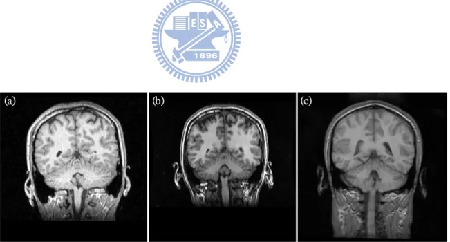
Figure 1.4: T1-weighted MR images acquired from different scanners present quite differ-ent intensity properties. MR images (a), (b), and (c) were scanned on a Bruker MedSpec S300 3T system, GE Signa EXCITE 1.5T system, and Siemens Magnetom 1.5T system, respectively.

Brain extraction from head MR image is a classification problem of segmenting im-age volumes into brain and non-brain regions. The difficulties of brain extraction primarily arise from the complicated brain surface and the varied intensity properties of images. Usu-ally intensity is utilized to differentiate between brain and non-brain tissues. However, the inevitable image artifacts, intensity inhomogeneity, inapparent brain/non-brain boundaries, and the diverse intensity profiles of multi-site images can degrade the extraction perfor-mance significantly, especially for the methods based on intensity thresholding and region clustering. Extraction algorithms using deformable models are generally more robust to both image artifacts and boundary discontinuities [24–26], but these kind of methods are commonly hard to tackle the varied curvature of brain surface [24, 27].

This thesis presents a brain extraction method which utilizes a new implicit deformable model to well represent the brain contour and to segment the brain region of MR image with high accuracy. The deformable model is described by a set of Wendland’s radial basis functions (RBFs) and has the advantages of compact support property and low computa-tional complexity. Driven by the internal force for imposing the smoothness constraint and the external force for considering the intensity contrast across boundaries, the deformable model of a brain contour can efficiently evolve from its initial state toward its target by iteratively updating the RBF locations. In the proposed method, brain contours are sepa-rately determined on 2-D coronal and sagittal slices. The results from these two views are generally complementary and are thus integrated to obtain a complete 3-D brain volume.

Registration of MR brain images is a geometric operation that determines point-wise correspondences between two brains. Convoluted brain structures and considerable data amount pose obstacles to the registration of brain images, in terms of alignment accuracy and execution efficiency. Highly non-rigid method is indispensable for the alignment of brain structures with inter-subject variance or intra-subject deformation. However, it is generally difficult to determine a good spatial mapping between brains in a large parameter space. High-resolution images are helpful for precise morphometric analysis, but the large

amount of data contributes to the major computational burden in registration process. On the other hand, the registration of low-resolution images is relatively time efficient at the expense of the degradation of alignment accuracy.

This thesis presents novel methods that can rapidly and accurately register brain images by utilizing the brain structure information estimated from image derivatives. Source and target image spaces are related by affine transformation and non-rigid deformation. The deformation field is modeled by a set of Wendland’s RBFs hierarchically deployed near the salient brain structures. In general, nonlinear optimization is heavily engaged in the parameter estimation for affine/non-rigid transformation and good initial estimates are thus essential to registration performance. In this work, the affine registration is initialized by a rigid transformation, which can robustly estimate the orientation and position differences of brain images. The parameters of the affine/non-rigid transformation are then hierarchi-cally optimized in a coarse-to-fine manner by maximizing an image similarity measure, the correlation ratio, between the involved images.

Bipolar disorder is a psychiatric illness which affects approximately 5% of the general population [28]. According to the clinical characteristics, bipolar disorders can be catego-rized into several subtypes, including bipolar I, bipolar II, cyclothymia, and bipolar disorder not otherwise specified. Although patients with bipolar I and II disorders exhibit hetero-geneous clinical presentations and cognitive functions, it remains unclear whether these two subtypes have distinct neural substrates [29–31]. This dissertation utilized fractional anisotropy maps calculated from diffusion tensor images to investigate the white matter integrity of bipolar I and II disorders in a voxel-wise manner. Diffusion tensor imaging was utilized because it is capable of detecting subtle fiber alterations [32]. The developed brain extraction and registration algorithms were adopted in this morphometric study for efficient and accurate image processing as well as reliable analysis results.

1.3

Thesis organization

The rest of this thesis is organized as follows. Chapter 2 introduces the proposed im-plicit deformable model as well as the application in brain extraction. The registration techniques presented in Chapter 3 comprise an affine and a non-rigid approaches. Chap-ter 4 introduces the morphometric analysis conducted to examine the neuropathological substrates of bipolar I and II disorders. Finally, Chapter 5 concludes the researches pre-sented in this dissertation.

2.1

Background and related works

Brain extraction is essential or beneficial to many neuroimaging applications. For ex-ample, removal of the non-brain tissues facilitates the correction of intensity non-uniformity for MR images [20]. Tissue segmentation algorithms for separating brain regions into GM, WM, and CSF usually incorporate brain extraction as a preprocessing step to simplify the segmentation problem [33–35]. Extraction of brain regions can improve the accuracy of brain image registration by avoiding the interference of inter-subject variation of non-brain structures [36], including affine and non-rigid methods [37–39]. In the past decade, VBM [11] has been extensively applied to statistically reveal regions with significant struc-tural discrepancy between image groups [1,3,40–42]. Recent studies indicated that accurate brain extraction can improve the validity of VBM results because of better tissue segmen-tation and brain registration [20,43].

Brain extraction algorithms can be classified into four major classes: (1) threshold-ing/clustering based methods, (2) boundary-based methods, (3) deformable model meth-ods, and (4) hybrid methods. Thresholding/clustering based methods extract brain regions according to the phenomenon that intensities of the voxels belonging to the same tissue are similar. Lemieux et al. proposed a fine-tuned algorithm which utilizes several inten-sity thresholds and morphological operations to remove non-brain areas [44]. Analysis of Functional NeuroImages (AFNI) fits a Gaussian mixture model to the intensity histogram of a brain image and estimates an intensity range to segment the brain areas in a slice-by-slice manner [45, 46]. Hahn and Peitgen presented a watershed algorithm which uses a connectivity criterion, pre-flooding height, to group image voxels with similar intensities and then regards the largest connected component as the brain volume [47]. More exam-ples can be found in [48–53]. Methods of this type are usually sensitive to image scanning parameters and image artifacts, such as noise and intensity inhomogeneity. Therefore, user intervention is usually required to determine proper parameters.

Boundary-based methods locate brain boundaries using the edge information obtained from image derivatives. Bomans et al. presented a semi-automated algorithm in which the brain region was manually labelled from the connected components detected with the Marr-Hildreth operator [54]. Brain Surface Extractor (BSE) method improved the work of Bomans et al. by adaptively smoothing the noisy regions, detecting structure edges, and au-tomatically determining the brain volume [35,55]. In contrast to the thresholding/clustering based approaches, these methods are less sensitive to intensity inhomogeneity and scanning parameters. However, automated methods of this type may encounter difficulties in differ-entiating true boundaries from the false ones. For example, the GM/WM edges are usually very close to the target boundaries, the CSF/GM edges, and thus may perplex the determi-nation of the brain volume.

Extraction methods using deformable models segment brain volumes by evolving con-tour or surface toward the target. Deformable model can be characterized by its repre-sentation method, implicit or explicit, and the evolution scheme [56, 57]. An explicit model directly describes the brain contour or surface and the fitting process is usually rapid [24,33,58,59]. On the other hand, implicit model can easily change the model topol-ogy, for example, to split or merge objects, but the computational complexity is usually high. The level set method adopted in Zhuang et al.’s work [26] is an example of this kind of methods. Brain extraction using deformable model is generally more robust and accu-rate compared to the thresholding/clustering based and boundary-based methods [24–26]. Moreover, incorporation of constraints or prior knowledge about the brain shape is rela-tively easy for this kind of methods. Therefore, they are more robust to both image artifacts and boundary discontinuities and can achieve subvoxel accuracy [56].

Hybrid approaches integrate the methods of different types with the anticipation to draw on the specific strengths at the expense of more computational cost [60–65]. S´egonne et al. applied the watershed algorithm [47] to generate an initial brain volume and incorporated the prior information of the brain shape into a deformable model to refine the extraction

results [25]. Rehm et al. integrated the extraction results obtained from atlas registration [36], intensity thresholding, and the BSE algorithm [35,55] by means of voting in the brain volume [66].

For large-scale studies, both accuracy and efficiency are important issues when con-sidering brain extraction algorithms [19]. The level set methods, which use implicit de-formable models, are superior in accuracy and robustness, but the computational complex-ity of these methods is usually very high. On the contrary, methods using explicit models are generally more efficient. However, the discretization process in this kind of meth-ods needs to compromise between the extraction accuracy and evolution efficiency. Finer (coarser) discretization employs more (fewer) sampling points to model object boundaries and can achieve more precise (rougher) results at a relatively slow (rapid) evolution speed. In this work, we designed a new deformable model and developed an automated brain extraction method. The deformable model is implicitly represented by a set of Wend-land’s RBFs and can efficiently evolve toward the target boundary by iterative updates of RBF locations. Because of the use of RBFs, the new model can smoothly represent object boundaries though each RBF keeps a distance to the neighboring ones. Brain contours of 2-D coronal and sagittal slices are individually fitted. The results of these two views are generally complementary and thus can be integrated to obtain accurate 3-D brain volumes. According to our experiments, the proposed brain extraction method outperformed others when jointly considering extraction accuracy and robustness.

2.2

Methods

The proposed brain extraction method comprises three major steps, as shown in Fig. 2.1. Image intensity parameters and brain centroid are first estimated for the following segmen-tation procedures. Then the proposed deformable model is applied to extract the brain area

on each of the coronal and sagittal slices. Complementary areas extracted from two dif-ferent views are then integrated into a complete 3-D brain volume. Before the detailed description of the brain extraction method, we first introduce the structure information of the brain obtained from image derivatives. The structure information is not only useful for the estimation of intensity parameters required in our brain extraction approach but for the estimation of brain orientation and the modeling of image deformation required in the proposed registration algorithms.

2.2.1

Structure information of the brain

Difference of Gaussian (DOG) performs image substraction after convolution with two Gaussian kernels 𝐺(𝜎1) and 𝐺(𝜎2), 𝜎1 > 𝜎2:

𝐷𝑂𝐺(𝐼, 𝜎1, 𝜎2) = 𝐺(𝜎1) ∗ 𝐼 − 𝐺(𝜎2) ∗ 𝐼 , (2.1)

where 𝐼 is a T1-weighted MR image and “∗” denotes the convolution operator. We define the thresholded DOG (TDOG) value to be one (foreground) when the DOG value is larger than a threshold, and otherwise the TDOG value is zero (background). Instead of using the zero-crossings of DOG results to detect edge features, we utilize the foreground in the TDOG image to reveal those regions with relatively low intensity in 𝐼, such as the GM and CSF, as shown in Fig. 2.2. We can observe that the background voxels in the brain area are mostly the WM. This information can be applied to estimate the global intensity parameters for the proposed brain extraction method. Notice that the region between two hemispheres contains mostly TDOG foreground voxels. This phenomenon can be utilized to determine the mid-sagittal planes (MSPs) and then estimate the orientation of brains. Non-brain tissues may present in TDOG foreground and can be easily removed by applying the brain masks. Then the masked foreground can guide the deployment of RBFs to cortices and ventricles in the proposed non-rigid registration method.

˖̂̅̂́˴˿ʳ̆˿˼˶˸̆ ˦˴˺˼̇̇˴˿ʳ̆˿˼˶˸̆ ˜́̇˸˺̅˴̇˼̂́ʳ̂˹ʳ˵̅˴˼́ʳ̅˸˺˼̂́̆ʳ˸̋̇̅˴˶̇˸˷ʳ˹̅̂̀ʳ˶̂̅̂́˴˿ʳ˴́˷ʳ̆˴˺˼̇̇˴˿ʳ̆˿˼˶˸̆ ˕̅˴˼́ʳ˸̋̇̅˴˶̇˼̂́ʳ̂́ʳ˶̂̅̂́˴˿ʳ˴́˷ʳ̆˴˺˼̇̇˴˿ʳ̆˿˼˶˸̆ ˘̆̇˼̀˴̇˼̂́ʳ̂˹ʳ˼̀˴˺˸ʳ˼́̇˸́̆˼̇̌ʳ̃˴̅˴̀˸̇˸̅̆ʳ˴́˷ʳ˵̅˴˼́ʳ˶˸́̇̅̂˼˷ ˼́̇˸́̆˼̇̌ ̉̂̋˸˿ʳ́̈̀˵˸̅ t2 t1t ˜́̇˸́̆˼̇̌ʳ˻˼̆̇̂˺̅˴̀ ˕̅˴˼́ʳ˶˸́̇̅̂˼˷ʳ˿̂˶˴˿˼̍˴̇˼̂́ ˘̆̇˼̀˴̇˼̂́ʳ̂˹ʳ˺˿̂˵˴˿ʳ˖˦˙ʳ˼́̇˸́̆˼̇̌ʳ̇˶ ˘̆̇˼̀˴̇˼̂́ʳ̂˹ʳ˺˿̂˵˴˿ʳ˪ˠʳ˼́̇˸́̆˼̇̌ʳ̇̊ ʻ˴ʼ ʻ˵ʼ ʻ˶ʼ ʻ˷ʼ ʻ˸ʼ ʻ˹ʼ

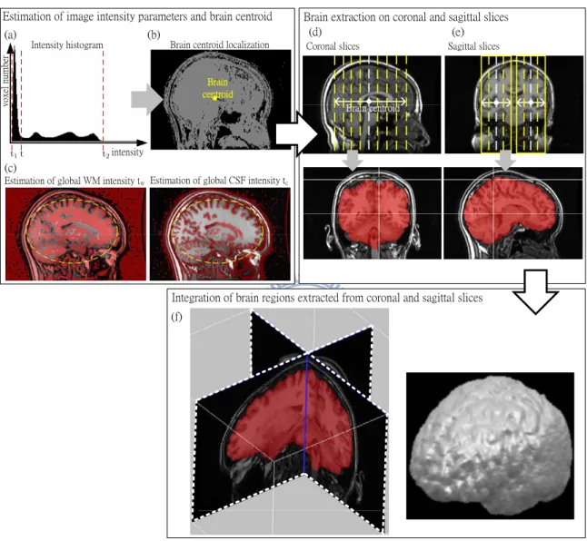
Figure 2.1: Flowchart of the brain extraction method. (a) The effective intensity range [𝑡1, 𝑡2] and a rough head/background threshold 𝑡 are estimated from the intensity histogram.

(b) Then the voxels with intensity value within [𝑡, 𝑡2] are used to approximate the brain

centroid. (c) Applying DOG operator with zero threshold, the global WM intensity 𝑡w and

CSF intensity 𝑡care decided from the voxels within the ellipsoid approximating the brain

shape. The brain areas of the (d) coronal slices and (e) sagittal slices are extracted. (f) A complete 3-D brain region is determined from the complementary areas segmented from two different views.

L (a) (b) X (c) (d) (e) X

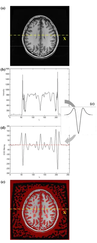
Figure 2.2: The TDOG foreground reveals the regions with relatively low intensities. (a) One axial slice of a T1-weighted MR brain image. (b) The pixel intensity profile on the scan line X. (c) An example of DOG kernel. (d) The results obtained by convolving DOG kernel to the scan line X. (e) Image overlay of the the 2D TDOG foreground (in red color) on the axial slice.

2.2.2

Estimation of image intensity parameters and brain centroid

intensi-ties, such as noises or DC spikes, in which 𝑡1and 𝑡2are the intensity values in the histogram

such that the accumulated number of voxels reaches 2% and 98%, respectively, as shown in Fig. 2.1. To roughly separate the head from the background, the threshold 𝑡 is set to be 10% in the range of [𝑡1, 𝑡2]. The brain centroid O is calculated by the first order image moment

using the voxels with intensity value in the range of [𝑡, 𝑡2].

An ellipsoid approximating the brain shape is determined by detecting the head bound-ing box from those voxels with intensity within [𝑡, 𝑡2]. The polar radius is set to the distance

between the centroid and superior plane and the two equatorial radii are set to the halves of the distances between the opposite bounding planes, that is, the left-right and the anterior-posterior planes.

The voxels with DOG values smaller than zero are in the regions with relatively high intensities, which are mostly the WM areas in the brain. Therefore, the median intensity of these voxels within the brain-approximating ellipsoid estimates the global WM intensity, 𝑡w. On the other hand, the regions with DOG values larger than zero indicate the tissues

with relatively low intensities. These voxels within the ellipsoid are mostly the GM and CSF. We apply Otsu’s algorithm [67] to calculate an intensity threshold 𝑡o for separating

CSF voxels from GM voxels. The median intensity of the CSF voxels estimates the global CSF intensity, 𝑡c.

2.2.3

Brain extraction on the slices in two views

Brain extraction using deformable model generally requires a constraint to keep the contour or surface smooth. Loosening this constraint may lead to better fitting for the

uneven brain surface but may face the risk of leakage through the weak boundaries. On the other hand, models with strict smoothness constraint can achieve stable results, but they usually underestimate the curvature of brain surface. To tackle this problem, Smith utilized a hyperbolic tangent function with empirically obtained maximum and minimum curvature values to adaptively smooth the model of brain surface [24].

In this work, we apply the deformable contour model to extract the brain regions on both coronal and sagittal slices and then integrate the results from two views. As shown in Fig. 2.3, local curvatures of a region extracted from different views are usually quite different. Fitting a local boundary in the view with relatively low curvatures often achieve more reliable results, whereas the boundaries frequently cut through the tissues due to the high curvatures in another view. Therefore, segmentation results in different views can complement each other. Applying a strict smoothness constraint for two views followed by the simple logical OR operation for the integration can achieve accurate and stable extraction. Notice that brain extraction on the axial slices is not considered in this work because of the efficiency issue.

The segmentation in the coronal view starts with the slice nearest to the brain centroid

O and proceeds with the slices toward the anterior and posterior directions. The extraction

on the sagittal slices, which are parallel to the detected MSP, is divided into two parts. Each part starts with a sagittal slice 30 mm apart from the MSP and proceeds with the slices toward the MSP and the most lateral slice, as shown in Fig. 2.1. Sagittal slices within 3 mm from the MSP are not processed to avoid the unstable segmentation due to relatively few GM and WM tissues. Because the extracted brain region shrinks gradually as the extraction goes forward along the anterior, posterior, left, and right directions, brain extraction in each of these directions is terminated once the size of the extracted brain region is smaller than a threshold.

ʻ˴ʼ ʻ˵ʼ ʻ˶ʼ _{ˣ˿˴́˸ʳ˅} ˣ˿˴́˸ʳ˄ ̆̈̅˹˴˶˸ ˶̂́̇̂̈̅ʳ˼́ʳˣ˿˴́˸˅ ˶̂́̇̂̈̅ʳ˼́ʳˣ˿˴́˸˄

Figure 2.3: Brain surface presents quite different curvatures in the coronal and sagittal views. (a) The yellow curves show that the local curvature of brain surface in the coronal view is significantly higher than that in the sagittal view, and (b) vice versa. (c) Boundary fitting can achieve more reliable results with low curvatures than with high curvatures. The regions marked as red in (a) and (b) illustrate that the fitting results obtained from coronal and sagittal views are mutually complementary.

Figure 2.4: Initial brain contour. An elliptic contour centered in the approximated bounding box of the brain is regarded as the initial contour for the brain extraction on each of the starting slices.

2.2.4

Initial contour

An initial contour within the brain region is required for each of the three starting slices, as shown in Fig. 2.4. The brain bounding box is first detected from those pixels with their intensity values within [𝑡, 𝑡2]. In this way the lower boundary of the bounding box is usually

located at the bottom of the MR volume and is thus adjusted according to the aspect ratios 8:7 and 4:3 for the coronal and sagittal slices, respectively. A set of Wendland’s RBFs are then equally spread along an ellipse centered in the bounding box with the lengths of its axes set to be 0.7 times the length and width of the box. These RBFs determine an initial contour which can evolve to fit the brain contour by the method described in the next section. Because the brain contours of adjacent slices are usually similar, the evolved contour of current slice provides a good initial for the neighboring ones. This propagation way improves the performance of brain extraction, in terms of both accuracy and efficiency.

2.2.5

Deformable model for brain extraction

A contour in a 𝑑-dimensional image space (𝑑 is 2 or 3) can be implicitly modeled as the zero set of a scalar function 𝜑 : ℜ𝑑 _{→ ℜ:}

𝐶 = {x ∣ 𝜑(x) = 0, x ∈ ℜ𝑑_{} . (2.2)}

In this work, we define the scalar function 𝜑(⋅) as the sum of 𝐾 weighted RBFs:

𝜑(x) = ∑𝐾

𝑖=1

𝑇𝑖(x − c𝑖)𝜙𝑠(∥x − c𝑖∥) , (2.3)

where ∥ ⋅ ∥ is the Euclidean norm and 𝑇𝑖(⋅) is a weighting function for the RBF 𝜙𝑠(⋅). The one-argument function 𝜙𝑠: ℜ+ → ℜ is the RBF centered at c𝑖, c𝑖 ∈ ℜ𝑑. This work adopts

the Wendland’s 𝜓-functions, 𝜓3,1, as the function 𝜙𝑠because of its advantages of compact support property and low computational complexity [68, 69]:

𝜙𝑠(𝑟) = ⎧ ⎨ ⎩ (1 − 𝑟 𝑠)4(4𝑟𝑠 + 1) , 0 ≤ 𝑟 < 𝑠 0 , 𝑠 ≤ 𝑟 , (2.4)

where 𝑠 is the shape parameter for accommodating various extents of the compact support. Given the outward normal vector n𝑖 at c𝑖, the weighting function 𝑇𝑖 : ℜ𝑑 → ℜ is defined as:

𝑇𝑖(v) = v𝑡n𝑖 . (2.5)

Therefore, each 𝑇𝑖(⋅)𝜙𝑠(⋅) term in Eq. (2.3) implicitly represents a line as the zero set in 2D image space. The normal vector at the RBF center determines the orientation of the line and the summation of these products results in a smooth contour representation, as illustrated in Fig. 2.5. Notice that we only consider the zero set within the support extents of RBFs and usually the contour does not pass through RBF centers in this model. From the implicit function, the normal vector n𝑖 at the control point c𝑖 is calculated as

ʻ˴ʼ ʻ˵ʼ ˀ˄ˋ ˄ˉ ˀ˄ˋ ˄ˉ ˀ˅ˌ ˄ˊ T1(x ¡ c1)Ás(kx ¡ c1k) = 0 T1(x ¡ c1) = (x¡ c 1)tn1 x ¡ c1 x c1 n1 T2(x ¡ c2)Ás(kx ¡ c2k) = 0 '(x) = 2 X i=1 Ti(x ¡ ci)Ás(kx ¡ cik) = 0 n1 n2 x T1(x ¡ c1) T2(x ¡ c2) n2 c2 c2 c1

Figure 2.5: Implicit contour representation. (a) Image intensity in this figure represents the value of 𝑇𝑖(⋅)𝜙𝑠(⋅). The zero set where 𝑇𝑖(⋅)𝜙𝑠(⋅) = 0 within the compact support region represents the implicit model, marked as the red line. (b) The combination of 𝑇𝑖(⋅)𝜙𝑠(⋅) can represent contour smoothly.

During the contour evolution, we adaptively allocate or deallocate RBFs according to the distance between the neighboring RBF centers.

Contour evolution forces

The brain area on each slice is determined by iteratively moving each RBF center c𝑖 along the normal direction n𝑖 to a compromise between an internal force 𝐹s(c𝑖) and an

external force 𝐹e(c𝑖), 𝑖 = 1 . . . 𝐾:

∂c𝑖

∂𝑡 = (𝑎𝐹s(c𝑖) + 𝑏𝐹e(c𝑖)) n𝑖 , (2.7)

where the weighting parameters 𝑎 and 𝑏 are both generally set to be 0.5.

The internal force calculated from the contour itself is used to keep the contour smooth during the evolution process. We define the smoothness constraint function 𝐹s(⋅) at c𝑖 as

normal vectors n𝑖−1and n𝑖+1of c𝑖’s neighboring RBFs centered at c𝑖−1and c𝑖+1:

𝐹s(c𝑖) = u𝑡𝑖n𝑖× ∥n𝑖− n𝑖−1∥ + ∥n₂ 𝑖− n𝑖+1∥ , (2.8) where u𝑖is the normalized vector which starts from c𝑖 and points to the midpoint between

c𝑖−1 and c𝑖+1. Because each RBF keeps a distance to its neighboring ones, the contour smoothness is estimated from a larger scale of view, compared to the local curvature ∇n𝑖 estimated at c𝑖.

The external force is used to evolve the initial contour toward its target boundary. Here we modify the external force adopted in Zhuang et al.’s work [26], which originated from [33] and [24], as follows:

𝐹e(c𝑖) = 𝑤(𝑑, 𝛼, 𝑠′) × (_𝐼𝐼min(c𝑖)

max(c𝑖)− 𝛽) . (2.9)

The function above is designed according to the phenomenon that the intensity contrast between the CSF and GM/WM is usually high. Functions 𝐼min(⋅) and 𝐼max(⋅) find the

local minimum intensity and local maximum intensity, respectively, among several sampled pixels starting from each RBF center c𝑖along the opposite direction of n𝑖:

𝐼min(c𝑖) = max(𝑡1, min(𝑡m, 𝐼(c𝑖), 𝐼(c𝑖− n𝑖), 𝐼(c𝑖− 2n𝑖), . . . , 𝐼(c𝑖− 𝑀n𝑖))) , (2.10)

𝐼max(c𝑖) = min(𝑡2, max(𝑡w, 𝑡m, 𝐼(c𝑖), 𝐼(c𝑖− n𝑖), 𝐼(c𝑖− 2n𝑖), . . . , 𝐼(c𝑖− 𝑁n𝑖))) , (2.11)

where 𝑀 and 𝑁 determine the search ranges and 𝑡mis the median intensity of the brain

tissues on each slice, which is approximated from the pixels within the initial brain region. The parameter 𝛽 is used to characterize the intensity contrast between the brain and non-brain tissues. Its value is slightly larger than the intensity ratio of the CSF to WM:

𝛽 = _𝑡𝑡c

w + 𝑘 , (2.12)

where 𝑘 is a small positive number. In this way the value of the parameter 𝛽 is not fixed but adaptively determined because the WM and CSF intensities, 𝑡w and 𝑡c, are estimated from

method. Generally, the distance 𝑁 in 𝐼max(⋅) should be large enough to reach the WM

during the evolution. Therefore, 𝐼max(⋅) roughly equals to the local WM intensity. If the

evolving contour is inside the brain region, 𝐼min(⋅) is most likely the intensity of GM or

WM. This results in a positive external force and drives the contour outward. Once the contour is outside the brain boundary, 𝐼min(⋅) is most likely the CSF intensity and the

resulted negative external force (approximately −𝑘) pulls the contour inward.

Because the brain boundaries of neighboring slices are usually similar, we apply a weighting function 𝑤(⋅) to constrain the moving distance 𝑑 of the RBF while the formable model evolves from its initial position. Here the weighting function 𝑤(⋅) is de-fined as the Wendland’s RBF in Eq. (2.4) with support extent 𝑠′_:

𝑤(𝑑, 𝛼, 𝑠′_{) = 𝜙𝑠′(max(0, 𝑑 − 𝛼)) . (2.13)}

As the example shown in Fig. 2.6, 𝑤(⋅) begins to gradually decrease to zero when the moving distance 𝑑 is larger than 𝛼. Therefore, this function regularizes the amount of brain contour evolution and thus imposes the smoothness constraint of the extracted brain volume across adjacent slices. Note that this term is set to be the constant one in the extraction process for each of the starting slices.

2.2.6

Integration of segmentation results

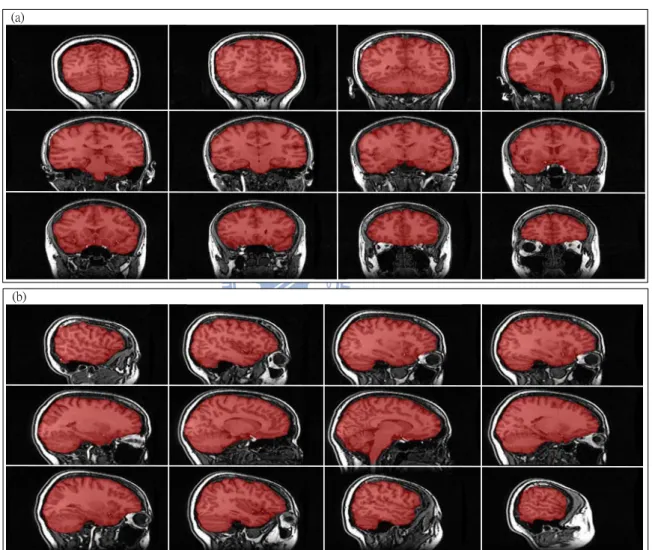
The brain regions determined from the coronal and sagittal slices are complementary and thus can be integrated to increase the sensitivity of brain extraction. Segmentation results of the sagittal slices are first transformed back to the native space because these slices are sampled from the planes parallel to the detected MSP. Logical OR operation is then applied to combine the coronal and the transformed sagittal results. Finally, we apply morphological opening with a circle as the structural element to remove the weak connected components and to smooth the brain surface. Fig. 2.7 illustrates the extraction results of a T1-weighted head image.

0 2 4 6 8 10 0 0.2 0.4 0.6 0.8 1 d w(d, α ,s’)

Figure 2.6: The weighting function 𝑤(𝑑, 𝛼, 𝑠′_{) used to constrain the moving distance 𝑑 of} the RBF while evolving from its initial position. In this example, 𝛼 and 𝑠′ _{are set to be 2} and 5, respectively.

2.2.7

Performance evaluation

This section introduces the methods used to evaluate the performance of the proposed brain extraction algorithm, including the data sets, performance criteria, and the approaches used for comparisons. The obtained accuracy evaluation results are further analyzed by two-sample t-test for performance comparison among the brain extraction methods. More-over, previous evaluation works can be found in [19, 70, 71].

Brain extraction algorithms for performance comparisons

The proposed method was compared with the Brain Surface Extractor (BSE) in Brain-Suite2 [35,55,72], Brain Extraction Tool (BET) version 2.1 [24,73], Hybrid Watershed Al-gorithm (HWA) version stable 3 [25], and Model-based Level Set (MLS) version 0.5 [26]. The programs of the compared methods used in our experiments were downloaded from their webpages. BET, BSE, HWA, and our method were implemented in C++ whereas MLS was programmed in Java. All extraction experiments were performed on an AMD

ʻ˴ʼ

ʻ˵ʼ

Figure 2.7: Brain extraction results of a T1-weighted image shown in (a) coronal and (b) sagittal views.

Opteron 240 processor running Linux, except BSE. Software of BSE is available only for Windows system, thus we evaluated its performance on another machine with an AMD XP 2400+ processor. Furthermore, we adopted the nearest neighbor sampling in our imple-mentation not only because of its efficiency but also its accuracy compared to the trilinear interpolation. This observation agrees with the findings in [24]. The reason could be that sampling methods other than the nearest neighbor somewhat blur images and the resulted weak boundaries may deteriorate the accuracy of brain extraction.

Image data sets with manual segmentation results

Two sets of T1-weighted head MR images as well as manual segmentation results were obtained from the Internet Brain Segmentation Repository (IBSR)1_{. In the experiments,}

we applied extraction algorithms to determine the brain volumes of these subjects and employed the manually segmented brain areas, including the ventricles, to evaluate the extraction accuracy.

The first IBSR data set comprises twenty MR volumes, each with around 60 coronal slices, matrix size 256 × 256, FOV 256 × 256 mm2_{, and slice thickness 3.1 mm. Obvious}

intensity inhomogeneity and other significant artifacts present in most of the MR images in this data set. Another challenge of this data set is that the neck and even shoulder areas are included. This may influence the extraction accuracy of BET and HWA methods, as the examples shown in Figs. 2.8a and 2.8c (HWA even failed to process eighteen of the twenty MR images), because the excess non-brain tissues severely bias the estimation of the required parameters. To fairly evaluate extraction performance, several inferior slices of the image volumes containing neck or shoulder area were manually removed beforehand. In this way, BET and HWA achieved better segmentation results, as shown in Figs. 2.8b and 2.8d.

1_{IBSR was developed by the Center for Morphometric Analysis at Massachusetts General Hospital and is}

The second IBSR data set contains eighteen MR images, each with around 128 coronal slices, matrix size 256 × 256, FOV 240 × 240 mm2_{, and slice thickness 1.5 mm. All}

images were transformed to radiological convention beforehand based on the orientation information obtained from IBSR. These images have superior quality in contrast to those in the first data set. According to the document of IBSR, each image in this data set has been roughly registered to the Talairach space and the intensity inhomogeneity has been corrected using the software developed by the Center for Morphometric Analysis at the Massachusetts General Hospital.

Criteria for extraction accuracy assessment

Several criteria are utilized to measure the extraction accuracy, including the Jaccard similarity coefficient (JSC), the sensitivity and specificity coefficients, and the risk evalua-tion of the segmentaevalua-tion results. The JSC, also known as the Jaccard index, is an extensively adopted measurement which evaluates the similarity between the extracted brain region 𝐵 and the corresponding ground truth 𝐴:

𝐽𝑆𝐶(𝐴 , 𝐵) = ∣𝐴 ∩ 𝐵∣

∣𝐴 ∪ 𝐵∣ , (2.14)

where ∣ ⋅ ∣ denotes the cardinality value. The value of JSC is within [0, 1] and a larger JSC value means a better overlap with the ground truth.

Brain extraction is usually a compromise between the high recognizing percentage for brain voxels (that is, high sensitivity) and the high rejecting percentage for non-brain voxels (that is, high specificity). Therefore, the coefficients of sensitivity 𝑆eand specificity 𝑆pcan

be used to characterize brain extraction algorithms:

𝑆e= _{TP + FN}TP , (2.15)

The true positive rate, TP, and false positive rate, FP, are the number of voxels correctly and incorrectly classified as brain tissues, respectively. The true negative rate, TN, and false negative rate, FN, are the number of voxels correctly and incorrectly classified as non-brain tissues, respectively.

In some applications, it is more important to avoid missing brain tissues than to reject all non-brain regions. From this point of view, S´egonne et al. proposed an error function 𝐸 to measure the extraction risk [25]:

𝐸(𝑐) = 𝑝f_{1 + 𝑐}+ 𝑐𝑝m , (2.17)

where 𝑐 is the risk ratio between the probabilities of missed detection for brain tissues, 𝑝m,

and false alarm, 𝑝f. These two probabilities are calculated as

𝑝m = ∣𝐴 − 𝐵∣_{∣𝐴 ∪ 𝐵∣} , (2.18)

𝑝f = ∣𝐵 − 𝐴∣_{∣𝐴 ∪ 𝐵∣} , (2.19)

where 𝐵 is the extracted brain region, 𝐴 is the corresponding ground truth, and ∣ ⋅ ∣ denotes the cardinality value.

Parameters of brain extraction algorithms

The parameters of the compared methods were determined to achieve the best average JSC value for each data set. In other words, there were two sets of parameter values for each method and each set is for one data set. For the first (second) IBSR image set, the smoothness weighting of MLS was chosen as 0.05 (0.1); the fractional intensity threshold of BET was set to be 0.6 (0.7); the parameters of HWA were set to the default values (default values with surface-shrink option turned on); the parameter 𝑘 of the proposed method was set to be 0.15 (0.15); and the edge constant, diffusion iteration, and diffusion constant of BSE were set to be 3 (3), 1 (1), and 0.70 (0.66), respectively.

2.3

Experimental results

This section presents our results of performance evaluation for brain extraction meth-ods. Table 2.1 lists the experimental outcomes of the proposed and other brain extraction algorithms using the first IBSR data set. In general, MLS and our method performed better than others. Jointly considering both the sensitivity and specificity, the accuracy indices of BET and BSE were moderate among the five methods evaluated. In this experiment, HWA did not achieve significant outperformance for all accuracy criteria (𝑝 > 0.05). Notice that the performance indices of each method shown in Table 2.1 did not count in the cases that (1) the JSC value between the extracted brain volume and the ground truth is smaller than 0.6 (three cases for BSE); (2) the program terminates without any results (three cases for HWA); and (3) the extraction result is blank (one case for BSE and one case for MLS). Ex-cluding these cases (seven in total), all methods achieved slightly larger JSC values, which means better overlapping of the extracted brain regions with the ground truths, as shown in Table 2.2. HWA had remarkable improvement in its sensitivity due to the omission of additional four poor cases. Because of the exclusion of these seven cases, outperformance of BSE and MLS to our method became significant in terms of the specificity (𝑝 = 0.001) and JSC (𝑝 = 0.024), respectively.

To verify that the manual removal of slices containing neck or shoulder region in the first experiment did not largely affect the performance for BSE, MLS, and the proposed methods, we applied these three algorithms again to extract the brain volumes from original IBSR images. The obtained results indicated that these three algorithms produced similar extraction outcomes no matter the excess non-brain slices were removed or not.

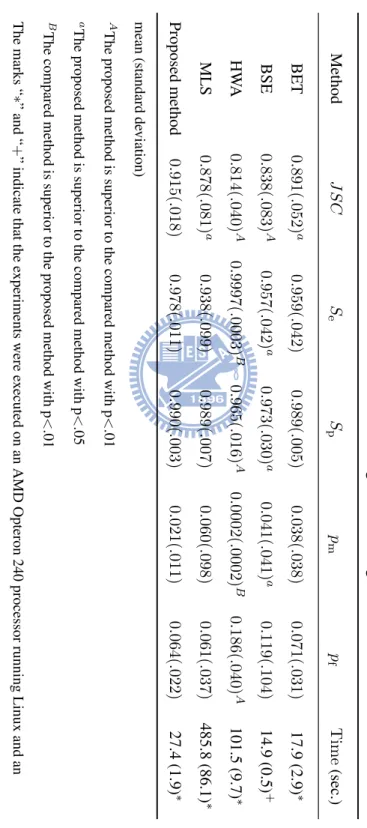
Table 2.3 lists the experimental results of the proposed and other extraction algorithms using the second IBSR data set. Our method generally performed better than others with respect to all accuracy criteria, except for the sensitivity. HWA achieved the best sensitivity in detecting brain tissues at the expense of the relatively low specificity. BET, MLS, and

ʻ˴ʼ ʻ˵ʼ ʻ˶ʼ ʻ˷ʼ ˕˘˧ ˢ̈̅ʳ̀˸̇˻̂˷ ˢ̈̅ʳ̀˸̇˻̂˷ ˛˪˔ ˢ̈̅ʳ̀˸̇˻̂˷ ˛˪˔ ˢ̈̅ʳ̀˸̇˻̂˷ ˕˘˧

Figure 2.8: Excess non-brain tissues affect the extraction accuracy of BET and HWA. The MR images of the first IBSR data set contain neck areas, as shown in the left of (a) and (c). In this case BET and HWA cannot well extract the brain volumes, as shown in the middle of (a) and (c). Manually removing several inferior non-brain slices, as shown in the left of (b) and (d), can facilitate BET and HWA to produce better extraction results, as shown in the middle of (b) and (d). On the other hand, the proposed method is relatively robust to the excess non-brain tissues, as shown in the right from (a) to (d).

Table 2.1: Performance ev aluation using the first IBSR data set after excluding the unsatisf actory results of each brain extraction algorithm. Method 𝐽𝑆 𝐶 𝑆e 𝑆p 𝑝m 𝑝f Time (sec.) BET 0. 878( .017) 𝐴 0. 983( .023) 0. 987( .004) 𝑎 0. 016( .022) 0. 107( .021) 𝐴 11.4 (.8) ∗ BSE 4 0. 900( .025) 0. 954( .035) 𝐴 0. 993( .003) 0. 044( .034) 𝐴 0. 055( .017) 𝐵 3.6 (1.0) + HW A 3 0. 752( .037) 𝐴 0. 974( .068) 0. 970( .008) 𝐴 0. 022( .056) 0. 226( .026) 𝐴 96.1 (24.7) ∗ MLS 1 0. 922( .025) 0. 989( .010) 0. 992( .006) 0. 011( .009) 0. 067( .031) 228.6 (28.0) ∗ Proposed method 0. 910( .018) 0. 986( .013) 0. 991( .005) 0. 013( .013) 0. 077( .027) 14.4 (3.6) ∗ mean (standard de viation) 𝐴 The proposed method is superior to the compared method with p< .01 𝑎The proposed method is superior to the compared method with p< .05 𝐵 The compared method is superior to the proposed method with p< .01 The superscripts in the first column indicate the number of the excluded cases. The marks “∗ ” and “+ ” indicate that the experiments were ex ecuted on an AMD Opteron 240 processor running Linux and an AMD XP 2400+ processor running W indo ws XP ,respecti vely .

Table 2.2: Performance ev aluation using the first IBSR data set without considering all the cases which caused unsatisf actory results. Method 𝐽𝑆 𝐶 𝑆 e 𝑆 p 𝑝 m 𝑝 f Time (sec.) BET 7 0.881( .017) 𝐴 0.981( .026) 0.988( .003) 𝐴 0.017( .024) 0.102( .021) 𝐴 11.5 (.9) ∗ BSE 7 0.905( .025) 0.954( .035) 𝐴 0.994( .002) 𝐵 0.044( .034) 𝐴 0.051( .010) 𝐵 3.7 (1.0) + HW A 7 0.762( .012) 𝐴 0.999( .001) 𝑏 0.967( .008) 𝐴 0.001( .001) 𝑏 0.237( .013) 𝐴 91.6 (16.2) ∗ MLS 7 0.922( .023) 𝑏 0.989( .010) 0.992( .006) 0.011( .010) 0.067( .030) 𝑏 230.2 (30.0) ∗ Proposed method 7 0.911( .014) 0.988( .015) 0.991( .004) 0.012( .014) 0.077( .023) 19.9 (2.9) ∗ mean (standard de viation) 𝐴 The proposed method is superior to the compared method with p< .01 𝑎 The proposed method is superior to the compared method with p< .05 𝐵 The compared method is superior to the proposed method with p< .01 𝑏 The compared method is superior to the proposed method with p< .05 The superscripts in the first column indicate the number of the excluded cases. The marks “∗ ” and “+ ” indicate that the experiments were ex ecuted on an AMD Opteron 240 processor running Linux and an AMD XP 2400+ processor running W indo ws XP ,respecti vely .

BSE were statistically equal in all accuracy criteria, except for the specificity of BSE. BSE had the significantly lower specificity in detecting non-brain regions compared to BET (p=0.046) and MLS (p=0.02).

Tables 2.1 to 2.3 also list the average execution time of extraction methods using the first and second IBSR data sets. Both experiments show that BSE achieved the best effi-ciency, followed by BET and our method, though BSE was executed on a relatively low-end processor. The processing time of HWA and MLS was apparently longer among the com-pared methods. Notice that MLS has a chance to achieve better efficiency if the algorithm is implemented in C/C++, instead of Java.

For each brain extraction method, the probabilities of the false classification for brain and non-brain voxels, 𝑝m and 𝑝f, were calculated to evaluate its extraction risk. Fig. 2.9a

shows the risk profiles of the first experiment when the risk ratio 𝑐 between 𝑝mand 𝑝franged

from 1 to 10. It is apparent that MLS and our method have relatively lower extraction risks. BET and HWA perform better than BSE when the risk ratio is larger than 1.8 and 8.0, respectively. This figure also illustrates the extraction risk for the results excluding the seven subjects that caused markedly poor results. We can see that the performance of the proposed method, BSE, and MLS has been slightly improved. The extraction risk of HWA decreases rapidly due to its high sensitivity to the inclusion of brain tissues. The risk profiles of the second experiment shown in Fig. 2.9b indicate that the proposed method has the lowest extraction risk compared to other algorithms if the penalty is smaller than 6. HWA performs better than BSE, MLS, BET, and our method if the risk ratio is larger than 1.6, 2.0, 3.0, and 6.0, respectively.

Table 2.3: Performance ev aluation for brain extraction algorithms using the second IBSR data set. Method 𝐽𝑆 𝐶 𝑆 e 𝑆 p 𝑝 m 𝑝 f Time (sec.) BET 0.891( .052) 𝑎 0.959( .042) 0.989( .005) 0.038( .038) 0.071( .031) 17.9 (2.9) ∗ BSE 0.838( .083) 𝐴 0.957( .042) 𝑎 0.973( .030) 𝑎 0.041( .041) 𝑎 0.119( .104) 14.9 (0.5) + HW A 0.814( .040) 𝐴 0.9997( .0003) 𝐵 0.965( .016) 𝐴 0.0002( .0002) 𝐵 0.186( .040) 𝐴 101.5 (9.7) ∗ MLS 0.878( .081) 𝑎 0.938( .099) 0.989( .007) 0.060( .098) 0.061( .037) 485.8 (86.1) ∗ Proposed method 0.915( .018) 0.978( .011) 0.990( .003) 0.021( .011) 0.064( .022) 27.4 (1.9) ∗ mean (standard de viation) 𝐴 The proposed method is superior to the compared method with p< .01 𝑎 The proposed method is superior to the compared method with p< .05 𝐵 The compared method is superior to the proposed method with p< .01 The marks “∗ ” and “+ ” indicate that the experiments were ex ecuted on an AMD Opteron 240 processor running Linux and an AMD XP 2400+ processor running W indo ws XP ,respecti vely .

ʻ˴ʼ

ʻ˵ʼ

Figure 2.9: Extraction risk evaluation using (a) the first IBSR data set and (b) the second IBSR data set. The mark “∗” indicates that some failed or extremely poor segmentation case(s) are not included. After excluding all of these cases for each method, the risk profiles are shown as the dashed lines in (a).