比較傳統與簡化的傳送器用來產生歸零-差分四元相位移鍵/振幅移鍵

國 立 交 通 大 學

光 電 工 程 研 究 所

碩士論文

比較傳統與簡化的傳送器用來產生歸零-差分四

元相位移鍵/振幅移鍵

標籤信號的效能評估

Performance evaluation of an RZ-DQPSK/ASK

label signal generated by a simple and conventional

transmitter

研

究

生 : 蔡 昇 祐

指 導 教 授 : 陳 智 弘 老師

比較傳統與簡化的傳送器用來產生歸零-差分四

元相位移鍵/振幅移鍵

標籤信號的效能評估

Performance evaluation of an RZ-DQPSK/ASK

label signal generated by a simple and conventional

transmitter

研 究 生 :蔡昇祐

Student :

Shen-You

Tsai

指導教授 :陳智弘 老師

Advisor : Assistant Prof. Jyehong Chen

國 立 交 通 大 學

光 電 工 程 研 究 所

碩 士 論 文

A Thesis

Submitted to Institute of Electro-Optical Engineering

College of Electrical Engineering and Computer Science

National Chiao Tung University

In Partial Fulfillment of the Requirements

For the Degree of

Master

In

Institute of Electro-Optical Engineering

July 2006

Hsinchu, Taiwan, Republic of China

致謝

A

CKNOWLEDGEMENTS 一轉眼兩年的碩士生涯終於要劃上句點了，很感謝在許多人的幫忙和協助才 能完成這篇碩士論文。 首先要感謝我的指導教授陳智弘老師帶領我進入光通訊這個博大森淵的領 域，使我對光通訊有了初步的了解，同時在他亦師亦友的教導下，也學習到很多 待人接物和求學應有的態度，讓我渡過愉快的兩年碩士生涯。另外特別要感謝彭 煒仁學長的指導才能使我完成這篇碩士論文，在他細心和不厭其煩的教導，以及 實驗期間他不斷容忍我所犯的過錯給我鼓勵，如果沒有彭煒仁學長的耐心指導相 信今天這篇論文無法順利誕生。還有魏嘉健學長無論是在學業及論文的研究上也 給了我許多的幫助，常常很多遇到的難題在請教他之後都能迎刃而解。 同時還有許許多多陪伴我一起渡過這難忘的兩年碩士生涯，像是之前畢業的 學長重佑、小強和小鐵跟著他們一起運動一起吃飯每天在實驗室都很愉快的渡 過，或著陪伴著我一起修課的同學小雨、鐘响和人豪能夠互相討論課業和一同實 驗，以及五樓的其他學長們都是陪伴我渡過短暫難忘的兩年碩士生涯，真的很感 謝大家。 最後要感謝我父親和母親從小栽培我支持我，讓我無後顧之憂的完成學業。 要感謝的人實在太多，總之，感謝大家。

比較傳統與簡化的傳送器用來產生歸零-差分四元相位移鍵/振幅移鍵

標籤信號的效能評估

學生：蔡昇祐 指導教授 : 陳智弘 老師

國立交通大學光電工程研究所碩士班

摘要

多重層次的調變如差分四元相位移鍵重新引起注意是因為他可增進頻譜效 率在光纖通訊系統上◦ 在這篇論文中我們提供一種簡單而且價格縮減的方式來產生歸零-差分四元 相位移鍵/振幅移鍵標籤信號，只需要兩個雙重驅動 Mach-Zehnder 調變器就可以 完成◦首先我們將第一個雙重驅動 Mach-Zehnder 調變器偏壓位置在 Vπ/2 及驅動訊 號大小 Vπ如此可用來取代兩個調變器所產生的歸零-差分四元相位移鍵，再來我 們使用混和器來混合正弦波與低速率的標籤信號再將混和後的訊號載入第二個 雙重驅動 Mach-Zehnder 調變器如此可用來取代波形切割器與振幅移鍵調變器◦最 後本論文會比較傳統歸零-差分四元相位移鍵/振幅移鍵標籤信號傳送器及簡化歸 零-差分四元相位移鍵/振幅移鍵標籤信號傳送器的效能◦

Performance evaluation of an

RZ-DQPSK/ASK label signal generated by

a simple and conventional transmitters

Student：Shen-You Tsai Advisor : Dr. Jyehong Chen

Institute of Electro-Optical Engineering

National Chiao Tung University

Abstract

Multilevel modulation signals like differential quadrature phase-shift keying (DQPSK) have received renewed attention to improve the spectral efficiency of a lightwave communication system.

In this thesis, we provide a simple and cost effective method to generate DQPSK payload/ASK label signal which only needs two dual-drive Mach-Zehnder modulator (DD-MZM). First, we use bias position (bias=Vπ/2) and drive signal of dual-drive Mach-Zehnder modulator to generated DQPSK signal which replaced two Mach-Zehnder modulator. Second, we also used mixer to mix the sinwave and the low bit rate label data into Mach-Zehnder modulator replace pulse carver and ASK modulator. Finally, the thesis evaluate performance of conventional DQPSK/ASK label transmitter and dual-drive DQPSK/ASK label signal transmitter.

C

ONTENTS

Acknowledgements

... i

Chinese Abstract

... ii

English Abstract

... iii

Contents

... iv

List of Figures

... vi

List of Tables

... ix

CHAPTER 1

Introduction

1.1 Motivation...1

1.2 Label swapping application for packet switch network…...2

1.3 New scheme to generate DQPSK payload/ASK label signal………..3

CHAPTER 2

DQPSK payload/ASK label signal

2.1 Mach-Zehnder modulator……..………...4

2.2 Differential quadrature phase shift keying (DQPSK)...5

2.2.1Convention optical DQPSK transmitter ...………….7

2.2.2 Variety of dual-drive DQPSK signals...8

2.2.3 Two level drive DQPSK transmitter...10

2.2.4 Transition of two level drive DQPSK…...12

2.2.5 Eye spreading of two level drive DQPSK………...15

2.3 Pulse carver for RZ-DQPSK……….………..………...16

2.4 DQPSK demodulation………...18

2.5 Structure of DQPSK/ASK label...20

2.5.1 Simple RZ-DQPSK/ASK Label transmitter……….………...22

CHAPTER 3

Experiment setup and result (DQPSK)

3.1 Dual-Drive DQPSK experiment setup………...23

3.3 Sensitivity of Dual-drive DQPSK…...26

3.3.1 DD NRZ DQPSK…...26

3.3.2 DD 33%RZ DQPSK...27

3.3.3 DD 50%RZ DQPSK...29

3.3.4 DD 67%RZ DQPSK...30

3.3.5 Transmission penalty of dual-drive DQPSK...32

3.4 Timing misalignment of dual-drive DQPSK...34

3.5 Convention DQPSK experiment setup...38

3.6 Sensitivity of convention DQPSK…...…………...39

3.6.1 Convention NRZ DQPSK…...39

3.6.2 Convention 33%RZ DQPSK...41

3.6.3 Convention 50%RZ DQPSK...42

3.6.4 Convention 67%RZ DQPSK...44

3.6.5 Transmission penalty of convention DQPSK...45

3.7 Timing misalignment of convention DQPSK...47

3.8 Result & discussion (RZ-DQPSK)...51

3.8.1 BER penalty...51

3.8.2 Timing misalignment tolerance...52

CHAPTER 4

Experiment setup and result (DQPSK payload/ASK

label)

4.1 Dual-Drive DQPSK/ASK label measurement…...54

4.2 Sensitivity of dual-drive DQPSK/ASK label………...………..55

4.3 Convention DQPSK/ASK label experiment setup………...………57

4.4 Sensitivity of convention DQPSK/ASK label………..….…….58

4.5 Result & discussion (DQPSK payload/ASK label)………..….…….60

L

IST OF

F

IGURES

Fig. 1.1. System architecture for DQPSK/ASK label signal

Fig. 1.2. Structure of RZ-DQPSK/ASK label signal transmitter and router Fig. 2.1. The Mach-Zehnder modulator having two intensity trimmers Fig. 2.2. the DPSK transmitter and DPSK modulation

Fig. 2.3. (a) QPSK modulation (b) in-phase stream and quadrature stream Fig. 2.4 The structure of an optical DQPSK system

Fig. 2.5. Eye diagram of the drive signal and output intensity

Fig. 2.6. Two-level drive signals used one dual drive Mach-Zehnder modulator Fig. 2.7. The symbol constellation of DQPSK signal

Fig. 2.8. The symbol constellation with electric field locus of a dual-drive transmitter Fig. 2.9. The symbol position of Mach-Zehnder modulator transfer function

Fig. 2.10. The five kind power fluctuates of symbol transition Fig. 2.11. Eye spreading of the two-level eye spreading

Fig. 2.12. Three commonly used ways of pulse carving by applying MZM-based pulse carver

Fig. 2.13. The optical intensity and phase waveforms (50% RZ, 33% RZ and 67%RZ) Fig. 2.14. Typical balanced DQPSK receiver

Fig. 2.15. The constellation of zero and one determined method Fig. 2.16. system architecture for DQPSK/ASK label signal

Fig. 2.17. The RZ-DQPSK/ASK label signal transmitter and router setup Fig. 2.18. The simple RZ-DQPSK/ASK label signal transmitter

Fig. 3.1. Dual-Drive DQPSK signal experiment setup

Fig. 3.2. (a) eye diagram of MZM electrical driver (b) eye diagram of NRZ-DQPSK signal

Fig. 3.4. Eye diagram for DD NRZ-DQPSK demodulation Fig. 3.5. BER of DD NRZ-DQPSK

Fig. 3.6. Eye diagram for DD 33% RZ-DQPSK demodulation Fig. 3.7. BER of DD 33% RZ-DQPSK

Fig. 3.8. Eye diagram for DD 50% RZ-DQPSK demodulation Fig. 3.9. BER of DD 50% RZ-DQPSK

Fig. 3.10. Eye diagram for DD 67% RZ-DQPSK demodulation Fig 3.11. BER of DD 67% RZ-DQPSK

Fig 3.12. Eye diagram of DD DQPSK after 80km transmission

Fig. 3.13. BER in the back to back case and after transmission over 80km (DD DQPSK)

Fig. 3.14. Power penalty for DD DQPSK signal measured as a function of timing delay

Fig. 3.15. Time delay eye diagrams of DD 33% RZ-DQPSK signal Fig. 3.16. Time delay eye diagrams of DD 50% RZ-DQPSK signal Fig. 3.17. Time delay eye diagrams of DD 67% RZ-DQPSK signal Fig. 3.18.. Convention DQPSK signal experiment setup

Fig. 3.19. Eye diagram for convention NRZ-DQPSK demodulation Fig. 3.20. BER of convention NRZ-DQPSK

Fig. 3.21. Eye diagram for convention 33% RZ-DQPSK demodulation Fig. 3.22. BER of convention 33%RZ-DQPSK

Fig. 3.23. Eye diagram for convention 50% RZ-DQPSK demodulation Fig. 3.24. BER of convention 50%RZ-DQPSK

Fig. 3.25. Eye diagram for convention 67% RZ-DQPSK demodulation Fig. 3.26. BER of convention 67%RZ-DQPSK

Fig. 3.28. BER in the back to back case and after transmission over 80km (convention DQPSK)

Fig. 3.29. Power penalty for convention DQPSK signal measured as a function of timing delay

Fig. 3.30. Time delay eye diagrams of convention 33% RZ-DQPSK signal Fig. 3.31. Time delay eye diagrams of convention 50% RZ-DQPSK signal Fig. 3.32. Time delay eye diagrams of convention 67% RZ-DQPSK signal Fig. 3.33. The BER curve (dual-drive DQPSK versus convention DQPSK) Fig. 3.34. Amplitude jiter influences the vectorial sketch map of demodulation

Fig. 3.35. Eye diagram of dual-drive NRZ-DQPSK and convention NRZ-DQPSK (emphasize amplitude)

Fig. 3.36. Transition period influences timing misalignment tolerance

Fig. 3.37. Eye diagram of dual-drive NRZ-DQPSK and convention NRZ-DQPSK (emphasize transition period)

Fig. 4.1 Dual-drive DQPSK/ASK label signal experiment setup

Fig. 4.2 Eye diagrams of dual-drive DQPSK for payload without and with label erasure

Fig. 4.3. BER of dual-drive DQPSK payload/ASK label and pure payload Fig. 4.4. Convention DQPSK/ASK label signal experiment setup

Fig. 4.5. Eye diagrams of convention DQPSK for payload without and with label erasure

Fig. 4.6. BER of convention DQPSK payload/ASK label and pure payload Fig. 4.7. EAM incomplete to dispel label

List of Tables

.

Table 5-1. Performance evaluation of Dual-Drive DQPSK and Convention DQPSK transmitters

Chapter 1

Introduction

1-1 motivation

Phase-shift keying (PSK) for fiber-optic data transmission first attracted significant attention around 1990. Most of these early experiments were focused on coherent optical communications, with the main emphasis being the receiver sensitivity. For practical applications, however, PSK requires precise alignment of the transmitter and demodulator center frequencies, which was difficult to achieve at the low data rates in the early1990s. The capacity of fiber-optic transmission, on the other hand, increased dramatically during the same time period. The introduction of wavelength-division multiplexing (WDM) for data transmission provided a new direction for increasing the system capacity, in addition to increasing the data rate per wavelength channel. For example, the channel data rate of commercially deployed systems has improved from 2.5 Gb/s in the mid-1990s to 40 Gb/s today, and the number of wavelength channels has reached , enabling a multiterabit system in a single fiber. As a result, the spectral efficiency (SE) of fiber-optic communications has improved significantly, from a very low SE of single channel transmission around 1990 to 0.4 bit/s/Hz for the current commercial system, and even higher in research experiments. Concurrent to the rapid expansion of fiber capacity, the unregenerated reach of fiber-optic transmission has also increased dramatically, mainly driven by the desire to achieve a transparent all-optical network and ultimately reduce the cost of data transmission.

Multilevel modulation signals like differential quadrature phase-shift keying (DQPSK) have received renewed attention to improve the spectral efficiency of a lightwave

communication system. Those demonstrations of DQPSK signals usually have a spectral efficiency more than 1 b/s/Hz. One of the recent demonstrations by achieves a distance of 6400 km for 64 channels of a 12.5-Gb/s DQPSK data stream. The spectral efficiency can be up to 2.5 b/s/Hz for system with polarization multiplexing.

1-2 Label swapping application for packet switch network

Future Internet routers will need optical label switching to route and forward a massive number of packets per second independently of IP packet length and payload bit rate. Orthogonal amplitude shift keying /differential quadrature phase shift keying (IM/DQPSK) optical label has been proposed as a competing scheme to sub-carrier multiplexed optical label due to its compact spectrum, simple label swapping and remarkable scalability to high bit rates.

At the ingress edge router, the incoming IP packets are assigned an amplitude shift keying (ASK) label, orthogonally modulated to the RZ-DQPSK payload. The packet switched network architecture requires the optical label to be swapped during the routing process to establish an appropriate optical path through the transmission fiber network, as shown in the Fig. 1-1.

node A node B edge router core router fiber fiber ASK label A

RZ-DQPSK payload ASK label B

RZ-DQPSK payload

Fig 1-1 System architecture for DQPSK/ASK label signal

with a low extinction ratio amplitude shift keying format. At network nodes, the label read by detecting and low pass filter some fraction of the signal. The label on the routed signal can then be erased and rewritten using an intensity modulator. At the packet destination, the data is read using a DQPSK receiver.

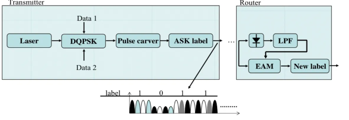
1-3 New scheme to generate DQPSK payload/ASK label signal

Laser DQPSK Pulse carver ASK label … Data 1

Data 2

LPF

EAM New label

label 1 0 1 1

Transmitter Router

Fig 1-2 Structure of RZ-DQPSK/ASK label signal transmitter and router

The RZ-DQPSK/ASK label signal transmitter and label router setup is shown Fig 1-2 However, to implement such an ASK/RZ-DQPSK orthogonal modulation format, three cascaded optical modulators are required for phase encoding, pulse carving and label impressing, an arrangement that is extremely costly and difficult to manage due to the size and the electronic components required in each modulator. In addition, the heritage loss is usually so high that two EDFAs will be needed in the transmitting end. This thesis proposes a simple and elegant method to generate ASK/RZ-DQPSK signal which used the two dual-drive Mach-Zehnder modulator. The first Mach-Zehnder modulator generates NRZ-DQPSK. The second Mach-Zehnder modulator is used to impress the label data and perform pulse carving. First, the sin wave mix the low bit rate label data used mixer into Mach-Zehnder modulator before.

Chapter 2

DQPSK payload/ASK label signal

2-1 Mach-Zehnder modulator

At bit rates of 10 Gb/s or higher, the frequency chirp imposed by direct modulation becomes large enough that direct modulation of semiconductor lasers is rarely used. For such high-speed transmitters, the laser is biased at a constant current to provide the CW output, and an optical modulator placed next to the laser converts the CW light into a data-coded pulse train with the right modulation format. The most commonly used Mach-Zehnder external modulators are based on LiNbO3 (lithium niobate) technology, therefore this section will deal only with these types of devices.

The linear electro-optic effect that is used to produce the phase changes in the branches of the Mach-Zehnder modulator is known as the “Pockels-effect”. For LiNbO3, the application of an electric field results in a change in the refractive index and therefore varies the phase of the propagating light. The strength of this electro-optic effect is dependent on the direction of the applied electric field and the orientation of the LiNbO3 crystal. Hence, the electrode placement and configuration is a critical design issue.

Intensity trimmer Intensity trimmer

Fig 2-1 The Mach-Zehnder modulator having two intensity trimmers

Fig 2-1 shows a Mach-Zehnder modulator having two intensity trimmers in the arms. By using the trimmers, we can compensate the amplitude imbalance due to fabrication

errors, where the intensity trimmers can be also constructed byMZ structures.

The most general case is a dual-drive modulator with two possibly independent drive signals. Where the dual-drive modulator formula is:

1 2 1 2 1 2 2 0 0 1 1 cos 2 2 2 j L j L j L E E e e E L e φ φ φ φ

φ

φ

Δ +Δ ⋅ Δ Δ Δ − Δ ⎧ ⎫ ⎛ ⎞ = _⎨ + _⎬= ⋅ _⎜ ⋅ _⎟⋅ ⎩ ⎭ ⎝ ⎠ (1) 2 _{2 1 2} 0 cos 2 power= E ⎛_⎜Δ − Δ

φ

φ

⋅L⎞_⎟ ⎝ ⎠ (2) 1 2 2 phase modulation: Δ Δ j L

e

φ+ φ _⋅ − (3) 1 2

amplitude modulation: cos

2 L φ φ Δ − Δ ⎛ ⎞ − _⎜ ⋅ _⎟ ⎝ ⎠ (4)

2-2 Differential quadrature phase shift keying (DQPSK)

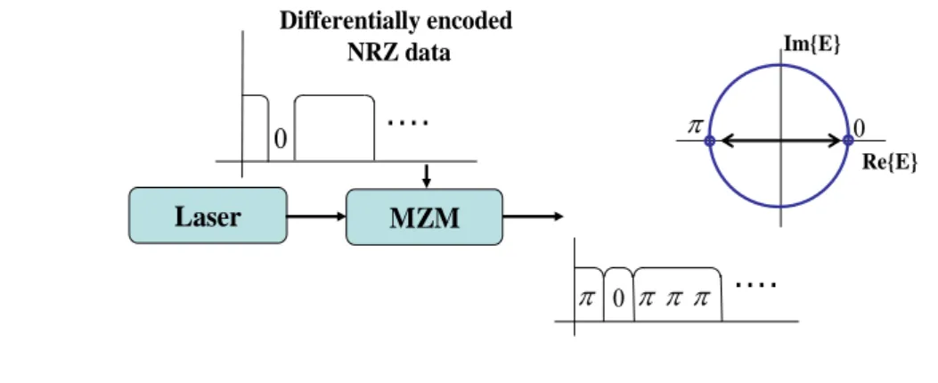
In the case of PSK (phase shift keying) format, the optical bit stream by modulating the phase while the amplitude and the frequency of the optical carrier are kept constant. For binary PSK, the phase takes two values, commonly chosen to be 0 andπ. The PSK formats carry the information in the optical phase itself. Due to the lack of an absolute phase reference in direct-detection receivers, the phase of the preceding bit is used as a relative phase reference for demodulation. This results in differential phase shift keying (DPSK) formats, which carry the information in optical phase changes between bits. The commonly used DPSK transmitter setups are shown in Fig 2-2. The transmitters consist of a continuously oscillating laser followed by one external modulator, typically based on LiNbO3 technology. Phase modulation can either be performed by a

Laser MZM Differentially encoded NRZ data

….

0

….

π 0 π π π Im{E} Re{E} π 0

Fig 2-2 the DPSK transmitter and DPSK modulation

There have been a number of applications that have been propose and demonstrated for PSK. One of these is to increase spectral efficiency through the use of multilevel signaling is DQPSK. The basic principle of optical DQPSK (differential quadrature phase shift keying) modulation is to represent each couple of two bits (so called “dibit”) of the information sequence to be transmitted by optical phase differences between consecutive symbols taking values into ,0, ,

2 2

π _{π π}

⎧₋ ⎫

⎨ ⎬

⎩ ⎭.Each transmitted symbol therefore corresponds to two bits of information, meaning that the symbol rate (in baud) is equal to half of the bit rate (B, in bit/s).

The Fig 2-3 illustrates the partitioning of a typical pulse stream for DQPSK modulation. Fig 2-3(a) shows the original data stream d t_k

( )

=d d d₀, , ,..._{1 2} consisting of bipolar pulses; that is, the values of d t binary one and zero, respectively. The pulse stream is _k

( )

divided into an in-phase stream,d t , and a quadrature stream,_I

( )

d t , illustrated in Fig _Q

( )

2-3(b), as follows:

( )

( )

0 2 4 1 3 5 , , ,... ( ) , , ,... ( ) I Q d t d d d even bit d t d d d odd bit = =

Note that d t and _I

( )

d t each have half the bit rate of_Q

( )

d t . _k

( )

Fig 2-3 (a) QPSK modulation (b) in-phase stream and quadrature stream

0 d d1 d2 d3 d4 d5 d6 d7 1 0 T 2T 3T 4T 5T 6T 7T 8T t 0 d d2 d4 d6 1 0 2T 4T 6T 8T t

( )

k d t ( ) I d t 1 d d3 d5 d7 1 0 2T 4T 6T 8T t

( )

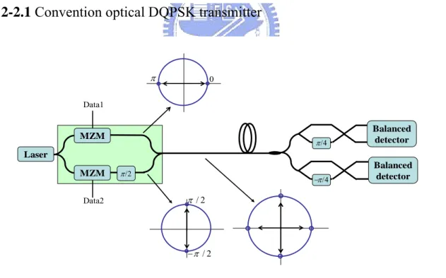
Q d t (a) (b)

2-2.1 Convention optical DQPSK transmitter

π 0 Laser MZM MZM π/2 Data1 Data2 π / 2 / 2 π −

Fig 2-4 The structure of an optical DQPSK system

/4 π /4 π − Balanced detector Balanced detector

The transmitter consists of two parallel DPSK modulators that are integrated together in order to achieve phase stability (a serial arrangement is also possible, and has been used in experimental demonstrations).

The electric field of DPSK signal at the modulator output is

( )

( )

1 ( ) exp exp 2 2 2 j j e t = ⎧_{⎨ ⎢}⎡ πφ t _⎥⎤− _⎢⎡− πφ t ⎤_⎥⎫_⎬ ⎣ ⎦ ⎣ ⎦ ⎩ ⎭ (6) Now consider, t he electric field of QPSK signal at the modulator output is

( )

( )

( )

( )

( )

( )

( )

( )

1 2 1 1 2 2 1 2 ( ) 1 exp exp 2 2 2 1 exp exp 2 2 2 sin cos 2 2 E t e t je t j j t t j j j t t t t π_φ π_φ π_φ π_φ π_φ π_φ = + ⎧ ⎡ ⎤ ⎡ ⎤⎫ = _{⎨ ⎢ ⎥}− _⎢− _⎥⎬ ⎣ ⎦ ⎣ ⎦ ⎩ ⎭ ⎧ ⎡ ⎤ ⎡ ⎤⎫ + _{⎨ ⎢ ⎥}− _⎢− _⎥⎬ ⎣ ⎦ ⎣ ⎦ ⎩ ⎭ ⎡ ⎤ ⎡ ⎤ = _{⎢ ⎥}+ _{⎢ ⎥} ⎣ ⎦ ⎣ ⎦ (7)

( )

t

φ is the normalized binary drive signal

( )

( )

(

)

n n k k t b p t kT φ +∞ =−∞ =

∑

− (8) Where b_{n k( )} = ± is the transmitted random data stream, 1 p t is the pulse shape of

( )

the drive signal, n=1 and 2, and T is the bit interval of the data. The receiver essentially consist of two DPSK receivers, although the phase difference in the arms of the delay interferometers is now set to +π/ 4 and−π/ 4. Whose differential delay is equal to the bit period. The benefit of DQPSK is that, for the same data rate, the symbol rate is reduced by a factor of two.

2-2.2 Variety of dual-drive DQPSK signals

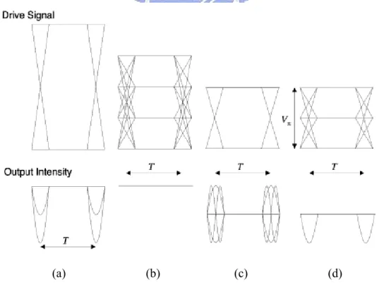
A DQPSK signal can also be generated using a conventional dual-drive Mach-Zehnder modulator. The dual-drive Mach-Zehnder modulator consists of two

phase modulators that can be operated independently. The Fig 2-5 shows the three kinds of method to generate DQPSK signals and the conventional method to generate DQPSK signals, which are the eye diagram of the drive signal and output intensity of the DPQSK transmitter. The fig2-5(a) is used with two two-level drive signals having a peak to peak drive voltage of 2V_π. The fig 2-5 (b), (c) and (d) separately represent to drives the dual-drive Mach-Zehnder modulator with a four-level drive signal, two-level drive signal and three-level drive signal. The peak to peak drive voltage is reducing from 1.5V_π for four-level signal to V_π for two- and three- level drive signals. The output intensity of conventional transmitter has optical intensity ripples between consecutive symbols. With two or three levels of drive signal, the output intensity of the dual-drive Mach-Zehnder modulator also has ripples between consecutive symbols.

(a) (b) (c) (d)

Fig 2-5 Eye diagram of the drive signal and output intensity, where (a) the conventional transmitter and dual-drive transmitter (b) four-, (c) two-, and (d) three-level drive signals

2-2.3 Two level drive DQPSK transmitter

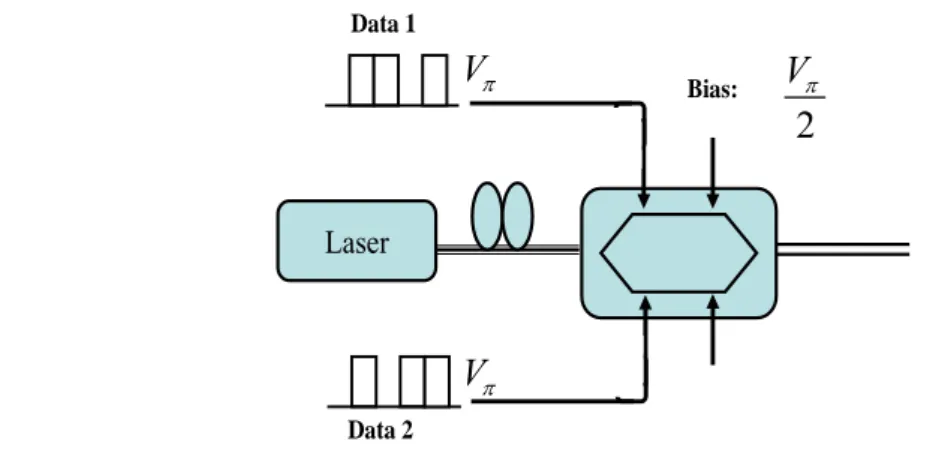
We focused how to generate DQPSK signals which used two-level drive signals at this thesis. The Fig 2-6 shows the input data streams and bias point of the dual-drive Mach-Zehnder modulator to generate DQPSK signals. First, a continuous wave is externally modulated by a dual-drive Mach-Zehnder modulator. Biased at the quadrature, the two arms of the MZM are fed by two independent data streams, V1 and V2, and each

with peak to peak amplitude (Vpp) equals to the switching voltage, Vπ.

Data 1

2

V

_π Bias: Data 2

V

_π

V

_π Laser

Fig 2-6 Two-level drive signals used one dual drive Mach-Zehnder modulator

The output electrical field can be written as:

1 2 2 1 2 cos 2 b V V V j V b out in V V V E E e V π π π π ⎛ + + ⎞ ⎜ ⎟ ⎝ ⎠ ⎛ − + ⎞ = _{⎜ ⎟} ⎝ ⎠ (9) Where V_b =V_π / 2 is the biased voltage.

Now we consider four cases ( the input data1 is zero and data2 is zero, the input data1 is zero and data2 is one, the input data1 is one and data2 is zero and the input data1 is one and data2 is one ) in two independent data streams.

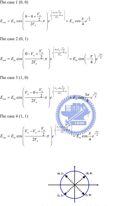
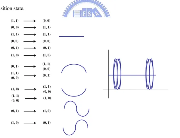
The case 1 (0, 0) 0 0 2 2 4 0 0 2 cos cos 2 4 V j V j out in in V E E e E e V π π π π _π π π π ⎛ _{+ +} ⎞ ⎜ ⎟ ⎜ ⎟ ⎜ ⎟ ⎜ ⎟ ⎝ ⎠ ⎛ _{− +} ⎞ ⎜ ⎟ = _{⎜ ⎟} = ⎜ ⎟ ⎝ ⎠ (10) The case 2 (0, 1) 0 2 3 2 4 0 2 cos cos 2 4 V V j V _j out in in V V E E e E e V π π π π π _π π π π π ⎛ _{+ +} ⎞ ⎜ ⎟ ⎜ ⎟ ⎜ ⎟ ⎜ ⎟ ⎝ ⎠ ⎛ _{− +} ⎞ ⎜ ⎟ _{⎛ ⎞} = _{⎜ ⎟} = _⎜− _⎟ ⎝ ⎠ ⎜ ⎟ ⎝ ⎠ (11) The case 3 (1, 0) 0 2 3 2 4 0 ₃ 2 cos cos 2 4 V V j V _j out in in V V E E e E e V π π π π π _π π π π π ⎛ _{+ +} ⎞ ⎜ ⎟ ⎜ ⎟ ⎜ ⎟ ⎜ ⎟ ⎝ ⎠ ⎛ _{− +} ⎞ ⎜ ⎟ = _{⎜ ⎟} = ⎜ ⎟ ⎝ ⎠ (12) The case 4 (1, 1) 2 5 2 4 2 cos cos 2 4 V V V j V _j out in in V V V E E e E e V π π π π π π _π π π π π π ⎛ _{+ +} ⎞ ⎜ ⎟ ⎜ ⎟ ⎜ ⎟ ⎜ ⎟ ⎝ ⎠ ⎛ _{− +} ⎞ ⎜ ⎟ = _{⎜ ⎟} = ⎜ ⎟ ⎝ ⎠ (13) (0, 0) (1, 0) (0, 1) (1, 1)

Fig 2-7 the symbol constellation of DQPSK signal

the second coordinates, the (0, 1) case is at the third coordinates and the (1, 1) case is at the forth coordinates. The Fig 2-7 illustrates the symbol constellation of DQPSK signal, which has four phases depending on the input signal V1 and V2.

2-2.4 Transition of two level drive DQPSK

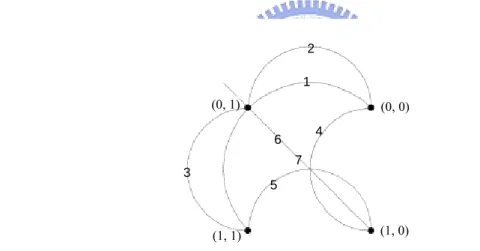
The two-level scheme has overshoot ripples doubling the output intensity. Those variations of electric field are equivalent to frequency chirp. The output intensity of two-level scheme has five kind of power fluctuates that show in Fig 2-5(c). This thesis provides two kind of methods to discuss how to happen overshoot ripples when symbol change to another symbol. First, the Fig 2-8 shows the symbol constellation with electric field locus of a dual-drive transmitter.

1 2 3 4 5 6 7 (0, 0) (0, 1) (1, 0) (1, 1)

Fig 2-8 the symbol constellation with electric field locus of a dual-drive transmitter

When symbol (0, 0) change to symbol (1, 1), the electric field locus follow route 1 to arrive symbol (1, 1) simultaneously, vice versa. The output intensity of DQPSK signal is constant power at transition state. When the symbol (0, 0) change to (0, 1), the electric field locus follow route 2 to arrive symbol (0, 1) simultaneously, vice versa. When the symbol (1, 1) change to (0, 1), the electric field locus follow route 3 to arrive symbol (0, 1) simultaneously, vice versa. The output intensities of route 2 and route 3 will increase

to maximum value at transition state. When the symbol (0, 0) change to (1, 0), the electric field locus follow route 4 to arrive symbol (1, 0) simultaneously, vice versa. When the symbol (1, 1) change to (1, 0), the electric field locus follow route 5 to arrive symbol (1, 0) simultaneously, vice versa. The output intensities of route 4 and route 5 will reduce to minimum value at transition state. When the symbol (0, 1) change to (1, 0), the electric field locus follow route 6 to arrive symbol (1, 0) simultaneously. The output intensities will reduce to minimum value then increase to maximum value at transition state. When the symbol (1, 0) change to (0, 1), the electric field locus follow route 6 to arrive symbol (0, 1) simultaneously. The output intensities will increase to maximum value then reduce to minimum value at transition state. When symbol does not change its state, the output intensity is constant power at transition state.

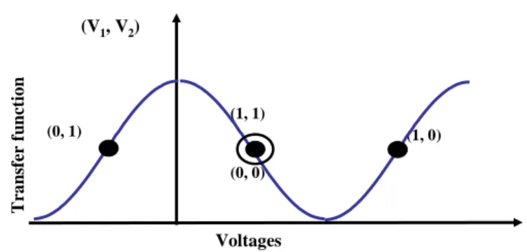
We also can use symbol position of Mach-Zehnder modulator transfer curve that shows in Fig 2-9. Since the symbol transition passes through the minimum and the maximum of the transfer curve, the power fluctuates around the symbol edge owing to the rise-fall time of the drive signal.

(0, 0) (1, 1) (0, 1) _{(1, 0)} (V₁, V₂) Voltages Tr an sf er f u nc tion

Fig 2-9 The symbol position of Mach-Zehnder modulator transfer function

The symbol (0, 0) and symbol (1, 1) position were at V_π/ 2 of Mach-Zehnder modulator transfer curve, so that the output intensities are constant power at transition

state of symbol (0, 0) to symbol (1, 1) or symbol (1, 1) to symbol (0, 0). The symbol (0, 1) position is at −V_π / 2 of Mach-Zehnder modulator transfer curve, so that the output intensities will increase to maximum value at transition state of symbol (0, 0), symbol (1, 1) to symbol (0, 1) or symbol (0, 1) to symbol (0, 0), symbol (1, 1). The symbol (1, 0) position is at 3 / 2V_π of Mach-Zehnder modulator transfer curve, so that the output intensities will reduce to minimum value at transition state of symbol (0, 0), symbol (1, 1) to symbol (1, 0) or symbol (1, 0) to symbol (0, 0), symbol (1, 1). The symbol (0, 1) to symbol (1, 0) will follow transfer curve which increase to maximum value then reduce to minimum value at transition state. Adversely, the symbol (1, 0) to symbol (0, 1) also will follow transfer curve which reduce to minimum value then increase to maximum value at transition state. (1, 1) (0, 0) (0, 0) (1, 1) (1, 1) (1, 1) (0, 0) (0, 0) (0, 1) (0, 1) (1, 0) (1, 0) (0, 1) (1, 1) (0, 0) (1, 1) (0, 1) (0, 0) (1, 0) (1, 1) (0, 0) (1, 1) (1, 0) (0, 0) (0, 1) (1, 0) (1, 0) (0, 1)

Fig 2-10 the five kind power fluctuates of symbol transition

that shows in Fig 2-10. The overshoot ripples between symbols will influence NRZ-DQPSK signal quality so that the dual-drive Mach-Zehnder modulator pulse carver will change NRZ-DQPSK to RZ-DQPSK signal.

2-2.5 Eye spreading of two level drive DQPSK

The ripple of the drive signal transfer to the optical signal. With the conventional transmitter, no amplitude ripple of the drive signal transfers to the phase ripple. Even when the drive signal has a large ripple, the intensity ripple of the transmitted signal is compressed by the nonlinear transfer function of Mach-Zehnder modulator. For the NRZ-DQPSK signal, the ripples from the drive signal may be increase by the Mach-Zehnder modulator. This section will discuss and calculate optical eye spreading of NRZ-DQPS. The eye spreading is defined asΔ =_e (δ δ₁+ ₂) /d, where δ₁ and δ₂ are the spreading in the upper and lower level, and d is the high of the eye diagram, the Fig 2-11 shows eye spreading of the two-level eye spreading.

Fig 2-11 eye spreading of the two-level eye spreading

Assume δ₁=δ₂→ = Δδ _ed/ 2

(14)

Consider bias point is V_b =d/ 2 into 2_{cos (}2 ₎

2 b e V P E V_π δ+ _π = (15) 2_{cos (}2 / 2 / 2 ₎ 2 e e d d P E d π Δ + → = 2_{cos (}2 1 ₎ 4 e e P E Δ + π → =

2 1 1 cos( ) 2 ( ) 2 e e P E π Δ + +

→ = cos( 1 ) cos( ) cos( ) sin( )sin( )

2 2 2 2 2 e π eπ π eπ π Δ + Δ Δ → = − 1 cos( ) sin( ) 2 2 e π eπ Δ + Δ → = − (16) Assume sin( ) 2 2 eπ eπ Δ Δ − = − 2₍1 2 ₎ 2₍1 ₎ 2 2 4 e e e e P E π E π Δ − _Δ → = = − (17) Because 1/2 is influence of bias point, we don’t consider this item.

2 4 e e P_δ E Δ π → = −

Now NRZ eye spreading is defined as:

2 2 2( ) 4 2 e e onrz e e E E π π Δ − Δ = = −Δ

(18)

After calculating, the NRZ-DQPSK eye spreading Δ will simplify to _nrz Δ _eπ

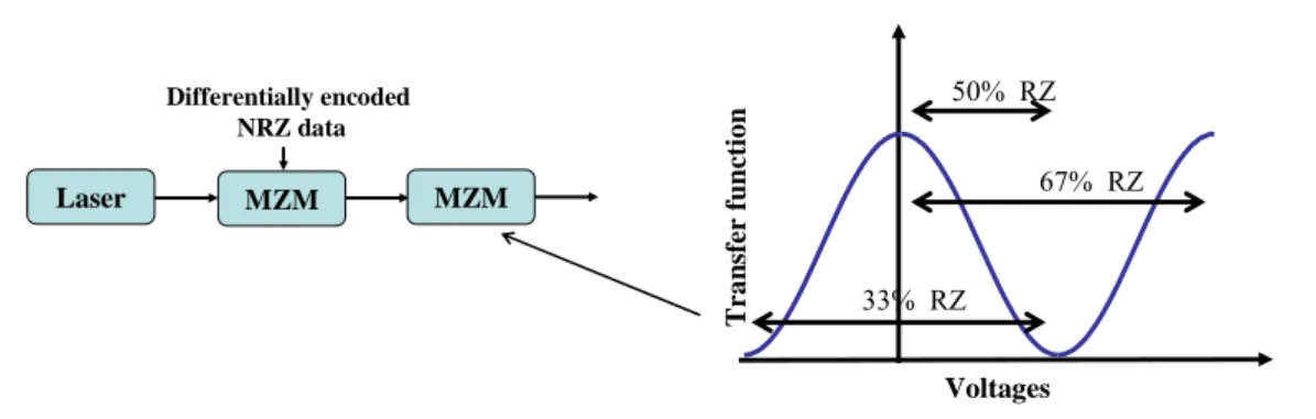
2-3 Pulse carver for RZ-DQPSK

Since DQPSK carries information in the phase of the optical signal, optical phase distortions (such as chirp) will have a severe impact on DQPSK receiver performance. At the transmitter, phase distortions may be caused by imperfect pulse carvers.

In order to operate chirp-free, a dual-drive MZM pulse carver has to have infinite DC

extinction, and has to work in perfect push-pull operation, i.e., the sinusoidal drive amplitudes have to be of the same amplitude and of opposite phase. The Fig. 2-12 shows

MZM-based pulse carver. The resulting RZ duty cycles are 33%, 50%, and 67%. Voltages T ran sf er fu nc ti on 50% RZ 67% RZ 33% RZ Laser MZM Differentially encoded NRZ data MZM

Fig 2-12 Three commonly used ways of pulse carving by applying MZM-based pulse carver

Three important facts are evident from the optical intensity and phase waveforms shown in Fig 2-13: First, when sinusoidally carving at the data rate (50% RZ), the residual optical phase variations are identical for each bit, while they are different for adjacent bits when carving at half the data rate (33% and 67% RZ). Since it is the difference between the optical phases of two adjacent bits that is used to decode DPSK signals at the receiver, higher degradations due to pulse carver chirp are found for 33% and 67% duty cycle RZ-DQPSK than for 50% RZ-DQPSK. Second, we see from the opposite phase curvatures (50% and 67%) or slope (33%) that chirp due to finite DC extinction ratios of the MZM can partially be compensated by imbalancing the drive amplitudes. Third, we notice that for 33% RZ a drive-signal amplitude imbalance leads to linear phase transitions (i.e., to optical frequency shifts) at pulse center, while a drive-signal phase error produces a phase offset at pulse center. Since pure bit-alternating frequency offsets do not disturb the phase difference between adjacent bits at pulse center (where the intensity is highest, and thus the contribution to the demodulated signal is largest), a higher tolerance is found for drive amplitude imbalance than for drive phase errors in the case of 33% RZ. For 67% RZ, the situation is opposite, and we find a higher tolerance to

drive phase errors than to drive amplitude imbalance.

Fig 2-13 the optical intensity and phase waveforms (50% RZ, 33% RZ and 67%RZ)

2-4 DQPSK demodulation

A typical balanced DQPSK receiver is shown in Fig. 2-14. The receiver essentially consist of two DPSK receivers, although the phase difference in the arms of the Mach-Zehnder delay-interferometer (DI) is now set to +π/ 4 and−π/ 4. The optical signal is first passed through a Mach-Zehnder delay-interferometer (DI), whose differential delay is equal to the bit period. This optical preprocessing is necessary in direct-detection receivers to accomplish demodulation, since photodetection is inherently insensitive to the optical phase; a detector only converts the optical signal power into an electrical signal. In a direct-detection DQPSK receiver, the DI lets two adjacent bits interfere with each other its output ports. This interference leads to the presence (absence) of power at a DI output port if two adjacent bits interfere constructively (destructively) with each other.

/4 π /4 π − Balanced detector Balanced detector RZ-DQPSK signal

Fig 2-14 typical balanced DQPSK receiver

Thus, the preceding bit in a DQPSK-encoded bit stream acts as the phase reference for demodulating the current bit. (Note that in the case of coherent detection, this phase reference can be provided by a local laser within the receiver, which beats with the received signal to produce constructive and destructive interference.)

Ideally, one of the DI output ports is adjusted for destructive interference in the absence of phase modulation (“destructive port”), while the other output port then automatically exhibits constructive interference due to energy conservation (“constructive port”). For the same reason, the two DI output ports will carry identical, but logically inverted data streams under DQPSK modulation.

Now we consider DI how to determine 0 and 1, that the RZ-DQPSK signal through Mach-Zehnder delay-interferometer. The optical signal is first passed through a Mach-Zehnder delay-interferometer whose differential delay is equal to the bit period and does not delay bit will rotate +π/ 4 and−π/ 4. The intensity of two bit through Mach-Zehnder delay-interferometer compose vector will decide the zero and one The Fig 2-15 shows the constellation of zero and one determined method. Assume into Mach-Zehnder delay-interferometer signal sequence is the symbol (0, 1) and the symbol

(0, 0). That rotated +π/ 4 and−π/ 4 represents the transmitter input two kind of data, data1 and data2.

(0, 0) (0, 1)

(0, 0) (0, 1)

(a) (b)

The Fig 2-15 the constellation of zero and one determined method (a) rotated ,the composed vector is zero, (b) rotated , the composed vector is one

/ 4 π − /4 π +

Every symbol change to another symbol has sixteen case of symbol changing totally. The constellation do not consider phase, the large compose vectors represent one and the large compose vectors represent zero.

2-5 Structure of DQPSK/ASK Label

Future Internet routers will need optical label switching to route and forward a massive number of packets per second independently of IP packet length and payload bit rate. Orthogonal amplitude shift keying /differential quadrature phase shift keying (ASK/DQPSK) optical label has been proposed as a competing scheme to sub-carrier multiplexed optical label due to its compact spectrum, simple label swapping and remarkable scalability to high bit rates.

At the ingress edge router, the incoming IP packets are assigned an amplitude shift keying (ASK) label, orthogonally modulated to the RZ-DQPSK payload. The packet switched network architecture requires the optical label to be swapped during the routing process to establish an appropriate optical path through the transmission fiber

network, as shown in the Fig. 2-16. node A node B edge router core router fiber _fiber ASK label A

RZ-DQPSK payload ASK label B RZ-DQPSK payload Fig 2-16 system architecture for DQPSK/ASK label signal

The high speed packet data is in DQPSK format, while the low speed label is written with a low extinction ratio amplitude shift keying format. At network nodes, the label read by detecting and low pass filter some fraction of the signal. The label on the routed signal can then be erased and rewritten using an intensity modulator. At the packet destination, the data is read using a DQPSK receiver. The RZ-DQPSK/ASK label signal transmitter and label router setup is shown Fig 2-17.

Laser DQPSK Pulse carver ASK label …

Data 1

Data 2

LPF

EAM New label

label 1 0 1 1

Transmitter Router

2-5.1 Simple RZ-DQPSK/ASK Label transmitter

However, to implement such an ASK/RZ-DQPSK orthogonal modulation format, three cascaded optical modulators are required for phase encoding, pulse carving and label impressing, an arrangement that is extremely costly and difficult to manage due to the size and the electronic components required in each modulator. In addition, the heritage loss is usually so high that two EDFAs will be needed in the transmitting end. This thesis proposes a simple and elegant method to generate ASK/RZ-DQPSK signal which used the two dual-drive Mach-Zehnder modulator. The first Mach-Zehnder modulator generates NRZ-DQPSK. The second Mach-Zehnder modulator is used to impress the label data and perform pulse carving. First, the sin wave mix the low bit rate label data used mixer into Mach-Zehnder modulator before. Thus the pulse will include ASK label signal is shown the Fig 2-18.

Laser DQPSK Pulse carver … Data 1

Data 2

label 1 0 1 1 Transmitter

Fig 2-18 The simple RZ-DQPSK/ASK label signal transmitter ASK label Sinwave (bate/2HZ)

Chapter 3

Experiment setup and result (DQPSK)

3-1 Dual-Drive DQPSK experiment setup

DQPSK Payload 20 Gb/s Clock DQPSK Transmitter 80-km SSMF DCF Payload Decision DQPSK Receiver EDFA OBPF +π/4 -π/4 Payload Decision delay

The Fig 3-1 Dual-Drive DQPSK signal experiment setup

The experimental setup is shown in the Fig 3-1, which mainly contains three part: payload transmitter, transmission fiber, and payload receiver. The RZ-DQPSK transmitter consists of continuously oscillating laser at 1546.96nm, two external dual-drive Mach-Zehnder modulators. The first modulator generates a 20Gbit/s NRZ-DQPSK signal. Biased atV_π / 2, two independent electrical data streams, which is driven by 10Gbit/s (PRBS ₂15_{− ) NRZ data stream individually. The second 1}

modulator generates a 10GHz RZ pulse train with 33% (The modulator is biased at the peak of its transmission curve and differentially driven at twice the switching voltage with an AC-coupled half-bitrate 5GHz sine wave), 50% (The modulator is biased at the linear range of its transmission curve and differentially driven at twice the switching

voltage with an AC-coupled 10GHz sine wave) and 67% (The modulator is biased at the null point of its transmission curve and differentially driven at twice the switching voltage with an AC-coupled half-bitrate 5GHz sine wave)duty cycle. A tunable optical delay line is inserted in between the two modulators to synchronize the pulse train and the 20Gbit/s data. There is place boot amplifier before the transmission fiber and control appropriate power.

The transmission span consists of 82km standard singlemode fiber with matching length of 14.564km dispersion compensating fiber (DCF) in a post compensation scheme. The fiber loss of the singlemode fiber and the dispersion compensating fiber is 16.54dB and 6.18dB, respectively.

The RZ-DQPSK receiver consists of pre-amplifier, the optical band pass filter, two integrated Mach-Zehnder delay interferometer (the phase difference in the arms of the Mach-Zehnder delay-interferometer (DI) is now set to +π/ 4 and−π/ 4), the photo detector, and the BER tester. The bandwidth of optical band pass filter is 40GHz. The payload is then input to an integrated Mach-Zehnder delay interferometer to demodulate the RZ-DQPSK signal. The length difference between the two arms of the MZDI is corresponding to 100ps delay. The signal at the output of MZDI is detected by photo detector and input to a 10Gbit/s BER test.

(a) eye diagram of MZM electrical driver

0.4V

(b) eye diagram of NRZ-DQPSK signal

0.4V 5V 0.789mW 1.575mW 5V 0.789mW 1.575mW

The Fig 3-2 (a) eye diagram of MZM electrical driver (b) eye diagram of NRZ-DQPSK signal

The Fig 3-2(b) shows the eye diagram of NRZ-DQPSK signal. We measure optical eye spreading to compare with the eye spreading using electrical eye spreading calculated value. Using 1 2 ( ) / (0.4 0.4) / 5 16% e δ δ d Δ = + = + = 0.16*3.14 50.02% onrz eπ Δ = −Δ = =

The measure value is corroding to calculated value. 0.789 /1.575 0.5 50%

onrz

Δ = = =

3-2 Spectrum of DQPSK demodulation

Fig 3-3 the spectrum of DQPSK signal demodulation

delay-interferometer demodulation. The phase is set to +π/ 4 of Mach-Zehnder delay-interferometer whose constructive port is 45° and destructive port is -135°. Thus the phase is set to −π/ 4 of Mach-Zehnder delay-interferometer whose constructive port is 45° and destructive port is 135°. The two ports (constructive and destructive) of Mach-Zehnder delay-interferometer are differing 180°, which like the Fig 2-14 shown.

3-3 Sensitivity of Dual-drive DQPSK

3-3.1 DD NRZ DQPSK

The Fig 3-4 shows eye diagram for NRZ-DQPSK demodulation. The Fig 3-4(a) is the phase set to −π/ 4 of Mach-Zehnder delay-interferometer whose destructive port is135°. The Fig3-4(b) is the phase set to +π/ 4 of Mach-Zehnder delay-interferometer whose destructive port is -135°.

The Fig 3-5 shows the BER curves for NRZ-DQPSK in the back to back case. The sensitivity of 135° case is -24dBm, and the sensitivity of -135° case is -24.8dBm. There are differing about 0.8dB penalty. After averaging, the sensitivity of NRZ-DQPSK in the back to back case is -24.3dBm.

(a) Eye diagram ( 135° ) for NRZ-DPQSK demodulation

(b) Eye diagram ( -135° ) for NRZ-DPQSK demodulation

-31 -30 -29 -28 -27 -26 -25 -24 -23 10-11 10-10 10-9 10-8 10-7 10-6 10-5 10-4 10-3 Received Power (dBm) BE R 135 -135 AVERAGE Fig 3-5 BER of DD NRZ-DQPSK

3-3.2 DD 33%RZ DQPSK

The Fig 3-6 shows eye diagram for 33% RZ-DQPSK demodulation. The Fig 3-6(a) is the phase set to −π/ 4 of Mach-Zehnder delay-interferometer whose destructive port is 135° and the Fig 3-6(b) constructive port is -45°. The Fig 3-6(c) is the phase set to

/ 4 π

+ of Mach-Zehnder delay-interferometer whose destructive port is -135° and the Fig 3-6(d) constructive port is 45°.

The Fig 3-7 shows the BER curves for 33% RZ-DQPSK in the back to back case. The sensitivity of 135° case is -29.1dBm, the sensitivity of -45° case is -29.2dBm, the sensitivity of -135° case is -28.9dBm, and the sensitivity of 45° case is -29.6dBm. The worst case (-135) and the best case (45) are differing maximum value which plenty is

about 0.9dB. After averaging, the sensitivity of 33% RZ-DQPSK in the back to back case is -29.11dBm.

(a) Eye diagram ( 135° ) for 33% RZ-DPQSK demodulation

(b) Eye diagram ( -45° ) for 33% RZ-DPQSK demodulation

(c) Eye diagram ( -135° ) for 33% RZ-DPQSK demodulation

(d) Eye diagram ( 45° ) for 33% RZ-DPQSK demodulation The Fig 3-6 Eye diagram for DD 33% RZ-DQPSK demodulation

-35 -34 -33 -32 -31 -30 -29 -28 10-11 10-10 10-9 10-8 10-7 10-6 10-5 10-4 Received Power (dBm) BE R 10-11 10-10 10-9 10-8 10-7 10-6 10-5 10-4 10-11 10-10 10-9 10-8 10-7 10-6 10-5 10-4 135 -45 -135 45 AVERAGE Fig 3-7 BER of DD 33% RZ-DQPSK

3-3.3 DD 50%RZ DQPSK

The Fig 3-8 shows eye diagram for 50% RZ-DQPSK demodulation. The Fig 3-8(a) is the phase set to −π/ 4 of Mach-Zehnder delay-interferometer whose destructive port is 135° and the Fig 3-8(b) constructive port is -45°. The Fig 3-8(c) is the phase set to

/ 4 π

+ of Mach-Zehnder delay-interferometer whose destructive port is -135° and the Fig 3-8(d) constructive port is 45°.

The Fig 3-9 shows the BER curves for 50% RZ-DQPSK in the back to back case. The sensitivity of 135° case is -28.1dBm, the sensitivity of -45° case is -28.1dBm, the sensitivity of -135° case is -28.2dBm, and the sensitivity of 45° case is -28dBm. The worst case (-135) and the best case (45) are differing maximum value which plenty is about 0.2dB. After averaging, the sensitivity of 50% RZ-DQPSK in the back to back case is -28.1dBm.

(a) Eye diagram ( 135° ) for 50% RZ-DPQSK demodulation

(b) Eye diagram ( -45° ) for 50% RZ-DPQSK demodulation

(c) Eye diagram ( -135° ) for 50% RZ-DPQSK demodulation

(d) Eye diagram ( 45° ) for 50% RZ-DPQSK demodulation

-34 -33 -32 -31 -30 -29 -28 -27 -26 10-12 10-11 10-10 10-9 10-8 10-7 10-6 10-5 10-4 Received Power (dBm) BE R 135 -45 -135 45 AVERAGE Fig 3-9 BER of DD 50% RZ-DQPSK

3-3.4 DD 67%RZ DQPSK

The Fig 3-10 shows eye diagram for 67% RZ-DQPSK demodulation. The Fig 3-10(a) is the phase set to −π/ 4 of Mach-Zehnder delay-interferometer whose destructive port is 135° and the Fig 3-10(b) constructive port is -45°. The Fig 3-10(c) is the phase set to +π/ 4 of Mach-Zehnder delay-interferometer whose destructive port is -135° and the Fig 3-10(d) constructive port is 45°.

The Fig 3-11 shows the BER curves for 67% RZ-DQPSK in the back to back case. The sensitivity of 135° case is -27.3dBm, the sensitivity of -45° case is -27.1dBm, the sensitivity of -135° case is -26.7dBm, and the sensitivity of 45° case is -27.3dBm. The worst case (-135) and the best case (45and 135) are differing maximum value which

plenty is about 0.6dB. After averaging, the sensitivity of 67% RZ-DQPSK in the back to back case is -27dBm.

(a) Eye diagram ( 135° ) for 67% RZ-DPQSK demodulation

(b) Eye diagram ( -45° ) for 67% RZ-DPQSK demodulation

(c) Eye diagram ( -135° ) for 67% RZ-DPQSK demodulation

(d) Eye diagram ( 45° ) for 67% RZ-DPQSK demodulation

The Fig 3-10 Eye diagram for DD 67% RZ-DQPSK demodulation

-33 -32 -31 -30 -29 -28 -27 -26 -25 10-12 10-11 10-10 10-9 10-8 10-7 10-6 10-5 10-4 Received Power (dBm) BE R 135 -45 -135 45 AVERAGE Fig 3-11 BER of DD 67% RZ-DQPSK

3-3.5 Transmission penalty of dual-drive DQPSK

The eye diagrams through 80km transmission are shows the Fig3-12. The Fig 3-13 shows the BER curves in the back to back case and after transmission over 80km. For a NRZ-DQPSK signal, the back-to-back sensitivity is -25.5dBm and the transmission sensitivity is -25.5dBm. For a 33%RZ-DQPSK signal, the back-to-back sensitivity is -29.3dBm and the transmission sensitivity is -28.6dBm. The penalty is 0.6dB. For a 50%RZ-DQPSK signal, the back-to-back sensitivity is -28.8dBm and he transmission sensitivity is -28.6dBm. The penalty is 0.2dB. For a 67%RZ-DQPSK signal, the back-to-back sensitivity is -26.4dBm and he transmission sensitivity is -26.4dBm. The penalty of NRZ and 67% cases are 0dB.

(a) Eye diagram of NRZ-DQPSK after 80km transmission (b) Eye diagram of 33%RZ-DQPSK after 80km transmission (c) Eye diagram of 50%RZ-DQPSK after 80km transmission (d) Eye diagram of 67%RZ-DQPSK after 80km transmission

3-4 Timing misalignment of dual-drive DQPSK

The timing misalignment causes phase discontinuity at the pulse shift and make the eye diagram of the received signal closed. The Fig 3-14 shows power penalty for 33%, 50% and 67% RZ-DQPSK signal measured as a function of timing delay form the optimal condition that offers continuous- phase modulation. For 33%RZ-DQPSK case, the margin to keep the penalty less than 3dB (at BER =₁₀−9_{) was more than 37ps. For}

50%RZ-DQPSK case, the margin to keep the penalty less than 3dB (at BER =₁₀−9_{) was}

more than 29ps. For 67%RZ-DQPSK case, the margin to keep the penalty less than 3dB (at BER =₁₀−9_{) was more than 22ps. We can find the 33% case that has the highest}

tolerant to the timing misalignment; it is not required to strictly design the length and stabilities of feeder lines for the clock and data signal.

The Fig 3-15 shows the eye diagrams of 33% RZ-DQPSK signal which measures as a function of timing delay ( from left to right ).

The Fig 3-16 shows the eye diagrams of 50% RZ-DQPSK signal which measures as a function of timing delay ( from left to right ).

The Fig 3-17 shows the eye diagrams of 67% RZ-DQPSK signal which measures as a function of timing delay ( from left to right ).

3-5 Convention DQPSK experiment setup

DQPSK Payload 20 Gb/s Clock DQPSK Transmitter 80-km SSMF DCF Payload Decision DQPSK Receiver EDFA OBPF +π/4 -π/4 Payload Decision delay

The Fig 3-18 convention DQPSK signal experiment setup

MZM

MZMπ/2

The experimental setup is shown in the Fig 3-18, which mainly contains three part: payload transmitter, transmission fiber, and payload receiver. The RZ-DQPSK transmitter consists of continuously oscillating laser at 1546.96nm, three external dual-drive Mach-Zehnder modulators. The first and second modulator generates a 10Gbit/s NRZ-DPSK signal

{ }

0,π which is driven by 10Gbit/s (PRBS₂15_{− ) NRZ 1}

data stream individually and phase of the second modulator rotate / 2π ,

2 2

π π

⎧ ₋ ⎫

⎨ ⎬

⎩ ⎭. Two

DPSK signal combine to become DQPSK signal. The third modulator generates a 10GHz RZ pulse train with 33% (The modulator is biased at the peak of its transmission curve and differentially driven at twice the switching voltage with an AC-coupled half-bitrate 5GHz sine wave), 50% (The modulator is biased at the linear range of its transmission curve and differentially driven at twice the switching voltage

with an AC-coupled 10GHz sine wave) and 67% (The modulator is biased at the null point of its transmission curve and differentially driven at twice the switching voltage with an AC-coupled half-bitrate 5GHz sine wave)duty cycle. A tunable optical delay line is inserted in between the two modulators to synchronize the pulse train and the 20Gbit/s data. There is place boot amplifier before the transmission fiber and control appropriate power.

The transmission span consists of 82km standard singlemode fiber with matching length of 14.564km dispersion compensating fiber (DCF) in a post compensation scheme. The fiber loss of the singlemode fiber and the dispersion compensating fiber is 16.54dB and 6.18dB, respectively.

The RZ-DQPSK receiver consists of pre-amplifier, the optical band pass filter, two integrated Mach-Zehnder delay interferometer (the phase difference in the arms of the Mach-Zehnder delay-interferometer (DI) is now set to +π/ 4 and−π/ 4), the photo detector, and the BER tester. The bandwidth of optical band pass filter is 40GHz. The payload is then input to an integrated Mach-Zehnder delay interferometer to demodulate the RZ-DQPSK signal. The length difference between the two arms of the MZDI is corresponding to 100ps delay. The signal at the output of MZDI is detected by photo detector and input to a 10Gbit/s BER test.

3-6 Sensitivity of convention DQPSK

3-6.1 Convention NRZ DQPSK

The Fig 3-19 shows eye diagram for NRZ-DQPSK demodulation. The Fig 3-19(a) is the phase set to −π/ 4 of Mach-Zehnder delay-interferometer whose destructive port is135°. The Fig 3-19(b) is the phase set to +π/ 4 of Mach-Zehnder

delay-interferometer whose destructive port is -135°.

The Fig 3-20 shows the BER curves for NRZ-DQPSK in the back to back case. The sensitivity of 135° case is -27.3dBm, and the sensitivity of -135° case is -27.25dBm. There are differing about 0.05dB penalty. After averaging, the sensitivity of NRZ-DQPSK in the back to back case is -27.15dBm.

(a) Eye diagram ( 135° ) for NRZ-DPQSK demodulation

(b) Eye diagram ( -135° ) for NRZ-DPQSK demodulation

The Fig 3-19 Eye diagram for convention NRZ-DQPSK demodulation

3-6.2 Convention 33%RZ DQPSK

The Fig 3-21 shows eye diagram for 33% RZ-DQPSK demodulation. The Fig 3-21(a) is the phase set to −π/ 4 of Mach-Zehnder delay-interferometer whose destructive port is 135° and the Fig 3-21(b) constructive port is -45°. The Fig 3-21(c) is the phase set to +π/ 4 of Mach-Zehnder delay-interferometer whose destructive port is -135° and the Fig 3-21 (d) constructive port is 45°.

The Fig 3-22 shows the BER curves for 33% RZ-DQPSK in the back to back case. The sensitivity of 135° case is -30.7dBm, the sensitivity of -45° case is -30.75dBm, the sensitivity of -135° case is -30.75dBm, and the sensitivity of 45° case is -31.1dBm. The worst case (135) and the best case (45) are differing maximum value which plenty is about 0.4dB. After averaging, the sensitivity of 33% RZ-DQPSK in the back to back case is -30.8dBm.

(a) Eye diagram ( 135° ) for

33% RZ-DPQSK demodulation (b) Eye diagram ( -45° ) for 33% RZ-DPQSK demodulation

(c) Eye diagram ( -135° ) for 33% RZ-DPQSK demodulation

(d) Eye diagram ( 45° ) for 33% RZ-DPQSK demodulation

Fig 3-22 BER of convention 33%RZ-DQPSK

3-6.3 Convention 50%RZ DQPSK

The Fig 3-23 shows eye diagram for 50% RZ-DQPSK demodulation. The Fig 3-23(a) is the phase set to −π/ 4 of Mach-Zehnder delay-interferometer whose destructive port is 135° and the Fig 3-23(b) constructive port is -45°. The Fig 3-23(c) is the phase set to +π/ 4 of Mach-Zehnder delay-interferometer whose destructive port is -135° and the Fig 3-23(d) constructive port is 45°.

The Fig 3-24 shows the BER curves for 50% RZ-DQPSK in the back to back case. The sensitivity of 135° case is -30.2dBm, the sensitivity of -45° case is -29.8dBm, the sensitivity of -135° case is -30.2dBm, and the sensitivity of 45° case is -30dBm. The worst case (-45) and the best case (135 and -135) are differing maximum value which

plenty is about 0.4dB. After averaging, the sensitivity of 50% RZ-DQPSK in the back to back case is -30 dBm.

(a) Eye diagram ( 135° ) for 50% RZ-DPQSK demodulation

(b) Eye diagram ( -45° ) for 50% RZ-DPQSK demodulation

(c) Eye diagram ( -135° ) for 50% RZ-DPQSK demodulation

(d) Eye diagram ( 45° ) for 50% RZ-DPQSK demodulation

The Fig 3-23 Eye diagram for convention 50% RZ-DQPSK demodulation

3-6.4 Convention 67%RZ DQPSK

The Fig 3-25 shows eye diagram for 67% RZ-DQPSK demodulation. The Fig 3-25(a) is the phase set to −π/ 4 of Mach-Zehnder delay-interferometer whose destructive port is 135° and the Fig 3-25(b) constructive port is -45°. The Fig 3-25(c) is the phase set to +π/ 4 of Mach-Zehnder delay-interferometer whose destructive port is -135° and the Fig 3-25(d) constructive port is 45°.

The Fig 3-26 shows the BER curves for 67% RZ-DQPSK in the back to back case. The sensitivity of 135° case is -28.8dBm, the sensitivity of -45° case is -29.5dBm, the sensitivity of -135° case is -28.8dBm, and the sensitivity of 45° case is -29.1dBm. The worst case (-135 and 135) and the best case (-45) are differing maximum value which plenty is about 0.6dB. After averaging, the sensitivity of 67% RZ-DQPSK in the back to back case is -29dBm.

(a) Eye diagram ( 135° ) for 67% RZ-DPQSK demodulation

(b) Eye diagram ( -45° ) for 67% RZ-DPQSK demodulation

(c) Eye diagram ( -135° ) for 67% RZ-DPQSK demodulation

(d) Eye diagram ( 45° ) for 67% RZ-DPQSK demodulation

Fig 3-26 BER of convention 67%RZ-DQPSK

3-6.5 Transmission penalty of convention DQPSK

The eye diagrams through 80km transmission are shows the Fig3-27. The Fig 3-28 shows the BER curves in the back to back case and after transmission over 80km. For a NRZ-DQPSK signal, the back-to-back sensitivity is -27dBm and the transmission sensitivity is -27dBm. For a 33%RZ-DQPSK signal, the back-to-back sensitivity is -31dBm and the transmission sensitivity is -30.4dBm. The penalty is 0.6dB. For a 50%RZ-DQPSK signal, the back-to-back sensitivity is -30.2dBm and he transmission sensitivity is -29.9dBm. The penalty is 0.3dB. For a 67%RZ-DQPSK signal, the back-to-back sensitivity is -29.3dBm and he transmission sensitivity is -29.3dBm. The penalty of NRZ and 67% cases are 0dB.

(a) Eye diagram of NRZ-DQPSK after 80km transmission (b) Eye diagram of 33%RZ-DQPSK after 80km transmission (c) Eye diagram of 50%RZ-DQPSK after 80km transmission (d) Eye diagram of 67%RZ-DQPSK after 80km transmission

The Fig 3-27 Eye diagram of convention DQPSK after 80km transmission

3-7 Timing misalignment of convention DQPSK

The timing misalignment causes phase discontinuity at the pulse shift and make the eye diagram of the received signal closed. The Fig 3-29 shows power penalty for 33%, 50% and 67% RZ-DQPSK signal measured as a function of timing delay form the optimal condition that offers continuous- phase modulation. For 33%RZ-DQPSK case, the margin to keep the penalty less than 3dB (at BER =₁₀−9_{) was more than 44ps. For}

50%RZ-DQPSK case, the margin to keep the penalty less than 3dB (at BER =₁₀−9_{) was}

more than 37ps. For 67%RZ-DQPSK case, the margin to keep the penalty less than 3dB (at BER =₁₀−9_{) was more than 31ps. We can find the 33% case that has the highest}

tolerant to the timing misalignment; it is not required to strictly design the length and stabilities of feeder lines for the clock and data signal.

The Fig 3-30 shows the eye diagrams of 33% RZ-DQPSK signal which measures as a function of timing delay ( from left to right ).

The Fig 3-31 shows the eye diagrams of 50% RZ-DQPSK signal which measures as a function of timing delay ( from left to right ).

The Fig 3-32 shows the eye diagrams of 67% RZ-DQPSK signal which measures as a function of timing delay ( from left to right ).

3-8 Result & discussion (RZ-DQPSK)

3-8.1 BER penalty

The Fig 3-33 shows the BER curve (dual-drive DQPSK versus convention DQPSK) the penalty is 2.9dB for NRZ case and 2dB for 33%, 50%, and 67% case.

Fig 3-33 the BER curve (dual-drive DQPSK versus convention DQPSK)

We can know to Fig3-34 that will cause vectorial synthetic vectorial size two to differ, such a result is diminishing too in eye spreading coming out in DI demodulation. It is the larger in amplitude jiter, eye spreading will this one that will represent DI demodulation to come out small. So we can know that amplitude jiter influence the difference between DQPSK signal efficiency produced of two kinds of methods. The Fig 3-33 shows eye diagram of dual-drive NRZ-DQPSK and convention NRZ-DQPSK.

The Fig 3-34 Amplitude jiter influences the vectorial sketch map of demodulation vector too large

vector too small

(a) convention NRZ-DPQSK (b) dual-drive NRZ-DPQSK

The Fig 3-35 eye diagram of dual-drive NRZ-DQPSK and convention NRZ-DQPSK (emphasize amplitude)

Eye spreading 44% Eye spreading 46%

3-8.2 Timing misalignment tolerance

At section 3-4 and, 3-7 the timing misalignment tolerance for 33% case is 44ps (convention DQPSK) and 37ps (dual-drive DQPSK), representatively. Why tolerate degree the two differently? We can know to Fig 3-36 as our pulse should cut away the transition period of signal. When transition periods of signal are larger which timing misalignment tolerances are smaller. The Fig 3-37 shows eye diagram of dual-drive NRZ-DQPSK and convention NRZ-DQPSK. We can find the transition period of convention NRZ-DQPSK bigger than dual-drive NRZ-DQPSK so its timing misalignment tolerances better than dual-drive NRZ-DQPSK

The Fig 3-36transition period influences timing misalignment tolerance

(a) convention NRZ-DPQSK (b) dual-drive NRZ-DPQSK

The Fig 3-37 eye diagram of dual-drive NRZ-DQPSK and convention NRZ-DQPSK (emphasize transition period)

Chapter 4

Experiment setup and result (DQPSK

payload/ASK label)

4-1.1 Dual-Drive DQPSK/ASK label experiment setup

DQPSK Payload

20 Gb/s _10GHzClock _{622 Mb/s}Label

DQPSK Payload/ ASK Label Transmitter

Delay Payload Decision Label Decision EAM

DQPSK Payload/ ASK Label Receiver EDFA LPF O/E OBPF Label Processor +π/4 -π/4 Payload

Decision Label Eraser

The Fig 4-1 dual-drive DQPSK/ASK label signal experiment setup

The experimental setup is shown in the Fig 4-1, which mainly contains three part: payload transmitter, transmission fiber, and payload receiver. The RZ-DQPSK payload/ASK label transmitter consists of continuously oscillating laser at 1546.96nm, two external dual-drive Mach-Zehnder modulators. The first modulator generates a 20Gbit/s NRZ-DQPSK signal. Biased atV_π/ 2, two independent electrical data streams, which is driven by 10Gbit/s (PRBS₂7_{− ) NRZ data stream individually. The second 1}

Mach-Zehnder modulator is used to impress the label data and perform pulse carving. First, the sin waves mix the low bit rate label data (the label information at 622Mbit/s