A NOVEL LEARNING ALGORITHM FOR DATA CLASSIFICATION WITH
RADIAL BASIS FUNCTION NETWORKS
Yen-Jen Oyang, Shien-Ching Hwang, Yu-Yen Ou, Chien-Yu Chen, and Zhi-Wei Chen
Department of Computer Science and Information Engineering
National Taiwan University, Taipei, Taiwan, R. O. C.
{yjoyang, yien, zwchen}@csie.ntu.edu.tw
{schwang, cychen}@mars.csie.ntu.edu.tw
ABSTRACT
This paper proposes a novel learning algorithm for constructing data classifiers with radial basis function (RBF) networks. The RBF networks constructed with the proposed learning algorithm generally are able to deliver the same level of classification accuracy as the support vector machines (SVM). One important advantage of the proposed learning algorithm, in comparison with the support vector machines, is that the proposed learning algorithm normally takes far less time to figure out optimal parameter values with cross validation. A comparison with the SVM is of interest, because it has been shown in a number of recent studies that the SVM generally is able to deliver higher level of accuracy than the other existing data classification algorithms. The proposed learning algorithm works by constructing one RBF network to approximate the probability density function of each class of objects in the training data set. The main distinction of the proposed learning algorithm is how it exploits local distributions of the training samples in determining the optimal parameter values of the basis functions. As the proposed learning algorithm is instance-based, the data reduction issue is also addressed in this paper. One interesting observation is that, for all three data sets used in data reduction experiments, the number of training samples remaining after a naïve data reduction mechanism is applied is quite close to the number of support vectors identified by the SVM software.
Key terms: Radial basis function network, Data classification, Machine learning.
1. INTRODUCTION
The radial basis function (RBF) network is a special type of neural networks with several distinctive features [12, 13]. One of the main applications of RBF networks is data classification. In the past few years, several learning algorithms have been proposed for data classification with RBF networks [2, 4, 10]. However, latest development in data classification has focused more on support vector machines (SVM) than on RBF networks, because several recent studies have reported that the SVM generally is able to deliver higher
classification accuracy than the other existing data classification algorithms [8, 9, 11]. Nevertheless, the SVM suffers one major problem. That is, the time taken to carry out model selection for the SVM may be unacceptably long for some applications.
This paper proposes a novel learning algorithm for constructing RBF network based classifiers without incurring the same problem as SVM. Experimental results reveal that the RBF networks constructed with the proposed learning algorithm generally are able to deliver the same level of accuracy as the SVM [7]. Furthermore, the time taken to figure out the optimal parameter values for a RBF network through cross validation is normally far less than that taken for a SVM.
The proposed learning algorithm works by constructing one RBF network based function approximator for each class of objects in the training data set. Each RBF network approximates the probability density function of one class of objects. The general form of the function approximators is as follows:
∑
− − + = h h h w w G 2 2 0 2 || || exp ) ( σ h u z z (1)where z = (z1, z2, …, zm) is a vector in the m-dimensional vector space and ||z−uh|| is the distance between vectors
z and uh. The function approximators are then
exploited to conduct data classification. In some articles [15], a RBF network of the form shown in equation (1) is called a spherical Gaussian RBF network. For simplicity, such a RBF network is called spherical Gaussian function (SGF) network in this paper. The main distinction of the proposed learning algorithm is how the local distributions of the training samples are exploited. Because the proposed learning algorithm is instance-based, the efficiency issue shared by almost all instance-based learning algorithms must be addressed. That is, a data reduction mechanism must be employed to remove redundant samples in the training data set and, therefore, to improve the efficiency of the instance-based classifier. Experimental results reveal that the naïve data reduction mechanism employed in this paper is able to reduce the size of the training data set substantially with a minimum impact on classification accuracy. One interesting observation in
this regard is that, for all three data sets used in data reduction experiments, the number of training samples remaining after data reduction is applied and the number of support vectors identified by the SVM software are in the same order. In fact, in two out of the three cases reported in this paper, the differences are less than 15%. Since data reduction is a crucial issue for instance-based learning algorithms, further studies on this issue should be conducted.
In the following part of this paper, section 2 presents an overview of how data classification is conducted with the proposed learning algorithm. Section 3 elaborates how the proposed learning algorithm works. Section 4 reports experiments conducted to evaluate the proposed learning algorithm. Finally, concluding remarks are presented in section 5.
2. OVERVIEW OF DATA CLASSIFICATION WITH THE PROPOSED LEARNING
ALGORITHM
This section presents an overview of how data classification is conducted with the proposed learning algorithm. Assume that the objects of concern are distributed in an m-dimensional vector space. Let fj denote the probability density function that corresponds to the distribution of class-j objects in the m-dimensional vector space. For each class of objects in the training data set, the proposed learning algorithm constructs a SGF network of form shown in equation (1) to approximate the probability density function of this particular class of objects. Let fˆ denote the SGFj network based function approximator corresponding to class-j objects. Then, data classification is conducted by predicting the class of an incoming object located at vaccording to the likelihood function defined as follows:
) ( ˆ ) (v j v j j f n n L = ,
where njis the number of class-j training samples and n is the total number of samples in the training data set.
The essential issue of the proposed learning algorithm is how to construct the function approximator. Assume that the number of samples is sufficiently large. Then, by the law of large numbers in statistics [14], we can estimate the value of the probability density function fj(si) at a class-j sample sias follows:
, ) 1 ) ( ) 1 ( ) ( 1 1 2 − 2 + ( Γ ⋅ + ≅ m m j j m R n k f i
π
i s s (2)where (i) R(si) is the maximum distance between siand
its k1 nearest training samples of the same class, (ii)
) 1 ) ( 2 + ( Γ m2 m m R si π
is the volume of a hypersphere with radius
R(si) in an m-dimensional vector space, (iii) Γ(⋅) is the
Gamma function [1], and (iv) k1 is a parameter to be
determined either through cross validation or by the user. Therefore, the ultimate goal of the learning process is to
derive ˆf ,1 ˆf , … based on the estimated function2
values at the training samples. Details of the proposed learning algorithm will be elaborated in the next section. One concern of applying equation (2) above is that R(si) is determined by one single training sample and
therefore could be unreliable, if the data set is noisy. In our implementation, we use R(si) defined in the following to replace R(si), − + =
∑
= 1 1 1 || ˆ || 1 1 ) ( k h k m m R si sh si , where 1 2 k 1 s ssˆ ,ˆ ,...,ˆ are the k1 nearest training samples
of the same class as si. The basis of employing R(si) is elaborated in Appendix.
3. APPROXIMATION OF PROBABILITY DENSITY FUNCTIONS
As mentioned earlier, the proposed learning algorithm constructs a SGF network based function approximator of form shown in equation (1) for each class of training samples. Assume that we now want to derive a function approximator for the set of class-j training samples {s1, s2, …, si, …}. The proposed learning
algorithm places one Gaussian function at each sample and sets w0 in equation (1) to 0. The problem to be
solved now is determining the optimalwhandσhvalues of each Gaussian function.
In determining optimal parameter values for the Gaussian function centered at si, the proposed learning
algorithm first conducts a mathematical analysis on a synthesized data set. The data set synthesized is based on two assumptions. First, the sampling density in the proximity of si is sufficiently high and, as a result, the
variation of the probability density function in the proximity of si approaches 0. The second assumption
is that siand its nearest samples of the same class are
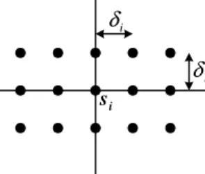
evenly spaced by a distance determined by the value of the probability density function at si. Fig. 1 shows an
example of the synthesized data set for a training sample in a 2-dimensional vector space. The details of the model are elaborated in the following.
i δ i δ i s
Fig. 1. An example of the synthesized data set for a training sample in a 2-dimensional vector space. (i) Samplesiis located at the origin and the neighboring
class-j samples are located at (h1δi, h2δi, …, hmδi), whereh1,h2, …,hmare integers andδiis the average distance between two adjacent class-j training
samples in the proximity of si. How δi is determined will be elaborated later on.
(ii) All the samples in the synthesized data set, including si, have the same function value equal tofj(si). The
value of fj(si) is estimated based on equation (2) in
section 2.
The first phase of the proposed learning algorithm performs an analysis to figure out the values ofwiandσi that make function gi(⋅) defined in the following be a constant function equal tofj(si),
− − =
∑
∞∑
−∞ = ∞ −∞ = 1 2 2 1 2 || ) ,..., ( || exp ) ( h h i i m i i i m h h w g σ δ δ x x L . In other words, gi(x) = fj(si). (3)for all x∈Rm, where R is the set of real numbers. If we take partial derivatives of gi(x1, x2, …, xm), then we will find that
0 ) 0 , , 0 , 0 ( = ∂ ∂ h i x g K and ( 2 , 2 , , 2)=0 ∂ ± ± ± ∂ h i x g δi δi K δi
for all 1≤h≤m. It can be proved in mathematics that local maximums and local minimums of gi(⋅) are located at (a1δi, a2δi, …, amδi) and (( 2) , 1 1 i b + δ (b 2)δi 1 2+ , …, ) ) ( 21 i m
b + δ , where a1, a2, …, amand b1, b2, …, bmare
integers. Therefore, one empirical approach to make equation (3) above satisfied is to find appropriate wiand
σithat make ) ( ) ..., , ( ) 0 ..., , 0 ( i 2 2 j si i g f g = ±δi ±δi = We have − + + =
∑
∑
∞ −∞ = ∞ −∞ = hm i i m h i i h h w g 2 2 2 2 1 2 ) ( exp ) 0 ..., , 0 ( 1 σ δ L L m h i i i h w − =∑
∞ −∞ = 2 2 2 2 exp σ δ , and (4a) ) , , , ( 2i 2i 2i i g −δ −δ L −δ − + + + + =∑ ∑
∞ −∞ = ∞ −∞ = 1 2 2 2 2 1 2 2 1 1 2 ] ) ( ) [( exp h h i i m i m h h w σ δ L L(
)
m h h i i i w − =∑
∞ −∞ = + 2 2 2 2 1 2 ) ( exp σ δ . (4b)Therefore, one of our goals is to findσisuch that
∑
∑
∞ −∞ = ∞ −∞ = − + = − h i i h i i h h 2 2 2 2 1 2 2 2 2 ) ( exp 2 exp σ δ σδ . (5) Let , 8 exp 2 2 − = i i z σδ then we can rewrite equation (5)
as follows:
∑
∑
∞ ∞= + = = + 0 ) 1 2 ( 1 ) 2 ( 2 2 2 2 1 h h h h z z . (6)Since 0 <z< 1, if we want to find the root of equation (6), we can take a limited number of terms from both sides of the equation and find the approximate root. For example, if we take 5 terms from both sides of equation (6), then we have
∑
∑
= + = = + 4 0 ) 1 2 ( 4 1 ) 2 ( 2 2 2 2 1 h h h h zz , which has only one
numerical real root 0.861185. Let z0 = 0.861185.
Then, we have 2 ( ) 0 5 ) 1 2 ( 0 ) 2 ( 0 2 2 > −
∑
∞ = + h h h z z Furthermore, we have∑
∑
∞ = + + ∞ = + = − − − 5 ) 2 2 ( 0 ) 1 2 ( 0 100 0 5 ) 1 2 ( 0 ) 2 ( 0 ) 2 2 ( ) ( 2 2 2 2 2 h h h h h h z z z z z 7 100 0 6.4664 10 2 = × − < z . In summary, we have . 10 4664 . 6 2 2 1 0 7 0 ) 1 2 ( 0 1 ) 2 ( 0 2 2 − ∞ = + ∞ = < × − + <∑
∑
h h h h z zTherefore, z0= 0.861185 is a good approximate root of
equation (6). In fact, we can take more terms from both sides of equation (6) to obtain more accurate approximation.
Given that 0.861185 is a good approximate root of
equation (6) and that
− = 2 2 8 exp i i z σ δ , we need to set σi = 0.91456δi to make equation (5) satisfied. Next, we need to figure out the appropriate value of wi. According to equations (3) and (4a),
we need to setwiso that ) ( 2 exp 2 2 2 i s j m h i i i f h w = −
∑
=∞−∞ σδ or 2 ) ( ) 2925 . 2 ( ) 1 ) 1 ( ) 2925 . 2 ( ) ( 1 m m j m m m j i R n k f w π ⋅ ⋅ ⋅ + ( Γ ⋅ + ≅ = 2 i i s s . (7)The only remaining issue is to determineδi, so that we can compute the value ofσi= 0.91456δiaccordingly. In this paper, we setδito the average distance between two adjacent class-j training samples in the proximity of sample si. In an m-dimensional vector space, the
number of uniformly distributed samples, N, in a hypercube with volume V can be computed byN Vm
α
= ,
whereα is the spacing between two adjacent samples. Therefore, we can computeδiby
m m i k R ) 1 ( ) 1 ( ) ( 2 1+ Γ + = π δ si and obtain . ) 1 ) 1 ( ) ( 6210 . 1 91456 . 0 2 1 m m i i k R + ( Γ + ⋅ = = δ si σ (8)
In equations (7) and (8), parameter m is supposed to be set to the number of attributes of the data set. However, because some attributes of the data set may be correlated, we replace m in equations (7) and (8) by another value, denoted by mˆ in our implementation. The actual value of mˆ is to be determined through cross validation. Actually, the process conducted to figure out optimal mˆ also serves to tune wiandσi in our implementation. Once mˆ is determined, we have the following approximate probability density function for class-j training samples {s1,s2, …,si, …}:
∑
− − = i s i s µ µ 2 2 2 || || exp ) ( ˆ i i j w f σ ( )∑
− − ⋅ = i s i s µ 2 2 ˆ 2 || || exp 50667 . 2 1 1 i m i j n σ σ , (9)whereµis a vector in the m-dimensional vector space, njis the number of class-j training samples, and
m m i k R ˆ 2 ˆ 1 1) ( 1) ( ) ( 6210 . 1 + Γ + ⋅ = si σ .
In fact, because the value of the Gaussian function decreases exponentially, when computing fˆ µj( ) according to equation (9), we only need to include a limited number of nearest training samples of µ. The number of nearest training samples to be included can be determined through cross validation.
As far as the time complexity of the proposed learning algorithm is concerned, for each training sample, we need to identify its k1nearest neighbors of
the same class in the learning phase, where k1 is a
parameter in equation (2). If the kd-tree structure is employed [3], then the time complexity of this process is bounded by O(mn log n + k1n log n), where m is the
number of attributes of the data set and n is total number of training samples. In the classifying phase, we need to identify a fixed number of nearest training samples for each incoming object to be classified. Let k2
denote the fixed number. Then, the time complexity of the classifying phase is bounded by O(mn log n + k2c
log n), where c is the number of objects to be classified. 4. EXPERIMENTAL RESULTS
This section reports the experiments conducted to evaluate the performance of the proposed learning algorithm. Table 1. lists the parameters to be tuned through cross validation in our implementation. In this paper, these parameters are set based on the 10-fold cross validation.
k1 The parameter in equation (2).
k2
The number of nearest training samples included in evaluating the right-hand side of equation (9). mˆ The parameter that substitutes for m in equations (7)
and (8).
Table 1. The parameters to be set through cross validation in the proposed learning algorithm. Tables 2 and 3 compare the accuracy of data classification based on the proposed learning algorithm, the support vector machine, and the KNN classifiers, over 9 data sets from the UCI repository [5]. The collection of benchmark data sets used is the same as that used in [9], except that DNA is not included. DNA is not included, because it contains categorical data and an extension of the proposed learning algorithm is yet to be developed for handling categorical data sets. In Tables 2 and 3, the entry with the highest score in one row is shaded. The parenthesis in the entry
corresponding to the proposed algorithm encloses the values of the three parameters in Table 1. In these experiments, the SVM package used was LIBSVM [6] with the radial basis kernel and the one-against-one practice was conducted.
Table 2 lists the results of the 6 smaller data sets, which contain no separate training and test sets. The number of samples in each of these 6 data sets is listed in the parenthesis below the name of the data set. For these 6 data sets, we adopted the evaluation practice used in [9]. That is, 10-fold cross validation is conducted on the entire data set and the best score is reported. Therefore, the numbers reported just reveal the maximum accuracy that can be achieved, provided that perfect cross validation algorithms are available to identify the optimal parameter values. As Table 2 shows, the data classification based on the proposed learning algorithm and the SVM achieve basically the same level of accuracy for 4 out of these 6 data sets. The two exceptions are glass and vehicle. The benchmark results of these two data sets suggest that both the proposed algorithm and the SVM have some blind spots, and therefore may not be able to perform as well as the other in some cases.
Table 3 provides a more informative comparison, as the data sets are larger and cross validations are conducted to determine the optimal parameter values for the proposed learning algorithm and the SVM. The two numbers in the parenthesis below the name of each data set correspond to the numbers of training samples and test samples, respectively. Again, the results show that the data classification based on the proposed learning algorithm and the SVM generally achieve the same level of accuracy. Tables 2 and 3 also show that the proposed learning algorithm and the SVM generally are able to deliver higher level of accuracy than the KNN classifiers.
In the experiments reported in Tables 2 and 3, no data reduction is performed for the proposed learning algorithm. Table 4 presents the effect of applying a naïve data reduction algorithm. The naïve data reduction algorithm examines the training samples one by one in an arbitrary order. If the training sample being examined and all of its 10 nearest neighbors in the remaining training data set belong to the same class, then the training sample being examined is considered as redundant and is deleted. Since the proposed learning algorithm places one spherical Gaussian function at each training sample, removal of redundant training samples means that the SGF network constructed will contain less nodes and will operate more efficiently. As shown in Table 4, the naïve data reduction algorithm is able to reduce the number of training samples substantially with a minimum impact on classification accuracy, less than 1% on average. The rate of data reduction depends on the characteristics of the data set. For satimage and letter, about one half of the training samples are removed, while over 98% of the training samples in shuttle are considered as redundant. The last row of Table 4 lists the number of
support vectors identified by the SVM software for comparison. One interesting observation is that, for satimage and letter, the numbers of training samples remaining after data reduction is applied and the numbers of support vectors identified by the SVM software are almost equal. For shuttle, the difference is larger. Since the data reduction mechanism employed in this paper is a naïve one, there is room for further improvement with respect to both reduction rate and impact on classification accuracy.
classification algorithms Data sets proposed
algorithm SVM 1NN 3NN 1. iris (150) 97.33 (24, 14, 5) 97.33 94.0 94.67 2. wine (178) 99.44 (3, 16, 1) 99.44 96.08 94.97 3. vowel (528) 99.62 (15, 1, 1) 99.05 99.43 97.16 4. segment (2310) 97.27 (25, 1, 1) 97.40 96.84 95.98 Avg. 1-4 98.42 98.31 96.59 95.70 5. glass (214) 75.74 (9, 3, 2) 71.50 69.65 72.45 6. vehicle (846) 73.53 (13, 8, 2) 86.64 70.45 71.98 Avg. 1-6 90.49 91.89 87.74 87.87
Table 2. Comparison of classification accuracy of the 6 smaller data sets.
classification algorithms Data sets proposed
algorithm SVM 1NN 3NN 7. satimage (4435,2000) 92.30 (6, 26, 1) 91.30 89.35 90.6 8. letter (15000,5000) 97.12 (28, 28, 2) 97.98 95.26 95.46 9. shuttle (43500,14500) 99.94 (18, 1, 3) 99.92 99.91 99.92 Avg. 7-9 96.45 96.40 94.84 95.33
Table 3. Comparison of classification accuracy of the 3 larger data sets.
satimage letter shuttle
# of training samples in the
original data set 4435 15000 43500 # of training samples after
data reduction is applied 1815 7794 627 % of training samples
remaining 40.92% 51.96% 1.44% Classification accuracy
after data reduction is applied
92.15 96.18 99.32
# of support vectors
identified by LIBSVM 1689 8931 287
Table 4. Effects of applying a naïve data reduction mechanism.
Table 5 compares the execution times of carrying out data classification based on the proposed learning algorithm and the SVM. In Table 5, Cross validation
designates the time taken to conduct 10-fold cross validation to figure out optimal parameter values. For SVM, we followed the practice suggested in [9]. In this practice, cross validation is conducted with 225 possible combinations of parameter values. For the proposed learning algorithm, cross validation was conducted over the following ranges for the three parameters listed in Table 1: k1: 1~30; k2: 1~30; mˆ :
1~5.
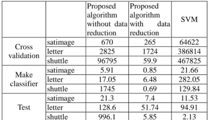
In Table 5, Make classifier designates the time taken to construct a classifier based on the parameter values determined in the cross validation phase. For SVM, this is the time taken to identify support vectors. For the proposed learning algorithm, this is the time taken to construct the SGF networks. Testcorresponds to executing the classification algorithm to label all the objects in the test data set.
Proposed algorithm without data reduction Proposed algorithm with data reduction SVM satimage 670 265 64622 letter 2825 1724 386814 Cross validation shuttle 96795 59.9 467825 satimage 5.91 0.85 21.66 letter 17.05 6.48 282.05 Make classifier shuttle 1745 0.69 129.84 satimage 21.3 7.4 11.53 letter 128.6 51.74 94.91 Test shuttle 996.1 5.85 2.13
Table 5. Comparison of execution times in seconds. As Table 5 reveals, the time taken to conduct cross validation for the SVM classifier is substantially higher than the time taken to conduct cross validation for the proposed learning algorithm. Furthermore, for both SVM and the proposed learning algorithm, once the optimal parameter values are determined, the times taken to construct the classifiers accordingly are insignificant in comparison with the time taken in the cross validation phase. As far as the execution time of the data classification phase is concerned, Table 5 shows that the performance of the SVM and that of the SGF network with data reduction applied are comparable. The actual execution time depends on the number of training samples remaining after data reduction is applied or the number of support vectors.
5. CONCLUSION
In this paper, a novel learning algorithm for constructing data classifiers with RBF networks is proposed. The main distinction of the proposed learning algorithm is the way it exploits local distributions of the training samples in determining the optimal parameter values of the basis functions. The experiments presented in this paper reveal that data classification with the proposed learning algorithm generally achieves the same level of accuracy as the support vector machines. One important advantage of the proposed data classification
algorithm, in comparison with the support vector machine, is that the process conducted to construct a RBF network with the proposed learning algorithm normally takes much less time than the process conducted to construct a SVM. As far as the efficiency of the classifier is concerned, the naïve data reduction mechanism employed in this paper is able to reduce the size of the training data set substantially with a minimum impact on classification accuracy. One interesting observation in this regard is that, for all three data sets used in data reduction experiments, the number of training samples remaining after data reduction is applied is quite close to the number of support vectors identified by the SVM software.
As the study presented in this paper looks quite promising, several issues deserve further study. The first issue is the development of advanced data reduction mechanisms for the proposed learning algorithm. Advanced data reduction mechanisms should be able to deliver higher reduction rates than the naïve mechanism employed in this paper without sacrificing classification accuracy. The second issue is the extension of the proposed learning algorithm for handling categorical data sets. The third issue concerns why the proposed learning algorithm fails to deliver comparable accuracy in the vehicle test case, what the blind spot is, and how improvements can be made.
6. APPENDIX Assume that
1
2
1 s sk
sˆ ,ˆ ,...,ˆ are the k1 nearest training
samples of sithat belongs to the same class as si. If k1is
sufficiently large and the distribution of these k1samples
in the vector space is uniform then we have
) 1 ( ) ( 2 1 2 + Γ ≈ m m m R k ρ si π , whereρis the local density of samples
1
2
1 s sk
sˆ ,ˆ ,...,ˆ in the proximity of si. Furthermore, we have
∫
∑
− ≈ Γ( 2 − = ) ( 0 1 1 ) 2 || ˆ || 2 1 i m s R m m k h rdr r π ρ i h s s ) ( ) 1 ( ) ( 2 2 1 2 m m m R m Γ + = ρ si +π , where ) ( 2 2 1 2 m m m r Γ −πis the surface area of a hypersphere with radius r in an m-dimensional vector space. Therefore, we have
∑
= − ⋅ + = 1 1 1 || ˆ || 1 1 ) ( k h k m m R si sh si .The right-hand side of the equation above is then employed in this paper to estimate R(si).
7. REFERENCES
[1] E. Artin, The Gamma Function, New York, Holt, Rinehart, and Winston, 1964.
[2] F. Belloir, A. Fache, and A. Billat, "A general approach to construct RBF net-based classifier,"
Proceedings of the 7th European Symposium on Artificial Neural Network, pp. 399-404, 1999. [3] J. L. Bentley, "Multidimensional binary search
trees used for associative searching," Communication of the ACM, vol. 18, no. 9, pp. 509-517, 1975.
[4] M. Bianchini, P. Frasconi, and M. Gori, "Learning without local minima in radial basis function networks," IEEE Transaction on Neural Networks, vol. 6, no. 3, pp. 749-756, 1995.
[5] C. L. Blake and C. J. Merz, "UCI repository of bmachine learning databases," Technical report, University of California, Department of Information and Computer Science, Irvine, CA, 1998.
[6] C. C. Chang and C. J. Lin, "LIBSVM: a library for support vector machines," http://www.csie.ntu. edu.tw/~cjlin/libsvm, 2001.
[7] N. Cristianini and J. Shawe-Taylor, An Introduction to Support Vector Machines, Cambridge University Press, Cambridge, UK, 2000.
[8] S. Dumais, J. Platt, and D. Heckerman, "Inductive learning algorithms and representations for text categorization," Proceedings of the International Conference on Information and Knowledge Management, pp. 148-154, 1998.
[9] C. W. Hsu and C. J. Lin, "A comparison of methods for multi-class support vector machines," IEEE Transactions on Neural Networks, vol. 13, pp. 415-425, 2002.
[10] Y. S. Hwang and S. Y. Bang, "An efficient method to construct a radial basis function neural network classifier," Neural Networks, vol. 10, no. 8, pp. 1495-1503, 1997.
[11] T. Joachims, "Text categorization with support vector machines: learning with many relevant features," Proceedings of European Conference on Machine Learning, pp. 137-142, 1998.
[12] V. Kecman, Learning and Soft Computing: Support Vector Machines, Neural Networks, and Fuzzy Logic Models, The MIT Press, Cambridge, Massachusetts, London, England, 2001.
[13] M. J. L. Orr, "Introduction to radial basis function networks," Technical report, Center for Cognitive Science, University of Edinburgh, 1996.
[14] A. Papoulis, Probability, Random Variables, and Stochastic Processes, McGraw-Hill, 1991.
[15] B. Scholkopf, K. K. Sung, C. Burges, F. Girosi, P. Niyogi, T. Poggio, and V. Vapnik, "Comparing support vector machines with gaussian kernels to radial basis function classifiers," IEEE Transactions on Signal Processing, vol. 45, no. 11, pp. 1-8, 1997.