Robust H-infinity output feedback control for general nonlinear systems with structured uncertainty

This article was downloaded by: [National Chiao Tung University 國立交通大學] On: 27 April 2014, At: 02:33

Publisher: Taylor & Francis

Informa Ltd Registered in England and Wales Registered Number: 1072954 Registered office: Mortimer House, 37-41 Mortimer Street, London W1T 3JH, UK

Journal of the Chinese Institute of Engineers

Publication details, including instructions for authors and subscription information: http://www.tandfonline.com/loi/tcie20

Robust H

output feedback control for general

nonlinear systems with structured uncertainty

a

Department of Electronic Engineering , Hwa Hsia Institute of Technology , Taipei, Taiwan, 235, R.O.C. Phone: 886–2–89415128; Fax: 886–2–89415128; E-mail:

b

Department of Electrical and Control Engineering , National Chiao Tung University , Hsinchu, Taiwan, 300, R.O.C.

Published online: 04 Mar 2011.

To cite this article: Jenq‐Lang Wu & Tsu‐Tian Lee (2004) Robust H 8

output feedback control for general nonlinear systems with structured uncertainty, Journal of the Chinese Institute of Engineers, 27:7, 1069-1075, DOI:

10.1080/02533839.2004.9670962

To link to this article: http://dx.doi.org/10.1080/02533839.2004.9670962

PLEASE SCROLL DOWN FOR ARTICLE

Taylor & Francis makes every effort to ensure the accuracy of all the information (the “Content”) contained in the publications on our platform. However, Taylor & Francis, our agents, and our licensors make no

representations or warranties whatsoever as to the accuracy, completeness, or suitability for any purpose of the Content. Any opinions and views expressed in this publication are the opinions and views of the authors, and are not the views of or endorsed by Taylor & Francis. The accuracy of the Content should not be relied upon and should be independently verified with primary sources of information. Taylor and Francis shall not be liable for any losses, actions, claims, proceedings, demands, costs, expenses, damages, and other liabilities whatsoever or howsoever caused arising directly or indirectly in connection with, in relation to or arising out of the use of the Content.

This article may be used for research, teaching, and private study purposes. Any substantial or systematic reproduction, redistribution, reselling, loan, sub-licensing, systematic supply, or distribution in any

form to anyone is expressly forbidden. Terms & Conditions of access and use can be found at http:// www.tandfonline.com/page/terms-and-conditions

Short Paper

ROBUST

H

OUTPUT FEEDBACK CONTROL FOR GENERAL

NONLINEAR SYSTEMS WITH STRUCTURED UNCERTAINTY

Jenq-Lang Wu* and Tsu-Tian Lee

ABSTRACT

In this paper, the robust H∞ output feedback control problem for general nonlinear systems with L2-norm-bounded structured uncertainties is considered. Sufficient

con-ditions for the solvability of robust performance synthesis problems are represented in terms of two Hamilton-Jacobi inequalities with n independent variables. Based on these conditions, a state space characterization of a robust H∞ output feedback con-troller solving the considered problem is proposed. An example is provided for illus-tration.

Key Words: H∞ control, nonlinear systems, robust performance, structured uncertainty.

*Corresponding author. (Tel: 89415128; Fax: 886-2-86683945; Email: wujl@cc.hwh.edu.tw)

J. L. Wu is with the Department of Electronic Engineering, Hwa Hsia Institute of Technology, Taipei, Taiwan 235, R.O.C.

T. T. Lee is with the Department of Electrical and Control Engi-neering, National Chiao Tung University, Hsinchu, Taiwan 300, R.O.C.

I. INTRODUCTION

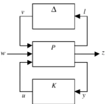
In this paper, the robust H∞ output feedback con-trol problem for continuous-time general nonlinear systems with structured uncertainty will be consid-ered. The block diagram of the considered problem is shown in Fig. 1, where P is the normal system, which is nonlinear and time-invariant, and ∆ is the structured uncertainty. The design objective is to find an output feedback controller, K, such that the closed-loop system is internally stable and its L2-gain from

w to z is less than, or equal to, some positive number, γ, for all possible structured uncertainties ∆.

In the case of no uncertainty, ∆, in the system, the problem becomes the well-known nonlinear H∞ control problem, see, e.g., (Ball et al., 1993; Isidori and Astolfi, 1992; Isidori, 1994; Isidori and Kang, 1995; Isidori and Lin, 1998; Lu and Doyle, 1994; Van der Schaft, 1991; 1992; and Yung et al., 1996; 1998). It has been shown that the solution to the nonlinear

H∞ output feedback control problem can be obtained by solving two Hamilton-Jacobi equations (or

inequalities), which are the nonlinear versions of the Riccati equations considered in the corresponding lin-ear H∞ control theory, see, e.g., (Doyle et al., 1989). However, the H∞ control problem for nonlinear systems with structured uncertainty is more difficult. The robust H∞ control problem for linear systems with structured uncertainty has been considered in (Doyle, 1982; Lu et al., 1996; and Poola and Tikku, 1995). The studies of nonlinear H∞ control problems with structured uncertainty are few. The only result is a state-space characterization of robustness analysis and synthesis for affine nonlinear systems provided by Lu and Doyle (1997). Specifically, sufficient conditions for the solvability of robustness synthesis problem are represented in terms of scaling Nonlinear Matrix Inequalities (NLMIs). However, in (Lu and Doyle, 1997), the considered system is assumed to be affine in control input and external input. Moreover, only the state feedback case is considered. In this paper, we first extend the results of the robust H∞ state feed-back control problem for affine nonlinear systems in (Lu and Doyle, 1997) to the case of general nonaffine nonlinear systems. Furthermore, not only state feed-back but also output feedfeed-back cases are considered in this paper. Sufficient conditions for the solvabil-ity of robust H∞ output feedback control problems for general nonlinear systems with structured uncertainty are represented in terms of two Hamilton-Jacobi in-equalities with n independent variables. Finally, based

1070 Journal of the Chiness Institute of Engineers, Vol. 27, No. 7 (2004)

on these conditions, a state space characterization of an output feedback controller solving the considered problem is provided.

In what follows, x 2 denotes xT_{x; x}

M 2

denotes

xT_{Mx; P}

L₂ denotes the L2-norm of the system P;

M>0 means that the matrix M is positive definite; M<0 means that the matrix M is negative definite.

II. PROBLEM FORMULATION

Consider a smooth uncertain nonlinear system shown in Fig. 1. The normal plant P is described by the following dynamic equations

P: x = F(x, w, v, u) y = Y(x, w, v, u) z = Z(x, w, v, u) li= Li(x, w, v, u), i = 1, 2, , N (1)

where x∈Rn _{represents the state, u}∈_Rm _{is the control}

input, and w∈Rr _{represents a set of exogenous inputs,} z∈Rs _{is the controlled variable, and y}∈_Rp _{is the}

meas-ured variable. Without losing of generality, assume that F(0,0,0,0)=0, Z(0,0,0,0)=0, Y(0,0,0,0)=0, and

Li(0,0,0,0)=0 for all i=1, 2, ..., N.

The uncertainty is described as

vi=∆i(li), i=1, 2, ..., N (2)

where

∆i∈B∆∆i≡{∆i|∆i is causal and asymptotically

stable for li=0, and has L2-gain≤ρi}

with ρi>0. Or equivalently, v=∆(l) where l=[l₁T l₂T ... l_NT]T , v=[v1T v2T ... vNT] T , and ∆∈∆∆≡{∆=diag{∆1, ∆2, ..., ∆N}|∆i∈B∆∆i}

Suppose li∈Rni and vi∈Rmi, i=1, 2, ..., N. Let m =

mi

Σ

N

.

The design objective is to construct an output feedback controller which will asymptotically stabi-lize the resulting closed-loop system locally and render its L2-gain (from w to z) less than or equal to γ

for all ∆∈∆∆.

Suppose that the state of ∆i is ςςi. Let ςς≡[ςς1 T _ςς

2 T

... _ςς

N

T]ΤΤΤΤΤ_{. As in (Lu and Doyle, 1997), the following}

assumption is made.

Assumption (A1). For each i∈{1, 2, ..., N}, ∆i has a

unique asymptotically stable equilibrium at ςςi=0 for li=0; in addition, there is a differentiable storage

func-tion Ui(ςςi) such that

dUi(ςςi(t)) dt ≤ρi2 li(t) 2 – vi(t) 2 +ϕϕi(ςςi(t)) , (3)

with some negative definite function ϕi(.). III. STATE FEEDBACK CASE

In this section, we will focus on the robust H∞ state feedback control problem for system (1). De-fine a Hamiltonian function H1: Rn×Rn×Rr×R

m ×Rm→ R as H1(x, p1, w, v, u) = p₁T_{F(x, w, v, u) + Z(x, w, v, u)} 2_–γ2 _w 2 + [ρi2 Li(x, w, v, u) 2 – vi 2

Σ

Suppose plant (1) satisfies the following assumption.

Assumption (A2). The matrix D₁₃TD₁₃ is positive

defi-nite, and D11 T D11–γ2I D11 T D12 D12 T D11 D12 T D12– I is negative defi-nite.

Fig. 1 Block diagram of the considered system

Assumption (A2) guarantees the existence and uniqueness of solutions w*(x, p1), v*(x, p1), and u*(x,

p1), defined in the neighborhood of (x, p1)=(0, 0),

satisfying ∂H1 ∂w (x, p1, w*(x, p1), v*(x, p1), u*(x, p1))=0 ∂H1 ∂v (x, p1, w*(x, p1), v*(x, p1), u*(x, p1))=0 ∂H1 ∂u (x, p1, w*(x, p1), v*(x, p1), u*(x, p1))=0 with w*(0, 0)=0, v*(0, 0)=0, u*(0, 0)=0

This can be drawn from the implicit function theo-rem.

Moreover, suppose the system (1) satisfies the “detectability” assumption given below.

Assumption (A3). Any bounded trajectory x(t) of the

system x(t)=F(x(t), 0, v(t), u(t)) satisfying Z(x(t), 0,

v(t), u(t))=0 for all t≥0, is such that lim_{t→ ∞}x(t)=0.

Then, the following result holds.

Theorem 1. Consider system (1). Suppose

Assump-tions (A1), (A2), and (A3) hold. Suppose the fol-lowing hypothesis also holds.

(H1) There exists a smooth, positive definite func-tion V(x), locally defined in the neighborhood of x=0, such that the function

Y1(x) = H1(x, Vx T (x)), w*(x, Vx T (x)), v*(x, Vx T (x)), u_*(x, V_xT(x)) (6)

is negative semidefinite near x=0, where Vx(x)

denotes the row vector ∂V/∂x1 ∂V/∂x2 ... ∂V/

∂xn.

Then the system (1) with the feedback law u=u*(x,

VxT(x)) is locally internally stable and has L2-gain

(from w to z) less than or equal to γ for all ∆∈∆∆.

Proof of Theorem 1: For simplicity of notation, we

denote w*(x)=w*(x, Vx T (x)), v*(x)=v*(x, Vx T (x)) and u*(x)=u*(x, Vx T (x)). Let p≡[wT vT uT ]T . Using the Taylor expansion theorem and noting (4) and (6), we have H1(x, VxT(x), w, v, u) = Y1(x) + w – w*(x) v – v*(x) u – u*(x) _R(x) 2 + o w – w*(x) v – v*(x) u – u*(x) 3 where R(x) = r₁₁(x) r₁₂(x) r₁₃(x) r₂₁(x) r₂₂(x) r₂₃(x) r₃₁(x) r₃₂(x) r₃₃(x) ≡1 2 ∂2 H1(x, Vx T (x), w, v, u) ∂p2 w = w*(x), v = v*(x), u = u*(x)

It is easy to show that

R(0) = D11 T D11–γ2I D11 T D12 D11 T D13 D12 T D11 D12 T D12– I D12 T D13 D13 T D11 D13 T D12 D13 T D13

which is nonsingular by Assumption (A2).

Consider the candidate storage function U(x, ςς) =V(x)+

Σ

i = 1 N

, which is positive definite. Setting

u=u*(x) in (1) yields a closed-loop system satisfying

dU dt + Z(x, w, v, u*(x)) 2 –γ2 _w 2 ≤Y1(x) + w – w*(x) v – v*(x) T r11(x) r12(x) r21(x) r22(x) w – w*(x) v – v*(x) + o w – w_{v – v}*(x) *(x) 3 +

Σ

Then, from hypothesis (H1) and Assumptions (A1) and (A2), we immediately have the following dissi-pation inequality

dU

dt + Z(x, w, v, u*(x)) 2

–γ2 _w 2≤₀

in the neighborhood of the origin. Thus, the closed-loop system has L2–gain≤γ. It remains to prove that

the closed-loop system is locally asymptotically sta-ble. To this end, letting w=0 in (7), it yields

dU dt ≤– Z(x, 0, v, u*(x)) 2 + Y1(x) + – w*(x) v – v*(x) T _r 11(x) r12(x) r21(x) r22(x) – w*(x) v – v*(x) + o – w*(x) v – v*(x) 3 +

Σ

which is negative semidefinite near the origin by hypothesis (H1) and Assumptions (A1) and (A2). This proves that the equilibrium x_ςς =0 of the closed-loop system is stable. To prove the asymptotic stability of the closed-loop system, note that equation (8) implies

1072 Journal of the Chiness Institute of Engineers, Vol. 27, No. 7 (2004) dU dt ≤– Z(x, 0, v, u*(x)) 2 +

Σ

IV. OUTPUT FEEDBACK CASE

The major contribution of this paper is to pro-pose an output feedback controller

ξξ=F(ξξ, u*(ξξ), v*(ξξ), w*(ξξ))

+G(ξξ)(y–Y(ξξ, u*(ξξ), v*(ξξ), w*(ξξ)))

u=u*(ξξ) (10)

to solve the considered robust H∞ control problem, where ξξ∈Rn

is defined in the neighborhood of the ori-gin, and the output injection gain G(ξξ) is a matrix to be determined.

For convenience, the corresponding closed-loop system is expressed as

xo=Fo (xo , w, v) y=Yo (xo , w, v) z=Zo (xo , w, v) li=Li o (xo , w, v) vi=∆i(li), i=1, 2, ..., N where xo = x_ξξ , Fo (xo , w, v)= F(x, w, v, u*(ξξ)) F(x,ξξ, w, v) Yo (xo , w, v)=Y(x, w, v, u*(ξξ)) Zo (xo , w, v)=Z(x, w, v, u*(ξξ)) L_io(xo , w, v)=Li(x, w, v, u*(ξξ)) and F(x,ξξ, w, v)=F(ξξ, w*(ξξ), v*(ξξ), u*(ξξ)) +G(ξξ)(Y(x, w, v, u*(ξξ)) –Y(ξξ, w*(ξξ), v*(ξξ), u*(ξξ)))

In what follows, we shall show how to

asymptotically stabilize the closed-loop system lo-cally and render its L2–gain≤γ (from w to z) for all

∆∈∆∆.

Define a Hamiltonian function H2: R2n×R2n×Rr×

Rm_{→R as} H2(xo, p2, w, v) = p2TF o (xo_{, w, v) +} w – w*(x) v – v*(x) u*(ξξ) – u*(x) T ⋅ (1 –(1 –εε11)r)r1121(x) (1 –(x) (1 –εε11)r)r2212(x)(x) rr2313(x)(x) r31(x) r32(x) (1 +ε3)r33(x) ⋅ w – wv – v**(x)(x) u*(ξξ) – u*(x) (11)

where 0<ε1<1 and ε3>0. Then, by implict function

theorem, there exist unique smooth functions w(xo_, p2) and v(xo, p2), defined in the neighborhood of (xo,

p2)=(0, 0), satisfying ∂H2(xo, p2, w, v) ∂w _{w = w(x}o_{, p} 2), v = v(xo, p2) = 0 ∂H2(xo, p2, w, v) ∂v w = w(xo_{, p} 2), v = v(xo, p2) = 0 with w(0, 0) = 0 and v(0, 0) = 0.

As a result, we have the following theorem.

Theorem 2. Consider system (1). Suppose

Assump-tions (A1), (A2) and (A3), and hypothesis (H1) in Theo-rem 1 hold. Suppose the following hypothesis also holds. (H2) There exists a smooth real-valued function

M(xo_{), which is locally defined in the}

neighbor-hood of xo_{=0, and which vanishes at x=}ξξ _{and is}

positive elsewhere, such that the function

Y2(xo) = H2(xo, MxTo(xo), w(xo, M_xTo(xo)) ,

v(xo_{, M} xo

T_(xo₎₎₎

vanishes at x=ξξ and is negative elsewhere. Then the system (1) with the output feedback controller (10) is locally internally stable and has L2

-gain (from w to z) less than or equal to γ for all ∆∈∆∆. Proof of Theorem 2: Using the Taylor expansion

theorem yields

H2(xo, MxTo(xo), w, v) = Y2(xo) + w – w(xo_{, M} xo T (xo₎₎ v – v(xo_{, M} xTo(xo)) R2(xo) 2 + o w – w(x o_{, M} xTo(xo)) v – v(xo_{, M} xTo(xo)) 3 (12) where R2(xo) = 1 2 ∂2 H2 ∂w2 ∂2 H2 ∂v∂w ∂2 H2 ∂w∂v ∂ 2 H2 ∂v2 w = w(xo_{, M} xTo(xo_{)), v = v(x}o_{, M} xo T_(xo₎₎

which is negative definite near the origin. Consider the candidate storage function

Uo(xo_,ςς_{) = M(x}o_{) + V(x) + U} i(ςςi)

Σ

i = 1 N

which is positive for all x

o

ςς ≠0. Along the

trajecto-ries of the closed-loop system, we have

dUo dt + Z(x, w, v, u*(ξξ)) 2 –γ2 _w 2 ≤Y₁(x) + Y₂(xo_{) +} ϕ i(ςςi)

Σ

in the neighborhood of the origin. Then, we can prove this Theorem via a procedure similar to the proof of Theorem 1. So, the detailed proof is omitted here for saving space.

The function Y2(xo) thus obtained has 2n

independent variables and actually involves the undeter-mined matrix G(ξξ). In what follows, we shall show how to reduce the number of independent variables in Y2(xo),

and how to determine the output injection gain G(ξξ). To this end, define a Hamiltonian function H3:

Rn× Rn× Rp× Rr×_Rm→ R as H3(x, p3, p4, w, v) = p3TF(x, w, v, 0) – p4TY(x, w, v, 0) + w – w*(x) v – v*(x) – u*(x) T ⋅ (1 –(1 –εε11)r)r1121(x) (1 –(x) (1 –εε11)r)r2212(x)(x) rr2313(x)(x) r31(x) r32(x) (1 +ε3)r33(x) ⋅ w – wv – v**(x)(x) – u*(x) (14)

and suppose the plant (1) satisfies the following ad-ditional assumption.

Assumption (A4). The measurement output Y(x, w, v, u) is such that the matrix D21=[Yw(0, 0, 0, 0) Yv(0,

0, 0, 0)] has full row rank.

Then, by implict function, theorem there exist unique smooth functions w(x, p₃, p₄) and v(x, p3, p4),

defined in the neighborhood of (x, p3, p4)=(0,0,0),

sat-isfying ∂H₃(x, p₃, p₄, w, v) ∂w _{w = w(x, p} 3, p4), v = v(x, p3, p4) = 0 w(0, 0, 0) = 0 ∂H3(x, p3, p4, w, v) ∂v _{w = w(x, p} 3, p4), v = v(x, p3, p4) = 0 v(0, 0, 0) = 0

Moreover, it is easy to verify that

∂2 H3(x, p3, p4, w(x, p3, p4), v(x, p3, p4)) ∂p42 _{(x, p} 3, p4) = (0, 0, 0) = 1 2(1 –ε1) D21 r11(0) r12(0) r21(0) r22(0) – 1 D21 T < 0

which is nonsingular. Thus, there exists a smooth function p4*(x, p3), defined in the neighborhood of

(0,0) such that

∂H3(x, p3, p4, w(x, p3, p4), v(x, p3, p4))

∂p4 _p

4= p4*(x, p3)

=0 p4*(0, 0)=0

Then, we have the following result.

1074 Journal of the Chiness Institute of Engineers, Vol. 27, No. 7 (2004)

Theorem 3. Consider system (1). Suppose

Assump-tions (A1), (A2), and (A3), and hypothesis (H1) in Theo-rem 1 hold. Suppose the following hypothesis also holds. (H3) There exists a smooth, positive definite func-tion Q(x), locally defined in the neighborhood of the origin in Rn

, such that the function

Y3(x) = H3(x, QxT(x), p4*(x, QxT(x)) ,

w(x, QxT(x), p4*(x, QxT(x))),

v(x, Q_xT(x), p_4*(x, Q_xT(x)))) (15) is negative definite near x=0, and its Hessian matrix is nonsingular at x=0. If the equation

Qx(x)G(x) = p4*(x, Qx T

(x)) (16)

has a smooth solution G(x), then the system (1) with the output feedback controller (10) is locally inter-nally stable and has L2-gain (from w to z) less than or

equal to γ for all ∆∈∆∆.

Proof of Theorem 3: It suffices to prove that M(xo

)≡Q(x–ξξξξξ) with Qx(x)G(x)=p4*(x, Qx T

(x)) which satisfies hypothesis (H2). Clearly, M(xo

)≡Q(x–ξξξξξ) vanishes at x=ξξξξξ and is positive elsewhere. Set

Y2(xo) = H2(xo, MTxo(xo), w(xo, M_xTo(xo)), v(xo_{, M} xTo(xo))) where M(xo )=Q(x–ξξξξξ) and Qx(x)G(x)=p4*(x, Qx T (x)). It remains to prove that Y2(x

o

) vanishes at x=ξξ and is negative elsewhere. This can be proven via a similar procedure as that presented in (Yung et al., 1998). Therefore, it is omitted for saving the space.

V. EXAMPLE

Consider a system (denoted by system P) which has the following realization

x1= 4x1x2– 2x13– x13x22+ x2w – 2x1x2v1+ x1u2 x2= – 14x2– 5x23+ 3₄x12x2– v2+ 2(1 + x12)u y = 20 3x1+ 5x1x2+ 2x13x2+ w z = x12+ u l1= x22 l2= x12 v1=∆1(l1) v2=∆2(l2)

where the uncertain terms ∆1 and ∆2 satisfy ||∆1||L₂≤3

and ||∆2||L₂≤1. Suppose Assumption (A1) holds. Here

we want to find a state feedback controller and an output feedback controller, respectively, such that the closed loop system is internally stable and has L2–

gain≤1 (form w to z) for all possible ∆1 and ∆2.

State Feedback Case:

For system P, it is easy to verify that Assump-tion (A2) holds. From Theorem 1, it can be shown that the positive definite function

V(x) = 1

2x12+ x22

satisfies Hypothesis (H1). The corresponding Y1(x) is

Y1(x) = – 31x22– x24–

9x12x22

4 –

x14

1 + x12

which is negative definite for all x≠0. The worst-case disturbance w is

w = w*(x) = 1₂x1x2

Moreover, if we choose the state feedback controller as

u = u*(x) = –

x12

1 + x12

– 2x2

then the closed-loop system will be internally stable and its L2–gain (from w to z) will be less than or equal

to 1.

Output Feedback Case:

For output feedback, it can be shown that As-sumption (A4) holds. Moreover, the positive defi-nite function Q(x)=x12+ 1₂x22 satisfies Hypothesis (H3)

with ε1=ε3= 1 2. The corresponding Y3(X) is Y3(x) = ( 3 1 + x12 – 4)x14– 3₄x22– 5x24– 5₂x12x22 – x12(20₃ + 5x2+ 2x12x2) 2

which is negative definite near x=0. Moreover,

p4*(x) = 40₃x1+ 12x1x2+ 4x13x2

Let the output injection gain G(x)= G1(x)

G2(x) . Since Qx(x)G(x)=p4*(x) i.e. [2x₁ x₂]⋅ G1(x) G₂(x) = 403x1+ 12x1x2+ 4x13x2

has a smooth solution

G1(x)

G₂(x) = 20

3 + 6x2

4x₁3

So the output feedback H∞ control problem is solv-able. Moreover, with the output feedback controller

ξ1= 4ξ1ξ2– 2ξ1 3 +ξ1 3_ξ 2 2 + 1 2ξ1ξ2 2 +ξ1( ξ1 2 1 +ξ1 2+ 2ξ2) 2 + (20 3 + 6ξ2)⋅(y – 20₃ξ1– 11₂ξ1ξ2– 2ξ1 3_ξ 2) ξ2= – 13ξ2– 5ξ2 3_{+ 3} 4ξ1 2_ξ 2– 2(ξ1 2_{+ 2(1 +ξ} 1 2_)ξ 2) + 4ξ1 3 (y – 20 3ξ1– 11₂ξ1ξ2– 2ξ1 3_ξ 2) u = – ξ1 2 1 +ξ1 2 – 2ξ2

the closed-loop system will be internally stable and its

L2-gain (from w to z) will be less than or equal to 1.

VI. CONCLUSIONS

In this paper, a state-space characterization of robust H∞ output feedback controllers for general nonlinear systems with L2-gain-bounded structured

uncertainties has been proposed. Sufficient condi-tions for the solvability of robust performance syn-thesis problems have been represented in terms of two Hamilton-Jacobi inequalities with n independent vari-ables. Based on these conditions, an output feedback

H∞ controller solving the considered problem has been provided. The example shows that the provided method is useful.

ACKNOWLEDGMENTS

This work was supported in part by National Science Council, Taiwan, Republic of China under Grant NSC-89-2213-E-146-008.

REFERENCES

Ball, J. A., Helton, J. W., and Walker, M. L., 1993, “H∞ Control for Nonlinear Systems with Output Feedback,” IEEE Transations on Automatic

Con-trol, Vol. 38, No. 4, pp. 546-559.

Doyle, J., 1982, “Analysis of Feedback Systems with Structured Uncertainties,” IEE Proceedings, Part D, Vol. 129, No. 6, pp. 242-250.

Doyle, J. C., Glover, K., Khargonekar, P. P., and Francis, B. A., 1989, “State-Space Solutions to Standard H2

and H∞ Control Problems,” IEEE

Transations on Automatic Control, Vol. 34, No.

8, pp. 831-846.

Isidori, A., 1994, “H∞ Control via Measurement Feed-back for Affine Nonlinear Systems,”

Interna-tional Journal of Robust and Nonlinear Control,

Vol. 4, No. 4, pp. 553-574.

Isidori, A., and Astolfi, A., 1992, “Disturbance At-tenuation and H∞-Control via Measurement Feed-back in Nonlinear Systems,” IEEE Transations

on Automatic Control, Vol. 37, No. 9, pp.

1283-1293.

Isidori, A., and Kang, W., 1995, “H∞ Control via Measurement Feedback for General Nonlinear Systems,” IEEE Transations on Automatic

Con-trol, Vol. 40, No. 3, pp. 466-472.

Isidori, A., and Lin, W., 1998, “Global L2-Gain State

Feedback Design for a Class of Nonlinear Sys-tems,” Systems & Control Letters, Vol. 34, No. 5, pp. 295-302.

Lu, W. M., and Doyle, J. C., 1994, “H∞ Control of Nonlinear System via Output Feedback: Con-troliers Parametrization,” IEEE Transations on

Automatic Control, Vol. 39, No. 12, pp. 2517-2521.

Lu, W. M., and Doyle, J. C., 1997, “Robustness Analysis and Synthesis for Nonlinear Uncertain Systems,” IEEE Transations on Automatic

Con-trol, Vol. 42, No. 12, pp. 1654-1662.

Lu, W. M., Zhou, K., and Doyle, J. C., 1996, “Stabilization of Uncertain Linear Systems: An LFT Approach,” IEEE Transations on Automatic

Control, Vol. 41, No. 1, pp. 51-65.

Poolla, K., and Tikku, A., 1995, “Robust ance Against Time-Varying Structured Perform-ances,” IEEE Transations on Automatic Control, Vol. 40, No. 9, pp. 1589-1601.

Van der Schaft, A. J., 1991. On a State Space Approach to Nonlinear H∞ Control, Systems & Control Letters, Vol. 16, No. 1, pp. 1-8.

Van der Schaft, A. J., 1992, “L2

-Gain Analysis of Nonlinear Systems and Nonlinear State Feedback

H∞ Control,” IEEE Transations on Automatic

Control, Vol. 37, No. 6, pp. 770-784.

Yung, C. F., Lin, Y. P., and Yeh, F. B., 1996, “A Family of Nonlinear H∞ Output Feedback trollers,” IEEE Transations on Automatic

Con-trol, Vol. 41, No. 2, pp. 232-236.

Yung, C. F., Wu, J. L., and Lee, T. T., 1998, “H∞ Control for More General Nonlinear Systems,”

IEEE Transations on Automatic Control, Vol. 43,

No. 12, pp. 1724-1727.

Manuscript Received: Jul. 01, 2003 Revision Received: Oct. 07, 2003 and Accepted: Dec. 12, 2003