使用星狀骨架作人類動作自動辨識

全文

(1)使用星狀骨架作人類動作自動辨識研究生：陳宣勝. 指導教授：李素瑛. 國立交通大學資訊工程研究所. 摘要. 這篇論文提出一建構在隱藏式馬可夫模型的動作辨識方法，此方法使用星狀骨架來對人類的姿勢做出代表性的描述。星狀骨架是一種藉由連結物件中心到物件輪廓突出點的快速骨架技巧。為了使用星狀骨架作為動作辨識的特徵，我們明確地定義星狀骨架如何作為辨識的特徵。因為頭和四肢經常是人形狀的突出點，所以辨識的特徵被定義為星狀的五維向量。此辨識方法將人的動作視為沿著時間的一連串星狀骨架，因此，表示人類動作的時間序列影像被轉換成特徵向量序列。接著，特徵向量序列必須轉換成符號序列使得隱藏式馬可夫模型可以為動作建立模型。我們設計一本包含每一類動作星狀骨架的姿勢編碼書並且為特徵向量定義距離來量測特徵向量間的相似度。姿勢序列中的每個特徵向量會和編碼書中的特徵向量做比對，並會被編碼成編碼書中與自己最為相似的特徵向量所代表的符號。因此時間序列的姿勢影像被轉換成符號序列。我們以隱藏式馬可夫模型為每種被辨識的動作建立模型。在訓練模型的階段，每個動作模型的參數皆最佳化以適當地描述訓練的符號序列。在動作辨識的階段，與測試符號序列最相配的動作模型即為所辨識出的動作。 i.

(2) 我們建立一個可以自動地辨識出十種不同動作的系統，這個系統分成兩種情況對人類動作影片作測試。第一種情況是我們對一百個包含單一動作的影片作分類，此系統達到了百分之九十八的辨識率。另一種是比較實際的情況，由一個人做出一連串不同的動作，系統即時的辨識出目前的動作。實驗的結果顯現出大有可為的效果。. 檢索詞：動作辨識、星狀骨架、隱藏式馬可夫模型循序樣式. ii.

(3) Human Action Recognition Using Star Skeleton Student: Hsuan-Sheng Chen. Advisor: Suh-Yin Lee. Institute of Computer Science and Information Engineering National Chiao-Tung University. Abstract. This paper presents a HMM-based methodology for action recognition using star skeleton as a representative descriptor of human posture. Star skeleton is a fast skeletonization technique by connecting from centroid of target object to contour extremes. To use star skeleton as feature for action recognition, we clearly define the feature as a five-dimensional vector in star fashion because the head and four limbs are usually local extremes of human shape. In our proposed method, an action is composed of a series of star skeletons over time. Therefore, time-sequential images expressing human action are transformed into a feature vector sequence. Then the feature vector sequence must be transformed into symbol sequence so that HMM can model the action. We design a posture codebook, which contains representative star skeletons of each action type and define a star distance to measure the similarity between feature vectors. Each feature vector of the sequence is matched against the codebook and is assigned to the symbol that is most similar. Consequently, the. iii.

(4) time-sequential images are converted to a symbol posture sequence. We use HMMs to model each action types to be recognized. In the training phase, the model parameters of the HMM of each category are optimized so as to best describe the training symbol sequences. For human action recognition, the model which best matches the observed symbol sequence is selected as the recognized category. We implement a system to automatically recognize ten different types of actions, and the system has been tested on real human action videos in two cases. One case is the classification of 100 video clips, each containing a single action type. A 98% recognition rate is obtained. The other case is a more realistic situation in which human takes a series of actions combined. An action-series recognition is achieved by referring a period of posture history using a sliding window scheme. The experimental results show promising performance.. Index Terms: Action recognition, star skeleton, star distance, HMM. iv.

(5) Acknowledgment I greatly appreciate the kind guidance of my advisor, Prof. Suh-Yin Lee. Without her graceful suggestion and encouragement, I cannot complete this thesis. Besides I want to give my thanks to all the members in the Information System Laboratory for their suggestion and instruction, especially Mr. Hua-Tsung Chen, Mr. Yi-Wen Chen and Mr. Ming-Ho Hsiao. Finally I would like to express my appreciation to my parents. This thesis is dedicated to them.. v.

(6) Table of Contents Abstract (Chinese) ........................................................................................................i Abstract (English) ...................................................................................................... iii Acknowledgement ........................................................................................................v Table of Contents ........................................................................................................vi List of Figures.............................................................................................................vii List of Tables............................................................................................................. viii Chapter 1 Introduction................................................................................................1 Chapter 2 Hidden Markov Model (HMM)................................................................5 2.1 Elements of an HMM.......................................................................................6 2.2 Recognition Process Of HMM.........................................................................8 2.3 Learning Process Of HMM............................................................................11 Chapter 3 Proposed Action Recognition Method....................................................16 3.1 System Overview ...........................................................................................16 3.2 Feature Extraction..........................................................................................18 3.3 Feature Definition ..........................................................................................19 3.3.1 Star Skeletonization ............................................................................19 3.3.2 Feature Definition ...............................................................................21 3.4 Mapping features to symbols .........................................................................21 3.4.1 Vector Quantization ............................................................................22 3.4.2 Star Distance .......................................................................................23 3.5 Action Recognition ........................................................................................23 3.6 Action Series Recognition..............................................................................24 Chapter 4 Experimental Results and discussions ...................................................26 4.1 Single action recognition ...............................................................................26 4.2 Recognition over a series of actions ..............................................................31 Chapter 5 Conclusions and Future Works .....................................................36 vi.

(7) List of Figures Figure 2-1 HMM Concept.............................................................................................7 Figure 2-2 Illustration of the forward algorithm .........................................................10 Figure 2-3 The induction step of the forward algorithm.............................................11 Figure 2-4 Illustration of the sequence of operations required for the computation of the backward variable β t (i ) .........................................................................................13 Figure 2-5 Illustration of the sequence of operations required for the computation of the joint event that the system is in state S i at time t and state S j at time t+1...............14 Figure 3-1 Illustration of the system architecture .......................................................17 Figure 3-2 A walk action is a series of postures over time .........................................18 Figure 3-3 Process flow of star skeletonization ..........................................................20 Figure 3-4 The concept of vector quantization in action recognition .........................22 Figure 3-5 Illustration of star distance (a) Mismatch (b) Greedy Match ....................23 Figure 3-6 Sliding-window scheme for action series recognition ..............................25 Figure 4-1 Example clips of each action type.............................................................28 Figure 4-2 Features of each action type using star skeleton .......................................30 Figure 4-3 Complete recognition process of sit action ...............................................30 Figure 4-4 Recognition over a series of actions ‘sit up – jump2 – walk – crawl1’ ....33 Figure 4-5 Recognition over a series of actions ‘sidewalk – walk – pickup’ .............34 Figure 4-6 Recognition over a series of actions ‘crawl 2 – walk – jump 2’ ...............35. vii.

(8) List of Tables Table 1 Confusion matrix for recognition of testing data ...........................................31. viii.

(9) Chapter 1 Introduction. Vision-based human motion recognition is currently one of the most active research areas in the domain of computer vision. It is motivated by a great deal of applications, such as automated surveillance system, smart home application, video indexing and browsing, virtual reality, human-computer interface and analysis of sports events. Unlike gesture and sign language, there is no rigid syntax and well-defined structure that can be used for action recognition. This makes human activity recognition a more challenging task. Several human action recognition methods were proposed in the past few years. A detailed survey can be found in [1, 2]. Most of the previous methods can be classified into two classes: model-based methods [3, 4, 5] and training-based learning methods [6-24]. It is natural to think that human recognized action using the structure of human posture. The fundamental strategy of model-based methods achieves human action recognition by using estimated or recovered human posture. Hogg [3] recovered pedestrian’s posture from a monocular camera by using a cylinder model. Wren et al. [4] estimated human pose by using a color based body parts tracking technique. In [5], a learning-based method for recovering 3D human body pose from single images and monocular image sequences is presented. Recovering human posture is an efficient method for motion recognition since the human action and its posture are highly related. However, a large amount of computation cost is required for pose estimation. An eigenspace technique [6] is one of the learning based recognition techniques and it is also used in the action recognition field [7]. An action given by successive 1.

(10) video frames is expressed as a curve (called a motion curve) in an eigenspace, and, by adopting a similarity measure, it can be used in judging if an unknown action is similar to any of the memorized motion curves. In [8], two kinds of superposed images are used to represent a human action: a motion history image (MHI) and a superposed motion image (SMI). Employing these images, a human action is described in an eigenspace as a set of points, and each SMI plays a role of reference point. An unknown action image is transformed into the MHI and then a match is found with images described in the eigenspace to realize action recognition. The eigenspace technique achieves high speed human action recognition. However, the recognition rate is not good enough. Hidden Markov Model (HMM) which has been used successfully in speech recognition is also one of the learning based recognition techniques, and Yamato et al. [17] are the first researchers who applied it for action recognition. They use HMM to recognize six different tennis strokes among three players. Some of the recent works [18, 19, 20, 21, 22, 23, 24] have shown that HMM performs well in human action recognition as well. A HMM is built for each action. Given an unknown human action sequence, features are extracted and then mapped into symbols. The action recognition is done by choosing the maximal likelihood from the trained HMM action models. Human actions can be viewed as continuous sequences of discrete postures, including key postures and transitional postures. Key postures uniquely belong to one action so that people can recognize the action from a single key posture. Transitional postures are interim between two actions, and even human cannot recognize the action from a single transitional posture. Therefore, human action can not be recognized from a single frame. Due to robustness, rich mathematical structure and great capability in dealing with time-sequential data, HMM is chosen as the technique 2.

(11) for action recognition. To recognize human action, features must be extracted. Shape information is an important clue to represent postures since we regard an action as a sequence of discrete postures. Width [18] or horizontal and vertical histograms [21] of the binary shapes associated to humans are too rough to represent the shape information due to great loss of data. On the other hand, it is not efficient to use the whole human silhouettes. Although Principle Component Analysis (PCA) can be used to reduce the redundancy [9, 22], the computational cost is high due to matrix operations. To find a good balance of the tradeoff, we must best describe the distribution of human shape with minimal expenses. Since a posture can be deemed as silhouettes of a torso and protruding limbs, a star skeleton technique [26], which is built by connecting the center of human body to protruding limbs, is adopted to best describe the shape information. In our proposed algorithm, time-sequential images expressing human action are transformed to an image feature vector sequence by extracting a feature vector from each image. Each feature vector of the sequence is assigned a symbol which corresponds to a codeword in the codebook created by Vector Quantization [27]. Consequently, the time-sequential images are converted to a symbol sequence. In the learning phase, the model parameters of the HMM of each category are optimized so as to best describe the training symbol sequences from the categories of human action to be recognized. For human recognition, the model which best matches the observed symbol sequence is selected as the recognized category. The paper is organized as follows. In chapter 2, we introduce the concept of HMM and how to use it for recognition. In chapter 3 we present the proposed algorithm with a detailed description of each step and some examples. Then experimental results and discussion are reported in chapter 4. Finally conclusion and 3.

(12) future work are outlined in chapter 5.. 4.

(13) Chapter 2 Hidden Markov Model. Real-world processes generally produce observable outputs which can be characterized as signals. The signals can be discrete in nature (e.g., characters from a finite alphabet, quantized vectors from a codebook, etc.), or continuous in nature (e.g., speech samples, temperature measurements, music, etc.). A problem of fundamental interest is characterizing such real-world signals in terms of signal models. There are several reasons why one is interested in applying signal models. First of all, a signal model can provide the basis for a theoretical description of a signal processing system which can be used to process the signal so as to provide a desired output. A second reason why signal models are important is that they are potentially providing us a great deal of information about the signal source without having to have the source available. Finally, the most important reason is that they often work extremely well in practice, and can be realized into important practical systems － e.g. prediction systems, recognition systems, identification systems, etc., in a very efficient manner. There are several possible choices for signal models to characterize the properties of a given signal source. Broadly one can dichotomize the types of signal models into the class of deterministic models, and the class of statistical models. Deterministic models generally exploit some known specific properties of the signal, e.g., the signal is a sine wave, or a sum of exponentials, etc. In these cases, specification of the signal model is generally straightforward; all that is required is to determine (estimate) the values of the parameters of the signal model (e.g., amplitude, frequency, phase of a sine wave, amplitudes and rates of exponentials). The second 5.

(14) broad class of signal models is the set of statistical properties of the signal. Examples of such statistical models include Gaussian processes, Poisson processes, Markov processes, and hidden Markov processes, among others. The underlying assumption of the statistical model is that the signal can be well characterized as a parametric random process, and that the parameters of the stochastic process can be determined or estimated in a precise, well-defined manner. Since an action is composed of postures, it can be viewed as a signal by mapping a distinct posture to a symbol or vector. Therefore a signal model can be applied to describe an action. We compute the probabilities (or likelihood) that the observed signal (action) was produced by each signal (action) model. Recognition can be done by choosing the model which best matches the observations. Because of the great success in speech recognition and fine mathematical structure, HMM is used to model an action.. 2.1 Elements of an HMM An HMM consists of a number of states each of which is assigned a probability of transition from one state to another state. With time, state transitions occur stochastically. Like Markov models, states at any time depend only on the state at the preceding time. One symbol is yielded from one of the HMM states according to the probabilities assigned to the states. HMM states are not directly observable, and can be observed only through a sequence of observed symbols. To describe a discrete HMM, the following notations are defined. T = length of the observation sequence. Q = {q1 , q 2 , L , q N } : the set of states. N = the number of states in the model. V = {v1 , v 2 , L , v M } : the set of possible output symbols. 6.

(15) M = the number of observation symbols. A = {aij | aij = Pr ( st +1 = q j | st = qi )} : state transition probability, where. aij is the probability of transiting from state qi to state q j . B = {b j (k ) | b j (k ) = Pr (v k | st = q j )} : symbol output probability, where. b j (k ) is the probability of output symbol v k at state q j . π = {π i | π i = Pr ( s1 = qi )} initial state probability.. λ = { A, B, π } Complete parameter set of the model Using this model, transitions are described as follows:. S = {st }, t = 1, 2, L , T : State s t is the t th state (unobservable). O = O1 , O2 , L , OT : Observed symbol sequence (length = T ).. a31. a11. a13. a22 a12. a23. a21. a32. b1(1) b1(2) b1(3). v1. v2. v3. b2(1) b2(2) b2(3). v1. v2. a33. b3(1) b3(2) b3(3). v3. v1. v2. v3. Hidden ( non − observable). Observed Symbol Sequencee. O1 , O2 , O3 , O4 , O5 , K OT Time t. Figure 2-1 HMM Concept. 7.

(16) Figure 2-1 illustrates the concept of a HMM with a transition graph. There are. three states in this example indicated as circles. Each directed line is a transition from one state to another, where the transition probability from state qi to state q j is indicated by the character aij alongside the line. Note that there are also transition paths from states to themselves. These paths can provide the HMM with time-scale invariability because they allow the HMM to stay in the same state for any duration. Each state of the HMM stochastically outputs a symbol. In state q j , symbol v k is output with a probability of b j (k ) . If there are M kinds of symbols, b j (k ) become N×M matrix. The HMM output the symbol sequence O = O1 , O2 , K , OT from time 1 to T. We can observe the symbol sequences output by the HMM but we can not observe the HMM states. The initial state of the HMM is also determined stochastically by the initial state probability π . A HMM is characterized by three matrices: state transit probability matrix A, symbol output probability matrix B, and initial state probability matrix π . The parameters of A, B, and π are determined during the learning process described in section 2.3. As described in section 2.2, one HMM is created for each category to be recognized. Recognizing time-sequential symbols is equivalent to determining which HMM produced the observed symbol sequence. In section 2.2 and 2.3, the recognition and learning procedures are explained respectively.. 2.2 Recognition Process Of HMM To recognize observed symbol sequences, we create one HMM for each category. For. 8.

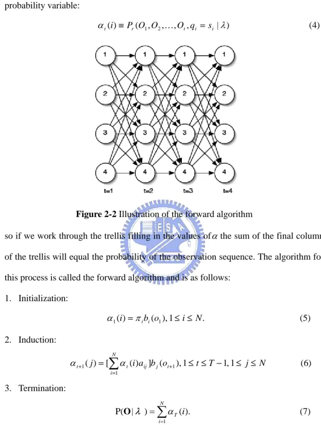
(17) a classifier of C categories, we choose the model which best matches the observations from C HMMs, where λi = { Ai , Bi , π i }, i = 1, 2,L, C. This means that when a sequence of unknown category is given, we calculate Pr (λ i | O), O = O1O2 K OT for each HMM λ i and select λ co , where c o = arg max ( Pr (λ i | O)) i. Given the observation sequence O = O1O2 K OT and the HMM λ i , i = 1, 2, L, C . According to the Bayes rule, the problem is how to evaluate Pr (O | λ i ) , the probability that the sequence was generated by HMM λ i .. The probability of the observations O for a specific state sequence Q is: T. P( O | Q, λ ) = ∏ P(ot | qt , λ ) = bq1 (o1 ) × bq 2 (o2 ) LbqT (oT ). (1). t =1. and the probability of the state sequence is: P (Q | λ ) = π q1 a q1q 2 a q 2 q 3 L a qT −1qT. (2). so we can calculate the probability of the observations given the model as:. P (Q | λ ) = ∑ P(O | Q, λ ) P(Q | λ ) = Q. ∑π. b (o1 )a q1q 2 bq1 (o2 ) L a qT −1qT bqT (oT ) (3). q1 q1. q1LqT. This result allows the evaluation of the probability of O, but to evaluate it directly would be exponential in T.. A better approach is to recognize that many redundant calculations would be made by directly evaluating equation 3, and therefore caching calculations can lead to reduced complexity. We implement the cache as a trellis of states at each time step, calculating the cached valued (called α ) for each state as a sum over all states at the previous time step. α is the probability of the partial observation sequence o1 , o2 L ot and 9.

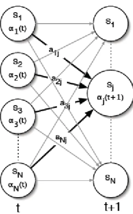
(18) state si at time t. This can be visualized as in Figure 2-2. We define the forward probability variable:. α t (i) ≡ Pr (O1 , O2 ,K, Ot , qi = si | λ ). (4). Figure 2-2 Illustration of the forward algorithm. so if we work through the trellis filling in the values of α the sum of the final column of the trellis will equal the probability of the observation sequence. The algorithm for this process is called the forward algorithm and is as follows: 1. Initialization:. α 1 (i) = π i bi (o1 ), 1 ≤ i ≤ N .. (5). 2. Induction: N. α t +1 ( j ) = [∑ α t (i )aij ]b j (ot +1 ), 1 ≤ t ≤ T − 1, 1 ≤ j ≤ N. (6). i =1. 3. Termination: N. P(O | λ ) = ∑ α T (i ).. (7). i =1. The induction step is the key to the forward algorithm and is depicted in Figure 2-3. For each state s j , α j (t ) stores the probability of arriving in that state having. observed the observation sequence up until time t.. 10.

(19) Figure 2-3 The induction step of the forward algorithm. We can calculate the likelihood of each HMM using the above equation and select the most likely HMM as the recognition result.. 2.3 Learning Process Of HMM The most difficult problem of HMMs is to determine a method to adjust the model parameters ( A, B, π ) to maximize the probability of the observation sequence given the model. There is no known way to analytically solve for the model which maximizes the probability of the observation sequence. In fact, given any finite observation sequence as training data, there is no optimal way of estimating the model parameters. We can, however, choose λ = ( A, B, π ) such that P (O | λ ) is locally maximized using an iterative procedure such as the Baum-Welch method.. 11.

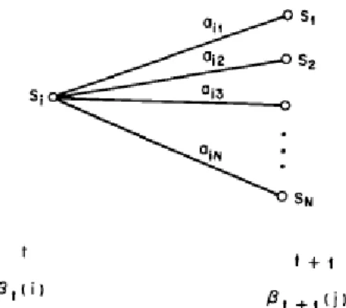
(20) In the learning phase, each HMM must be trained so that it is most likely to generate the symbol patterns for its category. Training an HMM means optimizing the model parameters ( A, B, π ). to. maximize. the. probability. of. the. observation. sequence Pr (O | λ ) . The Baum-Welch algorithm is used for these estimations. Define:. β t (i) ≡ P(Ot +1 ,K, OT | st = qi , λ ) , i.e., the probability of the partial observation sequence from t+1 to the end, given state S i at time t and the model λ .. β t (i) is called the backward variable and can also be solved inductively in a manner similar to that used for the forward variable α t (i ) , as follows: (1) Initialization:. β T (i ) = 1, 1 ≤ i ≤ N. (8). (2) Induction: N. β t (i ) = ∑ aij b j (Ot +1 )β t +1 ( j ), t = T − 1, T − 2, L , 1, 1 ≤ i ≤ N .. (9). j =1. The initialization step (1) arbitrary defines β T (i ) to be 1 for all i. Step (2), which is illustrated in Figure 2-4, shows that in order to have been in state S i at time t, and to account for the observation sequence from time t+1 on, you have to consider all possible states S j at time t+1, accounting for the transition from S i to S j (the aij term), as well as the observation Ot +1 in state j (the b j (Ot +1 ) term), and then account for the remaining partial observation sequence from state j ( the β t +1 (i ) term).. 12.

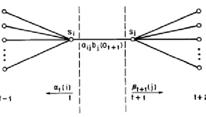
(21) Figure 2-4 Illustration of the sequence of operations required for the computation of the backward variable β t (i ). We define the variable. γ t (i) ≡ P( st = qi | O1 , K, OT , λ ) α (i) β t (i) = t . P(O | λ ). (10). i.e., the probability of being in state S i at time t, given the observation sequence O, and the model λ .. In order to describe the procedure for re-estimation (iterative update and improvement) of HMM parameters, we first define ε t (i, j ) , the probability of being in state S i at time t, and state S j at time t+1, given the model and the observation sequence, i.e.. ε t (i, j ) ≡ P(qt = si , qt +1 = q j | O, λ ).. (11). The sequence of events leading to the conditions required by (10) is illustrated in Figure 2-5. It should be clear, from the definitions of the forward and backward. variables, that we can write ε t (i, j ) in the form. ε t (i, j ) = =. α t (i)aij b j (Ot +1 ) β t +1 ( j ) P(O | λ ) α t (i )aij b j (Ot +1 ) β t +1 ( j ) N. N. ∑ ∑ α (i)a b (O i =1 j =1. t. ij. j. t +1. (12). ) β t +1 ( j ). where the numerator term is just P (qt = S i , qt +1 = S j , O | λ ) and the division 13.

(22) by P(O | λ ) gives the desired probability measure.. Figure 2-5 Illustration of the sequence of operations required for the computation of. the joint event that the system is in state S i at time t and state S j at time t+1 We have previously defined γ t (i ) as the probability of being in state S i at time t, given the observation sequence and the model; hence we can relate γ t (i ) to ε t (i, j ) by summing over j, giving N. γ t (i ) = ∑ ε t (i, j ).. (13). j =1. If we sum γ t (i ) over the time index t, we get a quantity which can be interpreted as the expected (over time) number of times that state S i is visited, or equivalently, the expected number of transitions made from state S i (if we exclude the time slot t = T from the summation). Similarly, summation of ε t (i, j ) over t (from t = 1 to t = T-1) can be interpreted as the expected number of transitions from state S i to state S j . That is T −1. ∑γ t =1. t. (i ) = expected number of transitions from S i .. (14). t. (i, j ) = expected number of transitions from S i to S j .. (15). T −1. ∑ε t =1. Using the above formulas (and the concept of counting event occurrences) we can give a method for re-estimation of the parameters of an HMM. A set of reasonable. 14.

(23) re-estimation formulas for π , A, and B are. π i = expected frequency (number of times) in state S i at time(t = 1) = γ 1 (i ) . aij =. (16). exp ected number of transitions from state S i to state S j exp ected number of transitions from state S i T −1. =. ∑ε t =1 T −1. ∑γ t =1. b j (k ) =. (17). (i, j ). t. t. (i ). exp ected number of times in state j and observing symbol v k exp ected number of times in state j T. ∑γ t =1. =. t. ( j). (18). s .t . Ot = vk T. ∑γ t =1. t. ( j). If we define the current model as λ = ( A, B, π ) , and use that to compute the right hand sides of (16)-(18), and we define the re-estimated model as λ = ( A , B , π ) , as determined from the left-hand sides of (16)-(18), then it has been proven by Baum and his colleagues that either (1) the initial model λ defines a critical point of the likelihood function, in which case λ = λ ; or (2) model λ is more likely than model λ in the sense that P (O | λ ) ⟩ P (O | λ ) , i.e. we have found a new model λ from which the observation sequence is more likely to have been produced. Based on the above procedure, if we iteratively use λ in place of λ and repeat the re-estimation calculation, we then can improve the probability of O being observed from the model until some limiting point is reached. The final result of this re-estimation procedure is called a maximum likelihood estimate of the HMM.. 15.

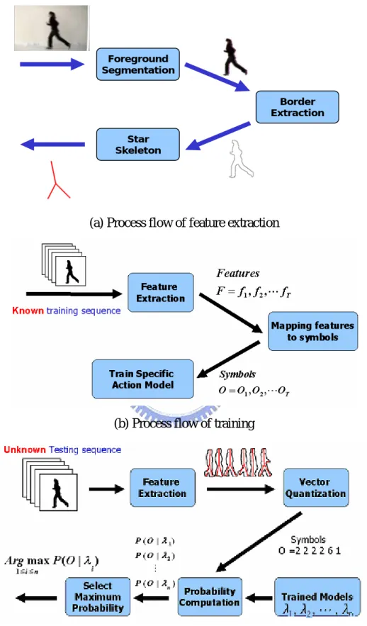
(24) Chapter 3 Proposed Action Recognition Algorithm 3.1 System Overview The system architecture consists of three parts, including feature extraction, mapping features to symbols and action recognition as shown in Figure 3-1. For feature extraction, we use background subtraction and threshold the difference between current frame and background image to segment the foreground object. After the foreground segmentation, we extract the posture contour from the human silhouette. As the last phase of feature extraction, a star skeleton technique is applied to describe the posture contour. The extracted star skeletons are denoted as feature vectors for latter action recognition. The process flow of feature extraction is shown in Figure 3-1 (a). After the feature extraction, Vector Quantization (VQ) is used to map feature vectors to symbol sequence. We build a posture codebook which contains representative feature vectors of each action, and each feature vector in the codebook is assigned to a symbol codeword. An extracted feature vector is mapped to the symbol which is the codeword of the most similar (minimal distance) feature vector in the codebook. The output of mapping features to symbols module is thus a sequence of posture symbols. The action recognition module involves two phase: training and recognition. We use Hidden Markov Models to model different actions by training which optimizes model parameters for training data. Recognition is achieved by probability computation and selection of maximum probability. The process flows of both training and recognition are shown in Figure 3-1 (b) and (c).. 16.

(25) Foreground Segmentation Border Extraction Star Skeleton. (a) Process flow of feature extraction. (b) Process flow of training. (c) Process flow of recognition Figure 3-1 Illustration of the system architecture. 17.

(26) Figure 3-2 A walk action is a series of postures over time. 3.2 Feature Extraction Human action is composed of a series of postures over time as shown in Figure 3-2. A good way to represent a posture is to use its boundary shape. However, using the whole human contour to describe a human posture is inefficient since each border point is very similar to its neighbor points. Though techniques like Principle Component Analysis are used to reduce the redundancy, it is computational expensive due to matrix operations. On the other hand, simple information like human width and height may be rough to represent a posture. Consequently, representative features must be extracted to describe a posture. Human skeleton seems to be a good choice. There are many standard techniques for skeletonization such as thinning and distance transformation. However, these techniques are computationally expensive and moreover, are highly susceptible to noise in the target boundary. Therefore, a simple, real-time, robust techniques, called star skeleton [26] was used as features of our action recognition scheme.. 18.

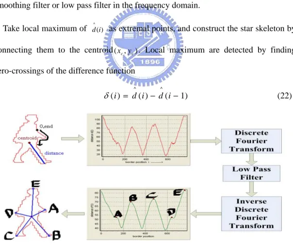
(27) 3.3 Feature Definition Vectors from the centroid of human body to local maximas are defined as the feature vector, called star vector. The head, two hands, and two legs are usually outstanding parts of extracted human contour, hence they can properly characterize the shape information. As they are usually local maximas of the star skeleton, we define the dimension of the feature vector five. For postures such as the two legs overlap or one hand is covered, the number of protruding portion is below five. Zero vectors are added. In the same way, we can adjust the low-pass filter to reduce the number of local maximas for postures with more than five notable parts.. 3.3.1 Star Skeletonization The concept of star skeleton is to connect from centroid to gross extremities of a human contour. To find the gross extremities of human contour, the distances from the centroid to each border point are processed in a clockwise or counter-clockwise order. Extremities can be located in representative local maximum of the distance function. Since noise increases the difficulty of locating gross extremes, the distance signal must be smoothed by using smoothing filter or low pass filter in the frequency domain. Local maximum are detected by finding zero-crossings of the smoothed difference function. The star skeleton is constructed by connecting these points to the target centroid. The star skeleton process flow of an example human contour is shown in Figure 4 and points A, B, C, D and E are local maximum of the distance function. The details of star skeleton are as follows: Star skeleton Algorithm(As described in [26]) Input: Human contour Output: A skeleton in star fashion. 19.

(28) 1. Determine the centroid of the target image border ( x c , y c ) Nb. xc =. 1 Nb. ∑x. yc =. 1 Nb. Nb. i =1. ∑y i =1. i. (19). i. (20). where N b is the number of border pixels, and ( xc , y c ) is a pixel on the border of the target. 2. Calculate the distances d i from the centroid ( xc , y c ) to each border point ( xi , yi ) d i = ( xi − x c ) 2 + ( y i − y c ) 2. (21). These are expressed as a one dimensional discrete function d (i) = d i . ^. 3. Smooth the distance signal d (i ) to d (i ) for noise reduction by using linear smoothing filter or low pass filter in the frequency domain. ^. 4. Take local maximum of d (i ) as extremal points, and construct the star skeleton by connecting them to the centroid ( xc , y c ) . Local maximum are detected by finding zero-crossings of the difference function ^. ^. δ ( i ) = d ( i ) − d ( i − 1). Figure 3-3 Process flow of star skeletonization. 20. (22).

(29) 3.3.2 Feature Definition One technique often used to analyze the action or gait of human is the motion of skeletal components. Therefore, we may want to find which part of body (e.g. head, hands, legs, etc) the five local maximum represent. In [26], angles between two legs are used to distinguish walk from run. However, some assumptions such as feet locate on lower extremes of star skeleton are made. These assumptions can not fit other different actions, for example, low extremes of crawl may be hands. Moreover, the number of extremal points of star skeleton varies with human shape and the low pass filter used. Gross extremes are not necessarily certain part of human body. Because of the difficulty in finding which part of body the five local maximum represent, we just use the distribution of star skeleton as features for action recognition. As a feature, the dimension of the star skeleton must be fixed. The feature vector is then defined as a five dimensional vectors from centroid to shape extremes because head, two hands, two legs are usually local maximum. For postures with more than five contour extremes, we adjust the low pass filter to lower the dimension of star skeleton to five. On the other hand, zero vectors are added for postures with less than five extremes. Since the used feature is vector, its absolute value varies for people with different size and shape, normalization must be made to get relative distribution of the feature vector. This can be achieved by dividing vectors on x-coordinate by human width, vectors on y-coordinate by human height.. 3.4 Mapping features to symbols To apply HMM to time-sequential video, the extracted feature sequence must be transformed into symbol sequence for latter action recognition. This is accomplished by a well-known technique, called Vector Quantization [27]. 21.

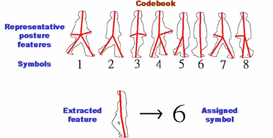
(30) 3.4.1 Vector Quantization. For vector quantization, codewords g j ∈ R n , which represent the centers of the clusters in the feature R n space, are needed. Codeword g j is assigned to symbol v j . Consequently, the size of the code book equals the number of HMM output. symbols. Each feature vector f i is transformed into the symbol which is assigned to the codeword nearest to the vector in the feature space. This means f i is transformed into symbol v j if j = arg min j d ( f i , g j ) where d ( x, y ) is the distance between vectors x and y.. Figure 3-4 The concept of vector quantization in action recognition. For action recognition, we select m feature vectors of representative postures from each action as codewords in the codebook. And an extracted feature would be mapped to a symbol, which is the codeword of the most similar (minimal distance) feature vector in the codebook. The concept of the mapping process is shown in Figure 3-4. The codebook in the figure contains only some representative star skeletons of walk to explain the mapping concept. In the mapping process, similarity between feature vectors needs to be determined. Therefore we define distance between feature vectors, called star distance, to decide the similarity between feature vectors.. 22.

(31) 3.4.2 Star Distance. Since the star skeleton is a five-dimensional vector, the star distance between two feature vectors S and T is first defined as the sum of the Euclidean distances of the five sub-vectors. 5. Dis tan ce = ∑ (S i − Ti ). (23). i =1. However, consider the star skeletons S and T in Figure 3-5 (a). The two star skeletons are similar, but the distance between them is large due to mismatch. So we modify the distance measurement. Each sub-vector must find their closest mapping as shown in Figure 3-5 (b). The star distance is then defined as the sum of the Euclidean distance. of the five sub-vectors under such greedy mapping. For simplicity, the star distance is obtained by minimal sum of the five sub-vectors in all permutation. Better algorithm to accelerate the star distance calculation can be found. 5!. 5. k =1. i =1. Star Distance = Arg min ∑ (Si − Ti ). (a). (24). (b). Figure 3-5 Illustration of star distance (a) Mismatch (b) Greedy Match. 3.5 Action Recognition The idea behind using the HMMs is to construct a model for each of the actions that we want to recognize. HMMs give a state based representation for each action. The number of states was empirieally determined. After training each action model, we calculate the probability P (O | λ i ) , the probability of model λ i generating the 23.

(32) observation posture sequence O, for each action model. We can then recognize the action as being the one, which is represented by the most probable model.. 3.6 Action Series Recognition What mentioned above are classification of single action. The following is a more complex situation. A man performs a series of actions, and we recognize what action he is performing now. One may want to recognize the action by classification of the posture at current time T. However, there is a problem. By observation we can classify postures into two classes, including key postures and transitional postures. Key postures uniquely belong to one action so that people can recognize the action from a single key posture. Transitional postures are interim between two actions, and even human cannot recognize the action from a single transitional posture. Therefore, human action can not be recognized from posture of a single frame due to transitional postures. So, we refer a period of posture history to find the action human is performing. A sliding-window scheme is applied for real-time action recognition as shown in Figure 7. At time current T, symbol subsequence between T-W and T, which is a period of posture history, is used to recognize the current action by computing the maximal likelihood, where W is the window size. In our implementation, W is set to thirty frames which is the average gait cycle of testing sequences. Here we recognize stand as walk. The unknown is due to not enough history. By the sliding window scheme, what action a man is performing can be realized.. 24.

(33) Figure 3-6. Sliding-window scheme for action series recognition. 25.

(34) Chapter 4 Experiment Results and Discussion To test the performance of our approach, we implement a system capable of recognizing ten different actions. The system contains two parts: (1) Single Action Recognition (2) Recognition over a series of actions. In (1), a confusion matrix was used to present the recognition result. In (2), we compare the real-time recognition result to ground truth obtained by human.. 4.1 Single action recognition The proposed action recognition system has been tested on real human action videos. For simplicity, we assumed a uniform background in order to extract human regions with less difficulty. The categories to be recognized were ten types of human actions: ‘walk’, ‘sidewalk‘, ‘pickup’, ‘sit’, ‘jump 1’, ‘jump 2’, ‘push up’, ‘sit up’, ‘crawl 1’, and ‘crawl 2’. 5 persons performed each type of the 10 actions 3 times. The video content was captured by a TV camera (NTSC, 30 frames / second) and digitized into 352x240 pixel resolution. The duration of each video clip was from 40 to 110 frames. This number of frames is chosen experimentally: shorter sequences do not allow to characterize the action and, on the other side, longer sequences make the learning phase very hard. Figure 4-1 showed some example video clips of the 10 types of human actions. In order to calculate the recognition rate, we used the leave out method. All data were separated into 3 categories, each category containing 5 persons doing ten different actions one time. One category was used as training data for building a HMM for each action type, and the others were testing data.. 26.

(35) (a) walk. (b) sidewalk. (c) sit. (d) pick up. (e) jump 1. (f) jump2. (g) push up. 27.

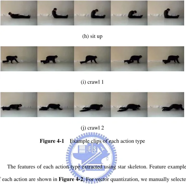
(36) (h) sit up. (i) crawl 1. (j) crawl 2 Figure 4-1 Example clips of each action type. The features of each action type extracted using star skeleton. Feature examples of each action are shown in Figure 4-2. For vector quantization, we manually selected m representative skeleton features for each action as codewords in the codebook for the experiment. In my implementation, for simple actions like sidewalk and jump2, m is set to five. Other eight actions m is set to ten. Thus, the total number of HMM symbols was 90. We build the codebook in one direct first and reverse all the features vectors for recognition of counter actions.. (a) walk. 28.

(37) (b) sidewalk. (c) sit. (d) pick up. (e) jump 1. (f) jump 2. (g) push up. (h) sit up. (i) crawl 1. (j) crawl 2 29.

(38) Figure 4-2 Features of each action type using star skeleton. We use a sit action video to explain the recognition process. The sit action is composed of a series or postures. Star skeleton are used for posture description, and map the sit action into feature sequence. The feature sequence is then transformed into symbol sequence O by Vector Quantization. Each trained action model compute the probability generating symbol sequence O, the log scale of probability are shown in Figure 4-3. The sit model has the max probability, so the video are recognized as sit.. Figure 4-3 Complete recognition process of sit action. 30.

(39) Table 1. Confusion matrix for recognition of testing data. Finally, Table 1 demonstrated the confusion matrix of recognition of testing data. The left side is the ground truth action type, the upper side is the recognition action type. The number on the diagonal is the number of each action which are correctly classified. The number which are not on the diagonal are misunderstand, and we can see which kind of action the system misjudge. From this table, we can see that most of the testing data were accurately classified. A great recognition rate of 98% was achieved by the proposed method. Only two confusions occurred only between sit and pick up. We check the two mistaken clips, they contain large portion of bending the body. And the bending does not uniquely belong to sit or pickup so that the two action models confuse. In my opinion, a transitional action, bending, must be added to better distinguish pickup and sit.. 4.2 Recognition over a series of actions In the experiment, human take a series of different actions, and the system will automatic recognize the action type in each frame. 3 different action series video clips are used to test the proposed system. We compare the recognition result to human-made ground truth to evaluate the system performance.. 31.

(40) The first test sequence is “Sit up – get up – Jump 2 – turn about – Walk – turn about – Crawl 1”. The second test sequence is “Sidewalk – turn about – Walk – turn about – Pick up”. The third test sequence is “Crawl 2 – get up – turn about – Walk – turn about – Jump2”. Each sequence contains about 3-4 defined action types and 1-2 undefined action types (transitional action). Figure 4-4, 4-5, 4-6 (a) shows the original image sequence (some selected frames) of the four action series respectively. The proposed system recognized the action type by the sliding window scheme. Figure 4-4, 4-5, 4-6 (b) shows the recognition result. The x-coordinate of the graph is. the frame number, and the y-coordinate indicates the recognized action. The red line is the ground truth defined by human observation, and the blue line is the recognized action types. The unknown period is the time human performs actions that are not defined in the ten categories. The first period of unknown of ground truth is get up, and the second and third period are turn about. The unknown period of recognition result is due to the history of postures is not enough (smaller than the window size). By these graphs, we can see that the time human perform the defined actions can be correctly recognized. Some misunderstanding can be corrected by smoothing the recognition signal. A small recognition time delay occurs at the start of crawl due to not enough history for the sliding window scheme. However, the delay is very small that human can hardly feel. The time period human perform undefined action, the system choose the most possible action from ten defined actions. Therefore, more different actions must be added to enhance the system.. 32.

(41) (a) Some original image sequences of ‘sit up – jump2 – walk – crawl1’. 10. Recognition result. 9. Ground Truth. 8 0. unknown. 1. walk. 2. sidewalk. 3. sit. 4. 4. pickup. 3. 5. jump1. 2. 6. jump2. 1. 7. push up. 0. 8. sit up. 9. crawl 1. 10. crawl 2. action type. 7 6 5. 1. 47 93 139 185 231 277 323 369 415 461 507 553 frame number. (b) Recognition result Figure 4-4 Recognition over a series of actions ‘sit up – jump2 – walk – crawl1’. 33.

(42) (a) Some original image sequences of ‘sidewalk – walk – pickup’. 10. Recognition result. 9. Ground truth. action type. 8. 0. unknown. 7. 1. walk. 6. 2. sidewalk. 3. sit. 5. 4. pickup. 4. 5. jump1. 3. 6. jump2. 7. push up. 8. sit up. 1. 9. crawl 1. 0. 10. crawl 2. 2. 1. 32 63 94 125 156 187 218 249 280 311 342 373 frame number. (b) Recognition result. Figure 4-5 Recognition over a series of actions ‘sidewalk – walk – pickup’. 34.

(43) (a) Some original image sequences of ‘crawl 2 – walk – jump 2’. 10. Recognition result. 9. Ground truth. 8 0. unknown. 1. walk. 6. 2. sidewalk. 5. 3. sit. action type. 7. 4. pickup. 4. 5. jump1. 3. 6. jump2. 2. 7. push up. 8. sit up. 1. 9. crawl 1. 0. 10. crawl 2. 1. 34 67 100 133 166 199 232 265 298 331 364 397 frame number. (b) Recognition result. Figure 4-6 Recognition over a series of actions ‘crawl 2 – walk – jump 2’. 35.

(44) Chapter 5 Conclusion and Future Work We have presented an efficient mechanism for human action recognition based on the shape information of the postures which are represented by star skeleton. We clearly define the extracted skeleton as a five-dimensional vector so that it can be used as recognition feature. A feature distance (star distance) is defined so that feature vectors can be mapped into symbols by Vector Quantization. Action recognition is achieved by HMM. The system is able to recognize ten different actions. For single action recognition, 98% recognition rate was achieved. The recognition accuracy could still be improved with intensive training. For recognition over a series of actions, the time human perform the defined ten actions can be correctly recognized. Although we have achieved human action recognition with high recognition rate, we also confirm some restrictions of the proposed technique from the experimental results. One limitation is that the recognition is greatly affected by the extracted human silhouette. We used a uniform background to make the foreground segmentation easy in our experiments. To build a robust system, a strong mechanism of extracting correct foreground object contour must be developed. Second, the representative postures in the codebook during Vector Quantization are picked manually, clustering algorithms can be used so that they can be extracted automatically for a more convenient system. Third, the viewing direction is somewhat fixed. In real world, the view direction varied for different locations of the cameras. The proposed method should be improved because the human shape and extracted skeleton would change from different views.. 36.

(45) Bibliography [1] J.K. Aggarwal and Q. Cai. “Human motion analysis: A review,” Computer Vision Image Understanding, Vol.73, No.3, pp.428–440, March 1999.. [2] D.M. Gavrila. “The visual analysis of human movement: A survey,” Computer Vision Image Understanding, Vol.73, No.1, pp.82–98, Jan. 1999.. [3] D. Hogg. “Model-based vision: A program to see a walking person,” Image Vision Computing, Vol.1, No.1, pp.5–20, Feb. 1983.. [4] C. Wren, A. Azarbayejani, T. Darrell, and A. Pentland. “Pfinder: Real-time tracking of the human body,” IEEE Trans. Pattern Anal. Mach. Intell., Vol.19, No.7, pp.780–785, July 1997.. [5] A. Agarwal. and B. Triggs. "Recovering 3D Human Pose from Monocular Images," IEEE Transactions on Pattern Analysis and Machine Intelligence, pp. 44-58, 2006.. [6] H. Murase and S.K. Nayar. “Visual learning and recognition of 3-D objects from appearance,” International Journal on Computer Vision, Vol.14, No.1, pp.5–24, Jan. 1995.. [7] H. Murase and R. Sakai. “Moving object recognition in eigenspace representation: Gait analysis and lip reading,” Pattern Recognition Letter, pp.155–162, Feb. 1996.. [8] T. Ogata, J. K. Tan and S. Ishikawa. "High-Speed Human Motion Recognition Based on a Motion History Image and an Eigenspace," IEICE Transactions on Information and Systems, pp. 281-289, 2006. 37.

(46) [9] L. Wang, T. Tan, H. Ning and W. Hu. "Silhouette Analysis-Based Gait Recognition for Human Identification," IEEE Transactions on Pattern Analysis and Machine Intelligence, pp. 1505-1518, 2003.. [10] R. Bodor, B. Jackson, O. Masoud and N. Papanikolopoulos. "Image-Based Reconstruction for View-Independent Human Motion Recognition," Proceedings of International Conference on Intelligent Robots and Systems, Vol.2, pp. 1548-1553, 2003.. [11] R. Cucchiara, C. Grana, A. Prati and R. Vezzani. "Probabilistic Posture Classification for Human-Behavior Analysis." IEEE Transactions on Systems, Man and Cybernetics, Vol.35, pp. 42-54, 2005.. [12] N. Jin and F. Mokhtarian. "Human Motion Recognition Based on Statistical Shape Analysis," Proceedings of IEEE Conference on Advanced Video and Signal Based Surveillance, pp. 4-9, 2005.. [13] M. Blank, L. Gorelick, E. Shechtman, M. Irani and R. Basri. "Actions as Space-Time Shapes," Tenth IEEE International Conference on Computer Vision, Vol. 2, pp. 1395-1402, 2005.. [14] H. Yu, G.M. Sun, W.X. Song and X. Li. "Human Motion Recognition Based on Neural Network," Proceedings of International Conference on Communications, Circuits and Systems, pp. 982-985, 2005.. [15] C. Schuldt, I. Laptev and B. Caputo. "Recognizing Human Actions: A Local SVM Approach," Proceedings of the 17th International Conference on Pattern Recognition, Vol.3, pp. 32-36, 2004.. 38.

(47) [16] H. Su and F.G. Huang. "Human Gait Recognition Based on Motion Analysis," Proceedings of International Conference on Machine Learning and Cybernetics, Vol. 7, pp. 4464-4468, 2005.. [17] J. Yamato, J. Ohya and K. Ishii. "Recognizing Human Action in Time-Sequential Images using Hidden Markov Model," Proceedings of IEEE International Conference on Computer Vision and Pattern Recognition, pp. 379-385, 1992.. [18] A. Kale, A. Sundaresan, A. N. Rajagopalan, N. P. Cuntoor, A. K. Roy-Chowdhury, V. Kruger and R. Chellappa. "Identification of Humans using Gait," IEEE Transactions on Image Processing, pp. 1163-1173, 2004.. [19] R. Zhang, C. Vogler and D. Metaxas. "Human Gait Recognition," Proceedings of International Workshop on Computer Vision and Pattern Recognition, 2004.. [20] L. H. W. Aloysius, G. Dong, Z. Huang and T. Tan. "Human Posture Recognition in Video Sequence using Pseudo 2-D Hidden Markov Models," Proceedings of International Conference on Control, Automation, Robotics and Vision Conference, Vol. 1, pp. 712-716, 2004.. [21] M. Leo, T. D'Orazio, I. Gnoni, P. Spagnolo and A. Distante. "Complex Human Activity Recognition for Monitoring Wide Outdoor Environments," Proceedings of the 17th International Conference on Pattern Recognition, Vol.4, pp. 913-916, 2004.. [22] F, Niu and M. Abdel-Mottaleb. "View-Invariant Human Activity Recognition Based on Shape and Motion Features," Proceedings of IEEE Sixth International Symposium on Multimedia Software Engineering, pp. 546-556, 2004.. 39.

(48) [23] T. Mori, Y. Segawa, M. Shimosaka and T. Sato. "Hierarchical Recognition of Daily Human Actions Based on Continuous Hidden Markov Models," Proceedings of the Sixth IEEE International Conference on Automatic Face and Gesture Recognition, pp. 779-784, 2004.. [24] X. Feng and P. Perona. "Human Action Recognition by Sequence of Movelet Codewords," Proceedings of the First International Symposium on 3D Data Processing Visualization and Transmission, pp. 717-721, 2002.. [25] L. R. Rabiner. "A Tutorial on Hidden Markov Models and Selected Applications in Speech Recognition," Proceedings of the IEEE, pp. 257-286, 1989.. [26] H. Fujiyoshi and A. J. Lipton. "Real-Time Human Motion Analysis by Image Skeletonization." Proceedings of the Fourth IEEE Workshop on Applications of Computer Vision, pp. 15-21, 1998.. [27] X. D. Huang, Y. Ariki, and M. A. Jack. "Hidden Markov Models for Speech Recognition". Edingurgh Univ. Press, 1990.. 40.

(49)