乙太被動光纖擷取網路之上鏈路排程機制

全文

(1)國立交通大學電信工程學系碩士班碩士論文. 乙太被動光纖擷取網路之上鏈路排程機制. Uplink Scheduling Schemes in EPON Access Network. 研究生︰彭崇禎指導教授︰張仲儒教授鄭瑞光教授. 中華民國九十三年六月.

(2) 乙太被動光纖擷取網路之上鏈路排程機制. Uplink Scheduling Schemes in EPON Access Network 研究生︰彭崇禎指導教授︰張仲儒教授鄭瑞光教授. Student: Chun-Chen Peng Advisor: Dr. Chung-Ju Chang Dr. Ray-Guang Cheng. 國立交通大學電信工程學系碩士班碩士論文. A Thesis Submitted to Institute of Communication Engineering College of Electrical Engineering and Computer Science National Chiao Tung University in Partial Fulfillment of the Requirements for the Degree of Master of Science in Electrical Engineering June 2004 Hsinchu, Taiwan, Republic of China. 中華民國九十三年六月.

(3) 乙太被動光纖擷取網路之上鏈路排程機制研究生︰彭崇禎. 指導教授︰張仲儒教授鄭瑞光教授. 國立交通大學電信工程學系碩士班中文摘要寬頻服務在家庭及小型公司的需求激增已經成為擷取網路技術日益進步的主要因素。而如今，乙太被動光纖擷取網路(EPON)更被認為是下一代擷取網路的明日之星，原因是它整合了既有的光纖基礎建設以及目前已發展成熟並且成本低廉的乙太設備。除此之外，另一個讓乙太被動光纖網路備受注目的原因是它解決了寬頻服務所帶來對頻寬需求激增的問題，像是 IP 電話、隨選視訊(VoD)等服務無不催促著網路操作者致力於發展能提供全服務性質的擷取網路。在本篇論文中，我們提出了一個能適用於乙太被動光纖擷取網路的上鏈路排程方法，我們針對及時性的服務(例如語音服務、視訊服務等)設計了以延遲為考量的排程機制；另外，也針對非及時性的服務(例如一般資料服務)而設計了兩個以公平性作考量的排程機制，分別為 Hybrid LQF-QLP 機制以及 Hybrid EQL-QLP 機制。模擬的結果顯示我們所提出的排程演算法確實能夠讓語音封包的平均延遲限制在一個可接受的範圍之內，並同時對於資料服務考量了封包延遲與封包阻隔機率的公平性。再者，我們提出了一個利用預測的方式來排程的機制，其中預測器是採用了移動平均 (Moving Average)的技巧。我們發現當加入一個預測器之後，最大週期時間將可延長並且能提高系統的封包流量。模擬的結果顯示這種預測的方式的確能夠有效的提升系統的效能。. i.

(4) Uplink Scheduling Schemes in EPON Access Network Student: Chun-Chen Peng. Advisor: Dr. Chung-Ju Chang Dr. Ray-Guang Cheng. Institute of Communication Engineering National Chiao Tung University. Abstract Rapid deployment of broadband services in the residential and small business area has played an important role in the evolution of access networks. Currently, Ethernet passive optical networks (EPON) are being considered as a promising solution for the next generation access network, due to the convergence of low-cost Ethernet equipment and low-cost of fiber infrastructure. In addition, the growing demand of broadband services such as IP telephony, video on demand has urged the network operator to accelerate the deployment of full-service access networks. In this thesis, we proposed a delay-considered scheduling scheme for real-time services, i.e. voice and video service, and two fairness-considered scheduling schemes, i.e. Hybrid LQF-QLP scheme and Hybrid EQL-QLP scheme, to support non-real-time data service. The goal of the scheduling algorithm is to meet the delay bound of voice service, and to simultaneously maintain the fairness of both packet delay and packet blocking probability for non-real-time data service. Simulation results show that the proposed scheduling method can meet our goal. In addition, we proposed a prediction-based scheduling method, in which we adopt a Moving Average technique. We find that by implementing a predictor, the maximum cycle time can be extended and the system throughput can be improved. Simulation results show that the proposed scenario can improve performance well. ii.

(5) 致. 謝. 回首過去這兩年的碩士生涯，內心滿是無限的感動及回憶。研究的過程中常有許多的靈機一動，但也遭遇過無數的希望破滅；嘗過收穫時的喜悅卻不知經歷過多少低潮及失意；兩年同聚的歡笑也終將面臨別離時的難捨，這所有的酸甜苦辣都是寶貴的人生歷練，豐富了我的生命、增長了我的智慧，我有幸能參與其中，並期許自己能以此為成長的跳板，百尺竿頭，更進一步。碩士論文能順利的完成，我必須要感謝許許多多幫助過我的貴人。首先必須感謝恩師張仲儒教授以及學長兼指導教授鄭瑞光老師的殷勤指導、批評指正以及無數的金玉良言。除了讓我學到嚴謹的治學態度與研究方法之外，兩位老師更開啟了一扇“超越自我＂的大門，砥礪我們時時刻刻不忘充實自己，使自己能禁得起時代的考驗。在實驗室的前輩們中，我先要感謝惠我良多也是令我十分尊敬的立峯學長，沒有學長在百忙之中犧牲自己的時間並熱心參與討論、傾囊相授，學弟的研究過程中勢必將困難許多；再來要感謝聰明絕頂、妙語如珠的家慶、義昇、正文及詠翰學長，總是在我最需要幫助的時候給予我許多寶貴的經驗及建議；另外還要感謝寧佑、凱盟、至永與小白學長在我剛進實驗室時親切的給予提攜與照顧，讓我能很快的適應研究生的生活。除了學長們的提攜、照顧之恩，志明、朕逢、凱元、宗軒及立忠學弟們對我的幫助也是功不可沒，感謝你們替我分擔許多壓力並與我分享生活點滴。當然，在實驗室中我還要感謝與我朝夕相處、一同奮戰的俊憲、皓棠夥伴，與你們同甘共苦的這段日子會是我碩士生涯中最重要的回憶。最後，我要感謝女友、大哥、父母及其他親友對我的關懷與照顧，你們的的支持是讓我勇往直前的最大的動力，沒有這份根植於心中的親情力量，我將永遠無法開拓自己的疆野。我願將這碩士論文獻給所有幫助過我、愛護我的人，希望你們與我一起分享這得來不易的成果及心中的喜悅。彭崇禎謹誌民國九十三年 iii.

(6) Contents 中文摘要............................................................................................................... i Abstract............................................................................................................... ii Acknowledgement ............................................................................................. iii Contents ............................................................................................................. iv List of Figures.................................................................................................... vi List of Tables.................................................................................................... viii Chapter 1 Introduction.......................................................................................1 Chapter 2 Uplink Scheduling in EPON Access Network................................7 2.1 Introduction..................................................................................................................... 7 2.2 Background of EPON ..................................................................................................... 9 2.3 System Model ............................................................................................................... 12 2.3.1 System Architecture.............................................................................................. 12 2.4 Scheduling Algorithm ................................................................................................... 17 2.4.1 Hybrid EQL-QLP scheme .................................................................................... 21 2.4.2 Hybrid LQF-QLP scheme .................................................................................... 22 2.5 Simulation Result.......................................................................................................... 24 2.5.1 Traffic Source Models .......................................................................................... 24 2.5.2 Simulation Environment....................................................................................... 28 2.5.3 Simulation Result and Discussion ........................................................................ 30 2.6 Concluding Remarks..................................................................................................... 39. Chapter 3 Prediction-Based Scheduling Algorithms.....................................40 3.1 Introduction................................................................................................................... 40 3.2 System Model ............................................................................................................... 41 3.3 Predictor........................................................................................................................ 43 3.4 Prediction-based Scheduling Algorithm ....................................................................... 45 3.4.1 Hybrid PEQL-PQLP Scheme ............................................................................... 46 3.4.2 Hybrid PLQF-PQLP scheme ................................................................................ 47 3.5 Simulation Result.......................................................................................................... 49 3.5.1 Simulation Environment....................................................................................... 49 3.5.2 Simulation Result and Conclusion ....................................................................... 50 iv.

(7) 3.6 Concluding Remarks..................................................................................................... 59. Chapter 4 Conclusion .......................................................................................60 Appendix A ........................................................................................................62 Appendix B ........................................................................................................63 Appendix C ........................................................................................................64 Bibliography ......................................................................................................68 Vita .....................................................................................................................71. v.

(8) List of Figures Figure 1.1: An EPON network.................................................................................................. 1 Figure 1.2: Downstream transmissions in EPON ..................................................................... 2 Figure 1.3: Upstream transmissions in EPON .......................................................................... 3 Figure 2.1: GATE message and REPORT message frame format.......................................... 10 Figure 2.2: Round-trip time measurement .............................................................................. 11 Figure 2.3: The EPON system architecture ............................................................................ 12 Figure 2.4: Functional modules of a scheduler....................................................................... 13 Figure 2.5: IPACT-based polling procedural .......................................................................... 15 Figure 2.6: The case that channel is fully filled with real-time voice packets........................ 19 Figure 2.7: The average packet delay of voice service ........................................................... 20 Figure 2.8: Synthetic self-similar traffic generator................................................................. 26 Figure 2.9: ON/OFF Parato-distributed source i..................................................................... 26 Figure 2.10: Average Packet Delay of Voice Service by adopting Hybrid LQF-QLP............ 31 Figure 2.11: Average packet blocking probability (high-loading ONUs) of data service by adopting Hybrid LQF-QLP............................................................................................. 32 Figure 2.12: Packet blocking probability fairness index of data service by adopting Hybrid LQF-QLP ........................................................................................................................ 32 Figure 2.13: Average Packet Delay (high-loading ONUs) of Data Service by adopting Hybrid LQF-QLP ........................................................................................................................ 33 Figure 2.14: Packet delay fairness index of data service by adopting Hybrid LQF-QLP ...... 34 Figure 2.15: Overall fairness index of data service by adopting Hybrid LQF-QLP............... 34 Figure 2.16: Average packet delay of voice service by adopting Hybrid EQL-QLP.............. 35 Figure 2.17: Average packet blocking probability (high-loading ONUs) of data service by adopting Hybrid EQL-QLP............................................................................................. 36 Figure 2.18: Packet blocking probability fairness index of data service by adopting Hybrid EQL-QLP........................................................................................................................ 36 Figure 2.19: Average Packet Delay (high-loading ONUs) of Data Service by adopting Hybrid EQL-QLP........................................................................................................................ 37 Figure 2.20: Packet delay fairness index of data service by adopting Hybrid EQL-QLP ...... 38 Figure 2.21: Overall fairness index of data service by adopting Hybrid EQL-QLP .............. 38 Figure 3.1: A prediction-based EPON model ......................................................................... 42 Figure 3.2: The prediction-based scheduler architecture ........................................................ 43 Figure 3.3: The concept of prediction method........................................................................ 44 Figure 3.4: The System Throughput (Tmax = 0.66ms)............................................................. 51 vi.

(9) Figure 3.5: Average packet delay of Voice Service (Tmax = 0.66ms) ...................................... 52 Figure 3.6: Packet blocking probability fairness index of data service (Tmax = 0.66ms) ..... 53 Figure 3.7: Packet delay fairness index of data service (Tmax = 0.66ms) ............................. 53 Figure 3.8: Average Packet Delay of Voice Service ............................................................... 54 Figure 3.9: The System Throughput ....................................................................................... 55 Figure 3.10: Fairness index of packet blocking probability ................................................... 57 Figure 3.11: Fairness index of packet delay............................................................................ 58 Figure 3.12: Overall fairness index of data service ................................................................ 58 Figure A.1: First example of EQL scheme ………………………………………………….65 Figure A.2: Second example of EQL scheme ..………….…………………………………66. vii.

(10) List of Tables Table 2.1: Parameter descriptions used in scheduling algorithm............................................ 18 Table 2.2: System parameters used in the simulation environment........................................ 29 Table 3.1: System parameters used in prediction-based environment .................................... 49. viii.

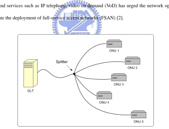
(11) Chapter 1 Introduction Equation Section 1. While the backbone network bandwidth grows tremendously, the access network still remains the bottleneck. Ethernet passive optical networks (EPONs), which represent the convergence of low-cost Ethernet equipment and low-cost fiber infrastructure, appear to be one of the best candidates for the next-generation access network [1]. The low-cost of fiber infrastructure and the high-speed Gigabit Ethernet equipment make EPON very attractive. In addition, the growing demand of broadband services such as IP telephony, video on demand (VoD) has urged the network operator to accelerate the deployment of full-service access networks (FSAN) [2].. Figure 1.1: An EPON network Figure 1.1 shows a tree-topology EPON network. The main components in EPON are optical line terminal (OLT) and optical network unit (ONU). The OLT resides in the central office (CO) and connects the optical access network to the metropolitan area network (MAN) or wide-area network 1.

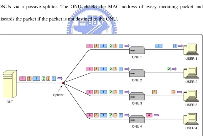
(12) (WAN). The ONU is usually located at either the curb or the end-user location, and provides broadband video, data, and voice services. Passive optical network is a point-to-multipoint optical network with no active elements in the signals’ path from source to destination. The only interior elements used in a PON are passive optical components, such as optical fiber and splitters. An EPON is a PON that carries all data encapsulated in Ethernet frames and is backward compatible with existing IEEE 802.3 Ethernet standards. Moreover, Ethernet is an inexpensive technology that is ubiquitous with a variety of legacy equipment. Due to the growing demand of broadband services such as IP telephony, video on demand (VoD), an EPON with high bandwidth is a promising infrastructure in access network. In the downstream direction, as shown in Figure 1.2, the OLT broadcasts Ethernet packets to all ONUs via a passive splitter. The ONU checks the MAC address of every incoming packet and discards the packet if the packet is not destined to the ONU.. Figure 1.2: Downstream transmissions in EPON. 2.

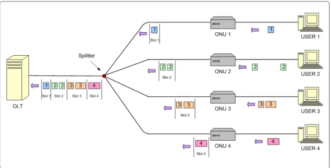
(13) Figure 1.3: Upstream transmissions in EPON In the upstream direction (Figure 1.3), a multiple access scheme should be adopted by the EPON to prevent the collision of packets originating from different ONUs. In wavelength division multiple access (WDMA) scheme [1], each ONU transmits data at different wavelengths. So it would require a tunable receiver at the OLT to receive multiple channels. The drawback of the WDMA scheme is that the WDM components are very expensive. So it is not a good cost-effect scheme in EPON environment. Contention-based multiple access scheme (similar to CSMA/CD) is difficult to implement, because of the directional property of the splitter and the problem to detect collisions in ONUs. The optical code division multiple access (OCDMA) scheme is an alternative solution of supporting multiple access in EPON [3]. It allows active users share the same wavelength band and transmit data simultaneously. OCDMA has several advantages, such as flexibility in network design and security communication capability. But due to no negative power for optical signals, it is more complicated to implement than the other schemes. Compare with the other schemes, TDMA schemes is the most cost-effective solution for EPON network, because it requires only one transceiver in the OLT and it is easy to implement. By adopting TDMA scheme, all ONUs must be synchronized to a common clock. The OLT. 3.

(14) allocates timeslots to ONUs. Each timeslot is able to carry several Ethernet packets. An ONU should buffer packets received from a subscriber and forward the packets to the OLT until its timeslot arrives. If the buffered frames are not able to fill the entire timeslot, idles frames are transmitted. In the OLT, a bandwidth allocation scheme should be provided to allocate timeslots to ONUs in a static or dynamic way. There are many bandwidth allocation schemes proposed for EPON. In [4], a scheduling scheme of fixed timeslot assignment algorithm for EPON was presented. This method adopted a TDMA approach to deliver Ethernet packets. A fixed duration of the timeslot is allocated to each ONU. The advantages of this scheme are easy to implement and able to provide the service for multiple users in a single wavelength. However, the result also showed that a considerable amount of bandwidth was wasted because the unused bandwidth can not be shared to high-loading ONUs (no statistical multiplexing). To increase the channel utilization, an OLT-based polling scheme was proposed in [5], called Interleaved Polling with Adaptive Cycle Time (IPACT). It adopted a polling-based scheme to deliver Ethernet packets from ONUs to OLT over the EPON access network. In IPACT, the duration of the timeslot is variable and the channel utilization is improved. Different scheduling algorithms were studied in [5], i.e. fixed, limited, gated, constant credit, linear credit, and elastic. The limited scheduling algorithm, in which the OLT grants an ONU the requested number of bytes with an upper bound, exhibits the best performance among these algorithms. EPON is expected to support emerging IP-based multimedia traffic with diverse quality-of-service (QoS) requirements [6]. [7] proposed a limited service scheme to support QoS in EPON network. The proposed scheme adopts a gated transmission mechanism (MPCP, Multi-Point Control Protocol) with priority scheduling. A strict-priority (exhaustive) buffer management is adopted and thus, the packet delay of the real-time services is guaranteed. In the proposed scheme, there exists the effect of light-load penalty, where the queueing delay for some traffic classes. 4.

(15) increases when the network load decreases. The authors proposed to adopt a two-stage buffering method or a CBR credit method to eliminate the effect. The two-stage buffering method eliminates the effect but it also increases the delays for higher priority classes. The CBR credit method can only partially eliminates the effect but it requires external knowledge of the arrival process. A promising approach to support differentiated QoS is to employ a central controller that can dynamically allocate bandwidth to end users according to the required bandwidth. Thus, bandwidth management for fair bandwidth allocation among different ONUs will be an important issue for the MAC protocols in the emerging EPON based networks. In [8], [9], and [10], different dynamic bandwidth allocation (DBA) algorithms are proposed. In [8], the authors proposed a DBA algorithm for multimedia services over EPON. They use strict priority queueing and presented control message formats to implement. In [9], the authors proposed a new bandwidth guaranteed polling (BGP) scheme that allows the upstream bandwidth to be shared based on the service level agreement between each subscriber and the operator. In [10], the authors proposed a DBA algorithm with QoS support over EPON-based access network. The DBA algorithms described above can support the guaranteed requirement, i.e. assigned bandwidth, packet delay, and etc., of highest priority service. However, there is no mechanism to take care of non-real-time service, which usually has no delay criterion during packet transmission. So, if the loading is unbalanced but still under the requested bandwidth, the non-real-time data service may experience much of difference in packet delay and packet blocking probability between each ONU. In other words, one of the important issues we want to consider about the non-real-time service is the fairness in average packet delay and average packet blocking probability among all ONUs. In [11] and [12], we find that Queue Length Proportional (QLP) scheme and Longest Queue First (LQF) scheme can achieve the fairness in packet delay and blocking probability, respectively. Based on the idea of QLP and LQF, we proposed a Hybrid LQF-QLP scheduling algorithm and a Hybrid EQL-QLP scheduling algorithm to simultaneously ensure the fairness of packet delay and. 5.

(16) blocking probability. Details of these two proposed schemes are described in Chapter 2. In Chapter 2, we obtain the relationship between the maximum cycle time and the delay criterion of the voice service. That is, the maximum cycle time should be lower than an upper bound in order to meet the QoS requirement of the voice service. This phenomenon is the same as the effect of two-stage buffering which mentioned in [7]. However, shorter maximum cycle time gives rise to the lower channel utilization, because of the irremovable overhead introduced by control messages and guard time. Thus, to improve the channel utilization, we proposed a prediction-based scheduler architecture, which can effectively extend the maximum cycle time. We denote the new scheduling algorithms used in this environment as prediction-based scheduling schemes, i.e. PEQL-PQLP, and PLQF-PQLP. We will discuss the detail in Chapter 3. And finally, a concluding remark is given in Chapter 4.. 6.

(17) Chapter 2 Uplink Scheduling in EPON Access Network Equation Section 2. 2.1 Introduction Rapid deployment of broadband services in the residential and small business area has played an important role in the evolution of access networks. Currently, Ethernet passive optical networks (EPON) [1] are being considered as a promising solution for the next generation access network, due to the convergence of low-cost Ethernet equipment and low-cost of fiber infrastructure. In the upstream direction in EPON, a multiple access scheme should be adopted by the EPON to prevent the collision of packets originating from different ONUs. In the upstream direction of EPON, a multiple access scheme is needed to prevent the collision of packets originating from different ONUs. In [5], a polling-based scheme, called Interleaved Polling with Adaptive Cycle Time (IPACT) was proposed, in which the next ONU is polled before receiving the data form previous ONU. As a result, the channel utilization is higher, compare with traditional TDMA scheme [4], which assign fixed timeslot to all ONUs. Different scheduling algorithms were studied in [5], i.e. fixed, limited, gated, constant credit, linear credit, and elastic. The limited scheduling algorithm, in which the OLT grants an ONU the requested number of bytes with an upper bound, exhibits the best performance among these algorithms. In [7], the author adopted a limited service scheme to support QoS in EPON network. A strict-priority (exhaustive) buffer management is adopted and, thus, the packet delay of the real-time. 7.

(18) services is guaranteed. In the proposed scheme, there exists the effect of light-load penalty, where the queueing delay for some traffic classes increases when the network load decreases. The authors proposed to adopt a two-stage buffering method or a CBR credit method to eliminate the effect. The two-stage buffering method eliminates the effect but it also increases the delays for higher priority classes. The CBR credit method can only partially eliminates the effect but it requires external knowledge of the arrival process. The limited service scheme combined with strict-priority buffer management is a simple way to support different class of service. The QoS of the highest-priority service can be guaranteed. However, the channel utilization is limited if only some ONUs are under high-loading condition, but the others are not. The reason is that the high-loading ONUs can’t be granted to transmit packets which data volume exceeds an upper bound. Moreover, there is no mechanism to take care of non-real-time service, which usually has no delay criterion during packet transmission. So, if the loading is unbalanced but still under the requested bandwidth, the non-real-time service may experience much of difference in packet delay and packet blocking probability between each ONU. One of the important issues we want to consider about the non-real-time service is the fairness in average packet delay and average packet blocking probability among all ONUs. In [11] and [12], we find that Queue Length Proportional (QLP) scheme and Longest Queue First (LQF) scheme can achieve the fairness in packet delay and blocking probability, respectively. Based on the idea of QLP and LQF, we proposed a Hybrid LQF-QLP scheduling algorithm and a Hybrid EQL-QLP scheduling algorithm to simultaneously ensure the fairness of packet delay and blocking probability. The chapter is outlined as follows. In Session 2.2, we introduce the key properties of EPON that would be used in our model. In Session 2.3, we will describe the detailed system model including the EPON system architecture and the scheduler functional block. In Session 2.4, two proposed scheduling algorithms are described. And finally, in Session 2.5, we show the simulation result and make a conclusion.. 8.

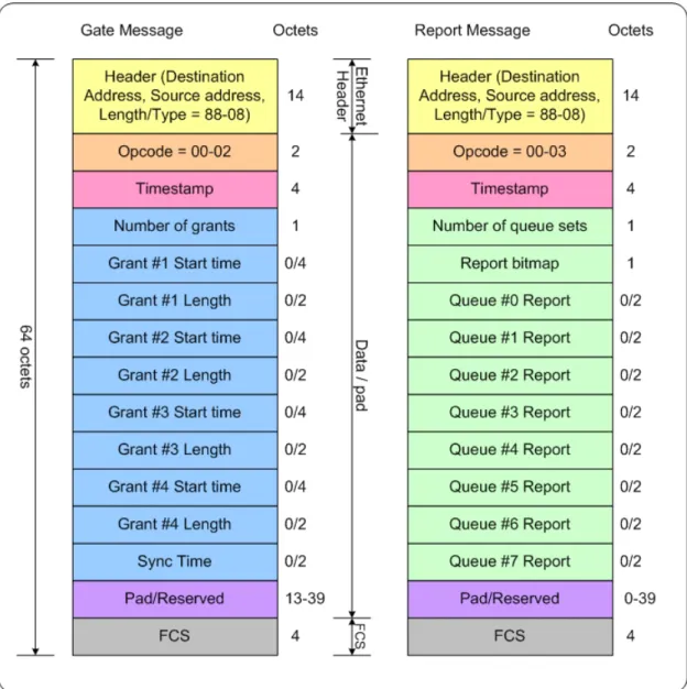
(19) 2.2 Background of EPON The most important packets in EPON network are control packets (Control messages), they are specified in IEEE standard 802.3ah [16]. The work on EPON architecture in the IEEE 802.3ah task force is still in progress. The Multi-Point Control Protocol (MPCP) is chosen by this task force to facilitate the implementation of various bandwidth-allocation algorithms in EPONs. The bandwidth-allocation algorithm is performed based on two types of Ethernet packets, GATE and REPORT, defined by MPCP. A GATE message is sent from the OLT to an ONU, and it used to assign a transmission timeslot. A REPORT message is used by an ONU to convey its local conditions to the OLT to help the OLT make intelligent allocation decisions. These control messages are basic IEEE 802.3 frames, and the packet size of the control messages are all 64-bytes, which is the smallest packet size of IEEE 802.3 frame. The frame structures are shown in Figure 2.1.. 9.

(20) Figure 2.1: GATE message and REPORT message frame format The definitions of each field list as follows:. (a) Header: The header field includes the information about Destination Address, Source Address, and Type. These are basic Ethernet packet field. (b) Opcode: This field identifies the specific control message being encapsulated. The value of GATE message is 2, and the value of REPORT message is 3. (c) Timestamp: The timestamp field conveys the content of the local time register at the time of transmission of the control message. (d) Pad/Reserved: This field is used for the payload of control message. 10.

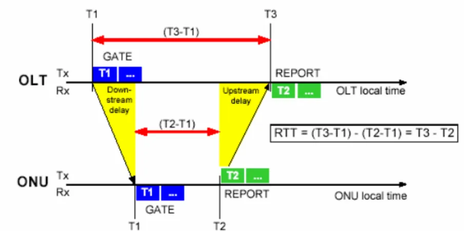
(21) (e) Number of grants/Grant #n start time/Grant #n length: In GATE message, we can have at most 4 grants. Upon the number of grants, we must decide the start time and length of each grant. (f) Number of queue sets/REPORT bitmap/Queue #n report: Similar to GATE message, in REPORT message, at most 8 queues can request the bandwidth based on design purpose. The Timestamp information in an ONU’s REPORT message will be taken into account to get new round-trip-time (RTT) between this ONU and OLT. The measurement of RTT to the source ONU is shown in Figure 2.2.. Figure 2.2: Round-trip time measurement. 11.

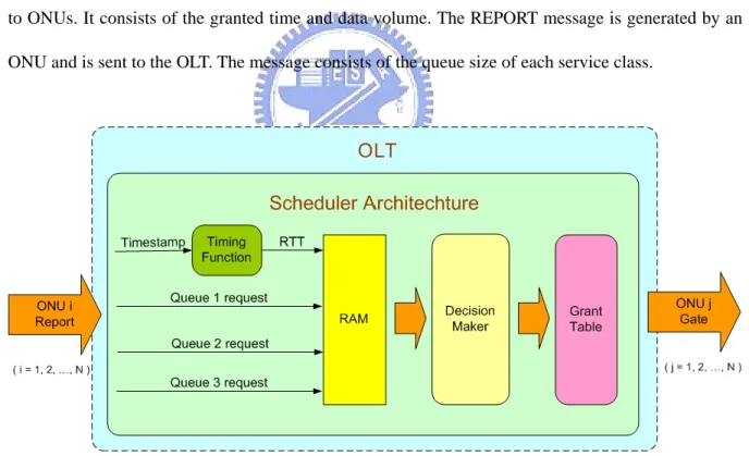
(22) 2.3 System Model 2.3.1 System Architecture We consider an EPON access network consisting of an OLT and N ONUs as shown in Figure 2.3. In the OLT, there is a scheduler, which is responsible for determining the time and data volume that each ONU can transmit during a cycle, where the cycle is the duration between successive scheduling times.. Figure 2.3: The EPON system architecture In each ONU, three independent priority queues are adopted to support real-time voice, real-time video and non-real-time data service. Each class of service is assigned a specific priority, denoted as P1 , P2 , and P3 , respectively, where P1 is the highest priority and P3 is the lowest priority. Incoming packets are classified by traffic classifier and stored in the corresponding priority queue. The queue manager is responsible for receiving GATE message, transmitting appropriate 12.

(23) amount of packets from each queue to OLT, and generating REPORT message when the transmission of user information is finished. The link rate from user equipment to an ONU is RU Mbit/s. The link rate between an ONU and the OLT in upstream and downstream directions are the same and is assumed to be RN Mbit/s. The distance between the OLT and ONUs are different and it results in different round trip time (RTT) for each ONU. We denote L as the maximum distance in kilometer (km) between OLT and an ONU. Even in the same ONU, there still exists some small deviation of RTT compared with previously measured RTT. The RTT updating method can be referred to IEEE 802.3ah standard [16]. The interaction between OLT and ONUs is performed by two major control messages, i.e. GATE message and REPORT message. The GATE message is generated by OLT and is broadcasted to ONUs. It consists of the granted time and data volume. The REPORT message is generated by an ONU and is sent to the OLT. The message consists of the queue size of each service class.. Figure 2.4: Functional modules of a scheduler Now, we focus on the detailed operations of scheduler in OLT. Figure 2.4 depicts the functional modules of a scheduler. The functional modules include a Timing Function, a RAM, a Decision Maker, and a Grant Table. The Timing Function is used to calculate the round-trip-time of each ONU.. 13.

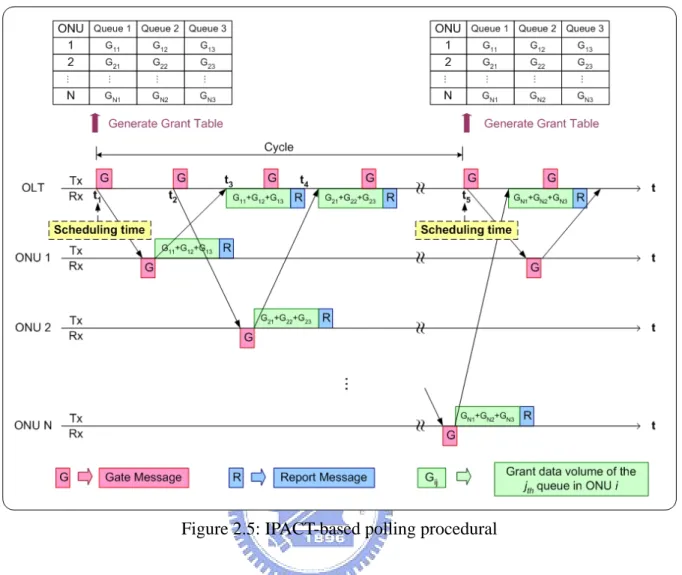
(24) The RAM stores the information of the latest RTT and the amount of requested resource for each ONU. And the Decision Maker is responsible for determining the grant time and data volume of each class of service in every ONU. The proposed scheduling algorithm is implemented in it and we will discuss the detail scheduling operation in later session. And the last functional module in our scheduler is the Grant Table. It is a list that stores the sequence of transmission of all ONUs. It also depicts the granted data volume that each queue in every ONU can transmit during next cycle. The input of scheduler is the REOPORT message, which is defined by MPCP, originated by each ONU. The REPORT message conveys the timestamp information and request data volume of each class of service of an ONU. When the OLT receives a REPORT message originated from ONU. i , the timestamp information will pass to the Timing Function to calculate the latest RTT. Then, the latest RTT and the requested data volume of each class of service obtained from REPORT message will be stored in RAM. During a cycle, the scheduler continues receiving REPORT message from each ONU and storing the information in RAM. Before the end of a cycle, the Decision Maker will start up a scheduling operation. It will take all the information stored in RAM into account. By adopting different scheduling schemes, the amount of grand data volume of each queue in every ONU will be different. Finally, after scheduling, the Grant Table can be generated and OLT can send GATE message to each ONU based on the list of Grant Table. The interaction between OLT and ONUs is based on IPACT, where the duration of the cycle is dynamically changed based on the requested data volumes reported by ONUs. By adopting IPACT-based polling scheme, there is no need to synchronize the ONUs to a common reference clock. Every ONU executes the same procedure driven by the GATE message received from the OLT. Figure 2.5 shows the IPACT-based polling procedural.. 14.

(25) Figure 2.5: IPACT-based polling procedural In Figure 2.5, The Grant Table is generated at scheduling time t1 , in which the granted data volume of each queue, denoted as Gij , i = 1,..., N , j = 1, 2,3, , is determined based on the proposed scheduling algorithm. At time t1 , the OLT sends a GATE message to ONU 1, allowing each queue in ONU 1 to send data volume G11 , G12 , and G13 . When ONU 1 finishes the user data transmission, it would generate REPORT message to inform OLT how much data volume remains in each queue. Before receiving the user data and REOPORT message form ONU 1, OLT sends GATE message to ONU 2 at time t2 , which can be derived by the following equation.. t2 = t4 + g − RTT2 − G / RN = ⎡⎣t3 + ( G11 + G12 + G13 + R ) / RN ⎤⎦ + g − RTT2 − G / RN. (2.1). = ⎡⎣( t1 + RTT1 + G / RN ) + ( G11 + G12 + G13 + R ) / RN ⎤⎦ + g − RTT2 − G / RN ,. where g is the guard interval between the transmission of different ONU, RTTi is the 15.

(26) round trip time of ONU i, G, and R are the GATE message and REPORT message, and. RN is the line rate of EPON. Based on equation (2.1), the times that OLT needs to send GATE message for the other ONUs can be derived. When OLT receives the REPORT message, for example at time t4 , the requested data volume conveyed by the REPORT message will be stored in RAM until next scheduling time t5 . Intuitively, the uplink channel of OLT is almost fully utilized, besides the overhead introduced by REPORT messages and guard times. In other words, the ONUs, which have no data to transmit will not be allocated resource. That leads to a shortened cycle time and results in more frequent polling of active ONUs. Additionally, it is intuitively that the entire scheduling algorithm is located in the OLT. The ONUs do not need to negotiate or acknowledge new parameters, nor do they need to switch to new settings synchronously. Note that the polling procedural is a little difference compared with traditional one. First, OLT can determine the granted data volume of each class of service in an ONU, and ONU also can request the resource of each service class. Second, the requested data volumes conveyed by REPORT messages would be stored in RAM until the scheduling time. After scheduling, the granted data volume that each queue in every ONU can transmit is determined. Third, the data volume that each queue can transmit in an ONU only depended on the corresponding granted data volume conveyed by GATE message.. 16.

(27) 2.4 Scheduling Algorithm The proposed scheduling algorithm is a gated-based scheme, where the scheduler only use the information obtained before the scheduling time. The goal of the scheduling algorithms is to meet the delay bound of voice service, d , and to simultaneously maintain the fairness of both packet delay and packet blocking probability for non-real-time data service. The delay bound of voice service and the overall fairness index, F , for non-real-time data service are defined as follows:. d < d max ,. (2.2). F = x ⋅ I D + (1 − x) ⋅ I B ,. (2.3). where d is the average packet delay of voice service, d max is the delay criterion of voice service, x is a weighting factor ranged form 0 to 1, and I D and I B are the fairness index for average packet delay and average packet blocking probability, respectively. The I D and I B are defined below [20]. ID =. ⎡N ⎤ ⎢ ∑ Di ⎥ ⎣ i =1 ⎦. 2. N. N × ∑ ( Di ). ,. (2.4). ,. (2.5). 2. i =1. IB =. ⎡N ⎤ ⎢ ∑ PB ,i ⎥ ⎣ i =1 ⎦ N. 2. N × ∑ ( PB ,i ). 2. i =1. where Di and PB ,i are the average packet delay and the average packet blocking probability of ONU i, respectively. The overall fairness index F described in equation (2.3) must be as close to 1 as possible. Parameters used in the proposed scheduling algorithm are listed below:. 17.

(28) Qij : requested data volume (in bytes) of the jth service class obtained from REPORT message sent by ONU i. Gij : granted data volume (in bytes) of the jth service class of ONU i encapsulated in GATE message sent by OLT. Qth : the queue length threshold for data (class 3) service. Lmax : the maximum data volume (in bytes) of real-time services each ONU can transmit during one cycle. Tcycle : the cycle time (in sec). Tmax : the maximum cycle time (in sec). b: the guard time (in sec). R: the residual available cabacity (in bytes) after allocating resource to real-time services.. Table 2.1: Parameter descriptions used in scheduling algorithm Assume that at scheduling time, the RAM has stored the requested data volume of each service in every ONU, denoted as Qij , where i = 1,..., N , and j = 1, 2,3 . Then the granted data volume of each class of service, denoted as Gij , where i = 1,..., N , and j = 1, 2,3, is obtained by adopting proposed scheduling algorithm. In the proposed scheduling algorithm, the real-time services are allocated resource first based on the consideration of delay criterion. After that, the resource is fairly allocated to the non-real-time service in each ONU. For real-time services, the granted data volumes, i.e. Gi1 and Gi 2 , are obtained by. ⎧Gi1 = min( Lmax , Qi1 ), ⎨ ⎩Gi 2 = min( Lmax − Gi1 , Qi 2 ),. (2.6). where i = 1, 2,..., N . For voice services, the granted data volumes equal to the requested data volume, but does not exceed Lmax . Similarly, the granted data volumes for video service equal to the requested data volume, but does not exceed Lmax − Gi1. In other words, the granted data volumes of real-time services for each ONU are bounded by Lmax . And, the voice service has the highest priority to share the resource of Lmax . 18.

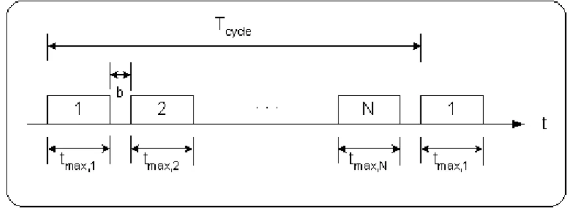
(29) Before describing the scheduling method of data service, we must consider the relationship between the maximum cycle time, denoted as Tmax , and the delay bound of voice service, denoted as. d max . The decision of Tmax must base on the criterion of packet delay requirement of voice service. Let us consider the special case, that is, the load of voice service is extremely high in every ONU and the uplink channel is filled with voice packets. Because all the packets are belong to voice service, the maximum data volume each ONU can transmit must be the same during a cycle. In other words, the duration that each ONU can transmits packets, denoted as tmax,i , i = 1, 2,..., N , is also the same, as shown in Figure 2.6.. Figure 2.6: The case that channel is fully filled with real-time voice packets Then, we can write tmax,1 = tmax,2 = ... = tmax, N =. Lmax , where RN is the uplink transmission RN. rate. In this case, Tcycle is equal to Tmax , which can be derived by. ⎛ ⎛ L ⎞ L ⎞ Tmax = ∑ ( b + tmax,i ) = ∑ ⎜ b + max ⎟ = N ⎜ b + max ⎟ , RN ⎠ RN ⎠ i =1 i =1 ⎝ ⎝ N. N. (2.7). where b is the guard interval. Additionally, the average packet delay of voice packets can be derived. Figure 2.7 shows the arrival and departure of new-coming packets in ONU i .. 19.

(30) Figure 2.7: The average packet delay of voice service The ONU i must report the amount of data volume that accumulates during the first cycle to the OLT at the end of transmission in second cycle. Then, the OLT sends a GATE message, which indicates that the requested data volume could be transmitted in third cycle, to the ONU i. Generally, the requested data volume of voice service reported in second cycle can be completely allowed to transmit in third cycle. Thus, we can derive that the average packet delay of voice service by. d = E[packet delay in 1st Cycle] + E[packet delay in 2nd Cycle] = 0.5 cycle time + 1 cycle time = 1.5 cycle time,. (2.8). where the voice packets arrive at ONU i in first cycle follows uniform distribution. Thus, the packet delay would be 0.5 cycle in first cycle. Moreover, the maximum average packet delay of voice service should be bounded in a delay criterion. Thus, the equation (2.2) can be rewritten by. d ≤ 1.5Tmax ≤ d max .. (2.9). When the granted data volumes of real-time services are determined, the residual available capacity, R, for non-real-time data service can be derived by N. R = (Tmax − N ⋅ b) × RN − ∑ (Gi1 + Gi 2 ).. (2.10). i =1. If the summation of requested data volume of data service is smaller than the residual available. 20.

(31) capacity R , all the requested packets are allowed to transmit in the next cycle, because the resource is adequate to assign to each data service. This situation would happen frequently under light-load condition. But under high-load condition, the resource is usually insufficient. Thus, we need an appropriate scheduling scheme to serve packets well. As mentioned before, for non-real-time data service, the fairness of average packet blocking probability and the fairness of average packet delay among all ONUs are considered. We proposed a Hybrid EQL-QLP scheme and a Hybrid LQF-QLP scheme to achieve this goal. In Session 2.4.1, we introduce the Hybrid LQF-QLP scheme; and in Session 2.4.2, we introduce the Hybrid EQL-QLP scheme.. 2.4.1 Hybrid EQL-QLP scheme The first proposed scheduling scheme for non-real-time data service is Hybrid Equal Queue Length - Queue Length Proportional (Hybrid EQL-QLP) scheme. The inputs are the requested data volumes of data service, Qi 3 , where i = 1,..., N , , and the residual available capacity R . The outputs are the granted data volumes Gi 3 , where i = 1,..., N . . The goal of Hybrid EQL-QLP scheme is to let the fairness index F , defined in equation (2.3), as close to 1 as possible. The granted data volumes of data service are determined by. ⎧ ⎪ ⎪Qi 3 , ⎪ ⎪ Q ⎪ Gi 3 = ⎨ R × N i 3 , ⎪ Q j3 ∑ ⎪ j =1 ⎪ ⎪ f ( R, Q , Q ,...Q ), N3 13 23 ⎪ a ⎩. N. ∑Q j =1. j3. ≤ R,. j3. > R, max{Q13 , Q23 ,...QN 3} ≤ Qth ,. j3. > R, max{Q13 , Q23 ,...QN 3 } > Qth .. N. ∑Q j =1. N. ∑Q j =1. (2.11). where i = 1, 2,..., N . If the summation of the requested data volumes of data service is smaller than the residual available capacity R, all the requested packets are allowed to transmit in the next cycle, 21.

(32) because the resource is adequate to assign to each data service. If the summation of the requested data volume of data service is larger than R, but all of them are smaller than Qth , then the resource assigned to each data service queue is proportional to its requested data volume. However, if the summation of the requested data volumes of data service is larger than R, and one or more than one queue lengths are larger than Qth , then the EQL method is adopted. The method is described as follows. Define an index set K = {k1 , k2 ,...., kn }, where K ∈ {1, 2,...., N } and index k j satisfies. Qk j ,3 > avg , j = 1, 2,..., n. Here, avg meets the equation. ∑ (Q n. j =1. k j ,3. ). − avg = R .. (2.12). The avg can be rewritten as follows. ⎡ n ⎤ ⎢ ∑ Qk j ,3 ⎥ − R j =1 ⎦ avg = ⎣ . n. (2.13). Then the resource assign to each data service queue is. ⎧Q − avg , i ∈ K , Gi 3 = f a ( R, Q13 , Q23 ,..., QN 3 ) = ⎨ i 3 i ∉ K. ⎩0,. (2.14). The resource allocated to each queue, which queue length is larger than avg , is the difference between its queue length and avg . However, there is no resource assigned to the queues, which queue lengths are smaller than avg . The examples of EQL scheme are given in Appendix C.. 2.4.2 Hybrid LQF-QLP scheme The EQL scheme tries to balance the queue sizes of non-real-time data service. It results in a situation that resource has more opportunity to be shared to every queue. If the queue sizes of some data service queue are very large, the LQF scheme is better to alleviate the packet blocking. Thus, we proposed the second scenario for non-real-time data service, named Hybrid Longest Queue First 22.

(33) Queue Length Proportional (Hybrid LQF-QLP) scheme. The idea of this scheme is similar to previous one. Also, the inputs are the requested data volume of data service Qi 3 , i = 1,..., N , and the residual available capacity R, and the outputs are the granted data volume Gi 3 , i = 1,..., N . The resource assignment is written as. ⎧ ⎪ ⎪Qi 3 , ⎪ ⎪ Q ⎪ Gi 3 = ⎨ R × N i 3 , ⎪ Q j3 ∑ ⎪ j =1 ⎪ ⎪ f ( R, Q , Q ,...Q ), N3 13 23 ⎪ b ⎩. N. ∑Q j =1. j3. ≤ R,. j3. > R, max{Q13 , Q23 ,...QN 3 } ≤ Qth ,. j3. > R, max{Q13 , Q23 ,...QN 3 } > Qth .. N. ∑Q j =1. N. ∑Q j =1. (2.15). In equation (2.15), if the summation of queue lengths of data service is smaller than the residual available capacity R, all the requested packets are allowed to transmit in the next cycle, because the resource is adequate to assign to each data service. If the summation of queue lengths of data service is larger than R, but all of them are smaller than Qth , then the resource assign to each data service queue is proportional to its requested data volume. However, if the summation of queue lengths of data service is larger than R, and one or more queue lengths are larger than Qth , then the resource assigned to each data service is described as follows. Define the permutation function π :[1, N ] → [1, N ] , so that Qπ (1),3 ≥ Qπ (2),3 ≥ ... ≥ Qπ ( N ),3 . Note that the permutation function π is the index set with descent order of queue size mapping from the original index.. Gπ ( i ),3 = fb ( R, Q13 ,..., QN 3 ). ⎧min ⎡ max ( Qπ (i ),3 − Qth , 0 ) , R ⎤ + R′ ⋅ Pπ (i ) , i =1, ⎣ ⎦ ⎪⎪ =⎨ i −1 ⎡ ⎤ ⎪min ⎢ max ( Qπ (i ),3 − Qth , 0 ) , R − ∑ Gπ ( j ),3 ⎥ + R′ ⋅ Pπ (i ) , i = 2,..., N , j =1 ⎪⎩ ⎣ ⎦ N ⎛ ⎞ ′ R = max ⎜ R − ∑ max ( Q j 3 − Qth , 0 ), 0 ⎟ , j =1 ⎝ ⎠. 23. (2.16). (2.17).

(34) Pπ (i ) =. Qπ ( i ),3 − max ( Qπ (i ),3 − Qth , 0 ) N. ∑ ⎡⎣Qπ j =1. ( j ),3. − max ( Qπ ( j ),3 − Qth , 0 ) ⎤⎦. .. (2.18). In equation (2.16), the resource allocated to each data service queue consists of two parts of resource assignment. In the first part, the scheduler allocates the emergent queues, which queue occupancies are larger than queue length threshold, an amount of the difference between the queue occupancy and the queue length threshold. In addition, the longest queue has the highest priority to share the resource. In second part, the scheduler allocates the remaining resource, denoted as R′, which is the available resource after allocation in the first part, as derived by equation (2.17), to each ONU again. However, different from the first part, the allocation is based on the proportion of remaining queue occupancies. The goal of first part is to avoid packets blocking, because the queue with larger queue occupancy has higher priority to be served. Thus, the first part is benefit to the fairness of packet blocking probability. In addition, the goal of second part is to avoid that all the resource is allocated to the greedy queues. So, the second part is benefit to the fairness of packet delay. As a result, by adopting the Hybrid LQF-QLP scheme, the fairness of packet delay and packet blocking probability can be considered simultaneously. It fits the original goal of scheduling the non-real-time service.. 2.5 Simulation Result 2.5.1 Traffic Source Models We consider three kinds of services, i.e. real-time voice, real-time video and best-effort data. The priorities of these services are specified by P1 , P2 , and P3 , where class P1 service has the highest priority and class P3 service has the lowest priority.. 24.

(35) Class P1 service is used to emulate a T1 connection. The packet generation rate of P1 service is assumed to be the constant bit rate (CBR). The T1 data arriving from the user is packetized in the ONU by placing 24 bytes of data in a packet. By adding the overhead such as Ethernet, UDP (User Data Protocol) and IP (Internet Protocol) headers in a packet, the packet results in a 70-byte frame and would be generated every 125μs. Hence the data rate of class P1 service is 4.48 Mbps. Class P2 service is used to emulate VBR video streams that exhibit properties of self-similarity and long-range-dependence (LRD). The packet size of this class of service is uniformly distribution and ranges from 64 to 1518 bytes. Class P3 service has the lowest priority. It is used for non-real-time data transfer. The network does not guarantee the delivery or the delay of packets for this service. This class of service is also self-similar and LRD traffic with uniformly-distributed packet size ranged from 64 to 1518 bytes. There is an extensive study, such as [17],[18],[19], and etc, showing that most network traffic flows can be characterized by self-similarity and long-range dependence (LRD). The characteristics of self-similar and LRD are described in Appendix A. To generate self-similar traffic, we used the method described in [18], where the resulting traffic is an aggregation of multiple streams. The structure of the synthetic self-similar traffic generator is shown in Figure 2.8. Each source is performed by ON/OFF Parato-distributed model. The design of the number of sources (K) in a traffic generator is based on the experiment result discussed in [5]. It shows that the burstiness of the traffic (Hurst parameter) does not change with K if the total load is fixed.. 25.

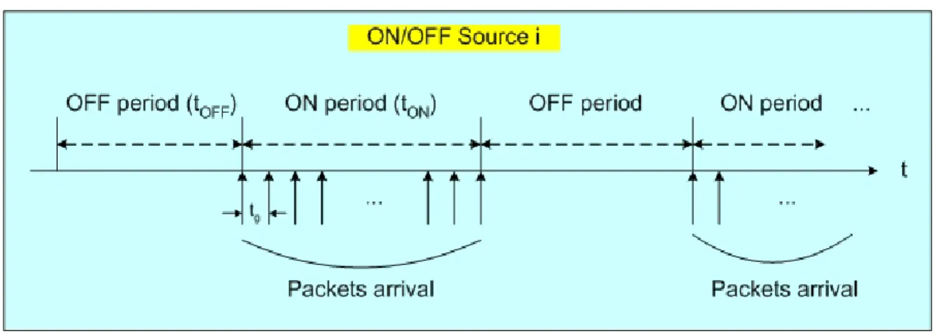
(36) Figure 2.8: Synthetic self-similar traffic generator The traditional ON-OFF source models assume finite variance distributions for the sojourn time in ON and OFF periods. As a result, the aggregation of large number of such sources will not have significant correlation, except possibly in the short range. An extension to such traditional ON-OFF models allows the ON and OFF periods to have infinite variance (high variability or Noah Effect). The superposition of many such sources produces aggregate traffic that exhibits long-range dependence (also called the Joseph Effect) [18].. Figure 2.9: ON/OFF Parato-distributed source i Now we discuss the detail of each source. Figure 2.9 shows the model of source i . The parameters of this model are described as follows:. 26.

(37) The number of packets generated by source i , denoted as Npi , during ON period follows Pareto distribution with a minimum of 1 and maximum of 216-1. Pareto distribution can be defined as follows:. ⎧ α kα f x ( ) , x ≥ k, = ⎪ X α +1 x ⎪ kα ⎪ , α > 1, ⎨µ = − α 1 ⎪ ⎪ 2 k 2α , α > 2, ⎪σ = (α − 2) ⋅ (α − 1) 2 ⎩. (2.19). where α is a shape parameter, and k is a location parameter. We set the shape parameter α = 1.4 . The choice of α was prompted by measurements on actual Ethernet traffic [19]. They reported the measured Hurst parameter of 0.8 for moderate network load. The relationship between the Hurst parameter and the shape parameter α is H = (3 − α ) / 2 [18]. Thus, α = 1.4 should result in. H = 0.8 . During ON period, the packet assumed to immediately follow the previous packet with minimum inter-packet gap t g . We choose t g equals to the standard preamble (8 bytes) of Ethernet packet. Every source has a constant packet size from uniform distribution between 64 and 1518 (in bytes). We denote the packet size generated by source i is Psi . Then, the duration of ON period (tON) of source i can be described as. tON = ( Psi + t g ) × Npi × bytetime ,. (2.20). where bytetime depends on the line rate of EPON, i.e., bytetime = 8 / line rate. OFF periods (intervals between the packet trains) also follow the Parato distribution with the shape parameter α = 1.2 . We used heavier tail for the distribution of the OFF periods represent a stable state in a network, i.e., a network can be in OFF state (no packet transmission) for an unlimitedly long time, while the durations of the ON Periods are ultimately limited by network resources and (necessarily finite) file sizes. To find the minimum value of OFF period (MIN_OFF), 27.

(38) we must consider the average load we want to generate for this self-similar traffic generator. Suppose every source in traffic generator has the same parameters, then the average load, denoted as LOAD, can be represent as. LOAD = K ×. E[ON ] . E[ON ] + E[OFF ]. (2.21). According to equation (2.19), we know that. E[ON] = MIN_ON ×. α = MIN_ON × on_coef, α −1. (2.22). α' = MIN_OFF × off_coef. α '− 1. (2.23). E[OFF] = MIN_OFF ×. By adopting equation (2.21), (2.22) and (2.23), we can derive MIN_OFF as:. MIN_OFF =. on_coef ⎛ K ⎞ × MIN_ON × ⎜ − 1⎟ . off_coef ⎝ LOAD ⎠. (2.24). Then, the minimum value of OFF-period can be decided. By aggregating streams from K independent sources, the realistic self-similar traffic is generated. We use the traffic generator to emulate two kinds of traffic sources, i.e., VBR video streams and best-effort data in our simulation.. 2.5.2 Simulation Environment The system parameters are described as follows:. Parameter. Description. Value. N. Number of ONUs. 16. n. Number of queues in each ONU. 3. Ru. Line rate of user-to-ONU link. 100 Mbps. RN. Line rate between OLT and ONU. 1000 Mbps. Q. The size of each queue. 1 Mbytes. 28.

(39) Maximum data volume of real-time service 5000 bytes. Lmax an ONU can transmit during one cycle tmax b. Maximum slot size of real time traffic Guard time between adjacent slots. 0.04 ms 5 µs. Tmax. Maximum cycle time. 0.72 ms. dmax. The delay bound of voice service. 1.5 ms. x. Waiting factor of overall fairness index. 0.5. Table 2.2: System parameters used in the simulation environment The choice of d max. is based on the specification. International Telecommunication. Standardization Sector (ITU-T) Recommendation G.114 “One-way transmission time” specifies 1.5ms one way propagation delay in access network (digital local exchange). The design of Tmax also based on the delay bound of voice service. To keep the average delay within this bound, we set the parameter tmax = 0.04 ms, results in the maximum cycle time Tmax = 0.72 ms. And now the question is what is the appropriate setting of loads for all ONUs? In general, the loads supported to ONUs are all different. To simplify the simulation, we set the load of a group of ONUs fixed. And the loads of the others are adjusted between different experiments, but remain the same during one experiment. The loads are set as follows:. P0 service: 4.48 Mbps × 16(iid) P1 service: 15 Mbps × 16(iid) P2 service: 15 Mbps × 10(iid) + M × 6(iid), where M = 15 Mbps ~ 80 Mbps Average System Load ≈ 600 Mbps ~ 1000 Mbps The average loads of all P1 services, all P2 services, and ten of P3 services remain a fixed value in every experiment. But the average loads of six of P3 services will change from 15 Mbps to 80 Mbps in different experiment. As a result, the average system load will change approximately from 600 Mbps to 1000 Mbps.. 29.

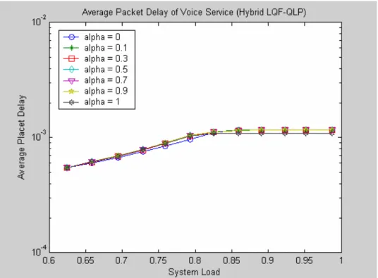
(40) 2.5.3 Simulation Result and Discussion In this session, we show the performance of proposed schemes, i.e. Hybrid EQL-QLP scheme and Hybrid LQF-QLP scheme. Both schemes have queue length thresholds, denoted as Qth , which are the conditions that whether change the mechanism to the other one or not. We define the Qth by. Qth = α × Q,. (2.25). where α is ranged from 0 to 1 and the queue size Q is set to 1 Mbytes. If α equals to 0, then only EQL mechanism is used in Hybrid EQL-QLP scheme; and only LQF mechanism is used in Hybrid LQF-QLP scheme. On the contrary, if α equals to 1, then both schemes only use QLP mechanism. In the following, we first introduce the simulation results of Hybrid LQF-QLP scheme. And then, the performance of Hybrid EQL-QLP scheme is observed. In both schemes, we will check whether the average packet delay of voice service is bounded in delay criterion or not. And we will see the performance of data service. We divide all ONUs into high-loading ONUs and low-loading ONUs. The mean rate of each class of service in low-loading ONUs remains fixed. In high-loading ONUs, the mean rate of real-time services also remains fixed, but the mean rate of best-effort service will change from low to high. We will see the performance of high-loading ONUs and low-loading ONUs individually. After considering the difference between high-loading ONUs and low-loading ONUs, the fairness of best-effort data among all ONUs can be obtained. In Figure 2.10, we show the average packet delay of voice service by adopting Hybrid LQF-QLP scheme. We can see that all the cases, with different value of alpha, have average packet delays of voice service bounded in a value, which is lower than the specified delay criterion (1.5ms). The figure can verify that our system satisfies the basic delay requirement.. 30.

(41) Figure 2.10: Average Packet Delay of Voice Service by adopting Hybrid LQF-QLP Figure 2.11 and Figure 2.12 show the effect of Qth in packet blocking probability by adopting Hybrid LQF-QLP scheme. In Figure 2.11, we can see that LQF mechanism has better performance in average packet blocking probability than QLP mechanism. The reason is that if LQF mechanism is adopted, high-loading ONUs will be assigned the higher priority than low-loading ONUs. So, most of the resource will be assigned to high-loading ONUs, and the packet blocking probability would be lower in high-loading ONUs. Intuitively, the packet blocking probability of low-loading ONUs would be higher by adopting LQF scheme than by adopting QLP scheme. Consequently, the difference of packet blocking probability between high-loading ONUs and low-loading ONUs would be smaller by adopting LQF scheme than by QLP scheme. Finally, we can see the fairness index of packet blocking probability is better in LQF scheme, as shown in Figure 2.12.. 31.

(42) Figure 2.11: Average packet blocking probability (high-loading ONUs) of data service by adopting Hybrid LQF-QLP. Figure 2.12: Packet blocking probability fairness index of data service by adopting Hybrid LQF-QLP When we adjust Qth from 0 to 1, the packet blocking probability would be higher in the. 32.

(43) beginning of the curves, because the characteristic of Hybrid LQF-QLP scheme will approach to the characteristic of QLP mechanism as Qth is close to 1. But if the system load approaches to saturate, the LQF scheme will dominate the performance of packet blocking probability. Because under saturation-load condition, the queue occupancy would increase greatly and almost exceed the condition of Qth more. Thus, there is usually no resource after the first assignment of Hybrid LQF-QLP scheme. As a result, the performance of all cases will approaches to LQF mechanism. And then, in Figure 2.13 and Figure 2.14, we show the effect of Qth in average packet delay and it’s fairness index. By adopting QLP, the resource assign to each ONU is proportional to the requested data volume. So, the variance of average packet delay is lower and the fairness of average packet delay would be higher. If we adopt LQF scheme, the high-loading ONUs get most of the resource. The average packet delay of high-loading ONUs would be decreased. But the average packet delay of low-loading ONUs will increase dramatically, even more than the average packet delay of high-loading ONUs. So the packet delay fairness will be lower than the others.. Figure 2.13: Average Packet Delay (high-loading ONUs) of Data Service by adopting Hybrid LQF-QLP 33.

(44) Figure 2.14: Packet delay fairness index of data service by adopting Hybrid LQF-QLP The result of the overall fairness index F , defined in equation (2.3), is shown in Figure 2.15. We can see that if we consider fairness of packet delay and fairness of packet blocking probability together, the QLP scheme ( Qth = 1 ) and LQF scheme ( Qth = 0 ) would not be the best choices. In this figure, the hybrid scheme with Qth = 0.7 exhibits the best performance.. Figure 2.15: Overall fairness index of data service by adopting Hybrid LQF-QLP 34.

(45) And then, we show the effect of Qth by adopting Hybrid EQL-QLP scheme. Similarly, we must guarantee the average packet delay of voice service. The result of average packet delay for voice service is shown in Figure 2.16. We can see that the average packet delay of voice service still bounds in 1.5ms.. Figure 2.16: Average packet delay of voice service by adopting Hybrid EQL-QLP In Figure 2.17 and Figure 2.18, we show the effect of Qth in average packet blocking probability and fairness of packet blocking probability. The packet blocking probability of high-loading ONUs is higher in QLP than in EQL. It is also because that the most of the resource is assign to high-loading ONUs by adopting EQL scheme. The effect of Qth in packet blocking probability is not obvious when the system load is increasing. Because when a system begins to block packets, the queue occupancies increase dramatically with system load. Under this condition, the EQL scheme will always be adopted. In addition, by adopting Hybrid EQL-QLP scheme, the assignment is independent of Qth when any requested data volume exceeds Qth . Thus, there is no obvious effect in packet blocking probability and fairness of packet blocking probability if we adjust the Qth .. 35.

(46) Figure 2.17: Average packet blocking probability (high-loading ONUs) of data service by adopting Hybrid EQL-QLP. Figure 2.18: Packet blocking probability fairness index of data service by adopting Hybrid EQL-QLP. 36.

(47) We show the result of average packet delay of high-loading ONUs and fairness of average packet delay in Figure 2.19 and Figure 2.20, respectively. Similarly, QLP has better performance in packet delay fairness, because the resource assigned to each user is proportional to the requested data volume. By adopting EQL scheme, the average packet delay of high-loading ONUs is lower, due to fact that most of the resource are assigned to them. But the average packet delay of low-loading ONUs would be increased very much, even exceeds the average packet delay of high-loading ONUs. So the fairness of packet delay would be worse than QLP. Then we focus the effect of Qth in these two figures. For Hybrid EQL-QLP scheme, the design of Qth decides when the algorithm must switch to EQL scheme. If the value of Qth be set lower, then the probability that the algorithm switches from QLP to EQL is higher. It means that we have more opportunity to use EQL schemes. Then the performance will achieve the result of EQL scheme. Finally, we can see the overall fairness index shown in Figure 2.21. The Hybrid EQL-QLP scheme has the best performance when Qth = 0.9 .. Figure 2.19: Average Packet Delay (high-loading ONUs) of Data Service by adopting Hybrid EQL-QLP 37.

(48) Figure 2.20: Packet delay fairness index of data service by adopting Hybrid EQL-QLP. Figure 2.21: Overall fairness index of data service by adopting Hybrid EQL-QLP. 38.

(49) 2.6 Concluding Remarks In this chapter, we proposed two scheduling scheme to obtain the overall fairness which combines the fairness of packet delay and fairness of packet blocking probability. The proposed schemes are Hybrid LQF-QLP and Hybrid EQL-QLP. Each scheme is combined by two basic sub-schemes. We use a queue length threshold to be an adjusting parameter. In the simulation, we define three class of service, i.e. voice, video and data service. The basic requirement of the scheduling algorithm is to meet the delay bound of voice service. Under this condition, we try to improve the fairness of packet delay and fairness packet blocking probability, simultaneously. Simulation results show that by adopting proposed schemes, the overall fairness of data service can be improved compare with traditional scheduling schemes, such as QLP, LQF. It also shows that the Hybrid LQF-QLP scheme has better performance than Hybrid EQL-QLP scheme. We conclude that the proposed scheme can not only maintain the QoS criterion of real-time service, but also support the good fairness for non-real-time service in terms of packet delay and packet blocking probability.. 39.

(50) Chapter 3 Prediction-Based Scheduling Algorithms Equation Section 3. 3.1 Introduction The scheduling architecture proposed in Chapter 2 can guarantee the delay criterion of voice service and support a good fairness to best-effort data service. In order to maintain the delay criterion of voice service, the maximum cycle time should be bounded [7]. We have shown the relationship between average packet delay of voice service and maximum cycle time ( Tmax ) in Chapter 2, where the average packet delay will achieve one and half of the cycle time. In [7], the authors proposed a CBR-credit method to eliminate a phenomenon called light-load penalty. The principle of CBR-credit method is to reserve more resource for CBR traffic. So that the granted transmission data volume of low priority service can be transmit without replacing by CBR traffic. In [10], the authors also use the method similar to CBR-credit to guarantee the packet delay of the highest priority service. The resource reserved for highest priority service is the same as the sum of data volume granted and reported in the last cycle. Thus, the average packet delay of highest priority service can be guaranteed. In [13], the authors proposed a prediction-based LQF scheduling algorithm. They proved that the packet blocking probability is lower than the case which adopts LQF scheduling algorithm only. In IPACT, we know that if the overhead, such as control messages and guard times, remain fixed during every cycle, the throughput will increase with the maximum cycle time ( Tmax ). Thus, we want to increase the cycle time to improve the bandwidth efficiency. To resist the increasing packet delay, we add a predictor in our scheduler architecture. Based on the predicted value of queue occupancy, we can make a better optimization of our system. 40.

(51) In the following of this chapter, we first introduce the system model and the prediction-based scheduler architecture in Session 3.2. And we introduce the principle of the prediction in Session 3.3. Then, the prediction-based scheduling algorithm is expressed in Session 3.4. Finally, the simulation result is obtained in Session 3.5.. 3.2 System Model In the prediction-based system model, the EPON network still remain the same as non-prediction-based EPON network model, besides the scheduler is replaced by prediction-based scheduler, as shown in Figure 3.1. There are also an OLT and N ONUs supported in the prediction-based EPON architecture. And each ONU still can support three classes of services, denoted as P1 , P2 , and P3 , by equipping 3 priority queues. The line rate is RN Mbps between OLT and ONUs and RU Mbps between ONUs and user-site both in the downlink direction and uplink direction. In an ONU, the incoming packets will first be classified into different class of service and then stored in the corresponding priority queue. When ONU receive a GATE message, the queue manager can transmit packets based on the granted transmission data volume. And after transmitting user information, the queue manager will generate the REPORT message to request additional resource.. 41.

(52) Figure 3.1: A prediction-based EPON model The proposed prediction-based scheduler architecture is shown in Figure 3.2. We can see that there exists a predictor in our scheduler architecture. When a REPORT message arrive at OLT, it would be divided into two part of information, i.e. requested data volume of each class of service and the timestamp information of corresponding ONU. The request information will pass into predictor to predict the data volume of new coming packets which received by ONU after generating REPORT message. In other words, the predictor tries to guess the queue occupancies of each queue in corresponding ONU when this ONU receive the GATE message in the next cycle. We will describe the principle of our predictor in the later session. In the meantime, the timestamp information also passes into timing function to calculate the latest round-trip time (RTT). The method of updating the RTT is described in Figure 2.2. After the operation of timing function and predictor, the latest RTT and predicted queue occupancies will be stored in RAM. During a cycle, OLT will receive N REPORT messages from N ONUs, and they all will be stored until next scheduling time.. 42.

(53) Figure 3.2: The prediction-based scheduler architecture Before the beginning of the next cycle, the Decision Maker will calculate the timing and grant how much data volume each queue can transmit in the next cycle. The input is all the information stored in RAM, such as the latest RTT of each ONU and predicted queue occupancy of each queue in each ONU. After scheduling, the Grant Table would be updated. Finally, based on the Grant Table, the OLT can send GATE messages to ONUs so that ONUs know how much data volume each service can transmit. In addition, we also adopt IPACT to be the interaction method between OLT and ONUs. In principle, IPACT uses an interleaved polling approach, where the next ONU is polled before the transmission from the previous one has arrived. The detail of IPACT-based polling procedure is introduced in Figure 2.5.. 3.3 Predictor The concept of prediction is shown in Figure 3.3. We see that before the beginning of Cycle (n+1), we must do a scheduling operation so that the packets transmitted by ONU i (we assume that ONU i is the first candidate to transmit packets in a cycle) can be received in OLT just at the time. 43.

(54) that last candidate finished its transition in Cycle (n).. Figure 3.3: The concept of prediction method Assume that OLT need do a scheduling operation at t0 . During Cycle (n), the OLT has received user data, which data volume is denoted as Di j [n], and REPORT messages, in which the request data volume is denoted as Qi j [n], where i = 1,..., N , and j = 1, 2,3. In addition, we denote. Vi j [n] as the data volume of arrival packets, where i = 1,..., N , and j = 1, 2,3. When OLT receives a REPORT message, in which the request data volume Qi j [n] is included, then the data volume of arrival packets Vi j [n] can be obtained by. Vi j [n] = Dij [n] + Qij [n] − Qij [n − 1] ,. (3.1). where i is ranged from 1 to N, and j is ranged from 1 to 3. Now we define the prediction order K as the number of samples we want to reference in the past history. Then prediction value of. Vi j [n + 1], denoted as Vi′j [n + 1], can be obtained by Vi ′j [n + 1] =. 1 K −1 ∑ Vij [n − m]. k m =0. (3.2). Finally, we define the predicted queue occupancy of class j service in ONU i as Oi j , and it 44.

(55) can be derived by. Oij [n + 1] = Qij [n] + Vij′[n + 1].. (3.3). When OLT receives a REPORT message, it will generate predicted queue occupancy for each class of service and store them in RAM. Then, at scheduling time t0 , the scheduler can use the predicted queue occupancies to fairly assign the resource.. 3.4 Prediction-based Scheduling Algorithm Suppose. that. we. have. a. set. of. predicted. queue. occupancies,. i.e.. Oi j , where i = 1,..., N , and j = 1, 2,3 , at scheduling time, we want to design the granted data volumes, i.e. Gi j , where i = 1,..., N , and j = 1, 2,3 , that each queue can transmit during next cycle. Also, we consider three kinds of service. The real time services, i.e. voice and video service, have higher priority and the non-real-time service, i.e. data service, has lower priority. In our scheduling algorithm, we allocate the resource to real-time services as more as possible, that is. Gi1 = min( Lmax , Oi1 ),. (3.4). Gi 2 = min( Lmax − Gi1 , Oi 2 ).. (3.5). Then we can derive the residual available capacity R as follows: N. R = (Tmax − N ⋅ b) × RN - ∑ (Gi1 + Gi 2 ).. (3.6). i =1. In the following session, we introduce the scheduling mechanisms for non-real-time data service. It is similar to the ones introduced in Chapter 2, besides the input of the scheduler is replaced by predicted queue occupancies. In Session 3.4.1, we explain the operation of Hybrid PEQL-PQLP scheme; and in Session 3.4.2, a detailed description of Hybrid PLQF-PQLP scheme is given.. 45.