適應性累積和損失管制圖之研究 - 政大學術集成

全文

(1)國立政治大學統計學系碩士學位論文指導教授:楊素芬博士適應性累積和損失管制圖之研究政治. 大. 立 The Study of Adaptive CUSUM Loss Control Charts ‧. ‧ 國. 學. n. er. io. sit. y. Nat. al. Ch. engchi. i n U. v. 研究生：林政憲撰中華民國九十九年六月.

(2) 謝辭經過了兩年來的努力學習及多次的校訂，終於完成了此論文。回首這兩年的研究所時光，除了在學術上的增進外，也包含了面對挑戰、解決問題以及對自己負責的學習態度。在這最後收成喜悅的時候，我要感謝許多人對我的鼓勵及幫助。感謝我的指導老師─楊素芬教授。老師不僅對於學術研究十分熱忱與專注，對於學生的指導也是不遺餘力，感謝老師一直以來的叮嚀，無論是在品管知識上或是做人處事上，都給了我很多的建議，讓我有信心可以面對未來的挑戰。感謝我的口試委員曾勝滄教授與呂明哲教授，謝謝兩位老師在口試時給我寶貴的意見，. 政治大感謝我研究所的同學們，在這兩年的學習中，大家互相幫忙、勉勵，讓我留下一個美立. 讓我知道我的論文有哪些地方可以再加強並且深入探討。. 好的記憶。. ‧ 國. 學. 感謝我的夥伴們宜臻、伊萱和亮妤，謝謝妳們這兩年來的照顧，我會永遠記得我們一. ‧. 起學習品管的日子。. io. er. 後，我想將這個喜悅與你們一同分享。. sit. y. Nat. 感謝我的家人，因為有你們的支持與體諒，我才能心無旁騖的完成研究所的學業。最. 本研究承蒙行政院國家科學委員會補助，計畫編號 NSC-96-2118-M-004-001-MY2、. al. n. v i n NSC-98-2118-M-004-005-MY2，及政治大學商學院服務創新頂尖研究中心(CSI)補助，特此 Ch engchi U 感謝。. 林政憲謹致中華民國九十九年六月.

(3) ABSTRACT The CUSUM control charts have been widely used in detecting small process shifts since it was first introduced by Page (1954). And recent studies have shown that adaptive charts can improve the efficiency and performance of traditional Shewhart charts. To monitor the process mean and variance in a single chart, the loss function is used as a measure statistic in this article. The loss function can measure the process quality loss while the process mean and/or variance has shifted. This study combines the three features: adaption, CUSUM and the loss function, and proposes the optimal VSSI, VSI, and FP CUSUM Loss chart. The performance of the proposed. 政治大 to Signal (ANOS). The ATS and ANOS calculations are based on Markov chain approach. The 立. charts is measured by using Average Time to Signal (ATS) and Average Number of Observations. performance comparisons between the proposed charts and some existing charts, such as. ‧ 國. 學. X + S 2 charts and CUSUM X + S 2 charts, are illustrated by numerical analyses and some. ‧. examples. From the results of the numerical analyses, it shows that the optimal VSSI CUSUM. y. Nat. Loss chart has better performance than the optimal VSI CUSUM Loss chart, optimal FP. er. io. sit. CUSUM Loss chart, CUSUM X + S 2 charts and X + S 2 charts. Furthermore, using a single chart to monitor a process is not only easier but more efficient than using two charts. al. n. v i n simultaneously. Hence, the adaptiveC CUSUM Loss charts U h e n g c h i are recommended in real process.. KEYWORDS: CUSUM control chart; Adaptive control chart; VSI control chart; VSS control chart; VSSI control chart; Loss function; Markov chain; Genetic algorithm..

(4) CONTENTS 1. INTRODUCTION .................................................................................................... 1 2. DESCRIPTION OF IN-CONTROL AND OUT-OF-CONTROL PROCESS QUALITY VARIABLES ............................................................................................................... 3 3. OPTIMAL FP CUSUM LOSS CHART ...................................................................... 4 3.1 Description of the optimal FP CUSUM Loss chart ............................................................................ 4 3.2 Design of the optimal FP CUSUM Loss chart ................................................................................... 6 3.2.1 The Performance Measurement ................................................................................................... 6. 政治大. 3.2.2 ARL calculation based on Markov chain approach..................................................................... 6. 立. 3.2.3 Computing the upper control limit H under a specified k ........................................................... 9. ‧ 國. 學. 3.2.4 The procedure of acquiring the optimal reference value k and upper control limit H................. 9 3.3 Numerical analyses for the optimal FP CUSUM Loss chart ............................................................ 10. ‧. 3.4 Example for the optimal FP CUSUM Loss Chart ............................................................................ 16. sit. y. Nat. 4. OPTIMAL VSI CUSUM LOSS CHART .................................................................. 19. al. er. io. 4.1 Description of the optimal VSI CUSUM Loss chart ........................................................................ 19. v. n. 4.2 Design of the optimal VSI CUSUM Loss chart ............................................................................... 21. Ch. engchi. i n U. 4.2.1 The performance measurement ................................................................................................. 21 4.2.2 ATS calculation based on Markov chain approach ................................................................... 22 4.2.3 Computing the warning control limit W under k and H ............................................................ 24 4.2.4 The procedure of acquiring the optimal process parameters ..................................................... 24 4.3 Numerical analyses for the optimal VSI CUSUM Loss chart .......................................................... 25 4.4 Example for the optimal VSI CUSUM Loss Chart .......................................................................... 29. 5. OPTIMAL VSSI CUSUM LOSS CHART ................................................................ 32 5.1 Description of the optimal VSSI CUSUM Loss chart...................................................................... 32 5.2 Design of the optimal VSSI CUSUM Loss chart ............................................................................. 35 I.

(5) 5.2.1 The performance measurement ................................................................................................. 35 5.2.2 ATS and ANOS calculations based on Markov chain approach ............................................... 36 5.2.3 Computing the warning control limit W under k and H ............................................................ 38 5.2.4 Computing the long sampling interval t1 ................................................................................... 38 5.2.5 The procedure of acquiring the optimal process parameters ..................................................... 39 5.3 Numerical analyses for the optimal VSSI CUSUM Loss chart........................................................ 40 5.4 Example for the optimal VSSI CUSUM Loss Chart ........................................................................ 44. 6. CONCLUSION AND FUTURE STUDY .............................................................................. 47 REFERENCES ............................................................................................................................ 48. 政治大 APPENDIX .................................................................................................................................. 51 立 ‧. ‧ 國. 學. n. er. io. sit. y. Nat. al. Ch. engchi. II. i n U. v.

(6) LIST OF TABLES 1. Table 3.1 The optimal (k, H ) values under the specified n0 = 4, δ 3 = 0 and ARL0 = 370 11 2. Table 3.2 The optimal (k, H ) values under the specified n0 = 4, δ 3 = 1 and ARL0 = 370 . 11 3. Table 3.3 The ARL1 values of the optimal FP CUSUM Loss chart under the specified. n0 = 4 and ARL0 = 370 ......................................................................................... 12 4. Table 3.4 The Saved Time between the optimal FP CUSUM Loss chart and X + S 2 charts under specified n0 = 4 and ARL0 = 370 .............................................................. 15. 政治大 5. Table 4.1 The ATSs and Saved times for the optimal VSI, FP CUSUM Loss charts and 立. ‧ 國. 學. X + S 2 charts .......................................................................................................... 27. 6. Table 5.1 The ATSs, ANOSs and Saved times for the optimal VSSI, FP CUSUM Loss charts. ‧. and X + S 2 charts .................................................................................................. 41. n. al. er. io. sit. y. Nat. 7. Table 5.2 Efficiency comparison between five charts under δ1 = 0.5, δ2 = 1.5 ...................... 45. Ch. engchi. III. i n U. v.

(7) LIST OF FIGURES 1. Figure 2.1 The difference between in-control process and out-of-control process ..................... 3 2. Figure 3.1 The structure of the optimal FP CUSUM Loss Chart ................................................ 5 3. Figure 3.2 States of the optimal FP CUSUM Loss chart ............................................................ 7 4. Figure 3.3 Main effects plot for δ 1 , δ 2 , δ 3 on ARL1 of the optimal FP CUSUM Loss chart ... 14 5. Figure 3.4 Main effects plot for Saved Time of δ 1 , δ 2 , δ 3 comparing to X + S 2 charts .......... 16 6. Figure 3.5 Trial optimal CUSUM Loss Chart ........................................................................... 17. 政治大. 7. Figure 3.6 Trial X Chart ........................................................................................................ 17. 立. 8. Figure 3.7 Trial S 2 Chart........................................................................................................ 17. ‧ 國. 學. 9. Figure 3.8 Optimal CUSUM Loss Chart ................................................................................... 18. ‧. 10. Figure 3.9 X Chart ............................................................................................................... 18. sit. y. Nat. 11. Figure 3.10 S 2 Chart............................................................................................................. 18. n. al. er. io. 12. Figure 4.1 The structure of the optimal VSI CUSUM Loss Chart .......................................... 20. i n U. v. 13. Figure 4.2 States of the optimal VSI CUSUM Loss chart ...................................................... 22. Ch. engchi. 14. Figure 4.3 The genetic algorithm procedure of the optimal VSI CUSUM Loss chart ........... 25 15. Figure 4.4 The main effect plot for δ 1 , δ 2 , δ 3 on average ATS1 of the optimal VSI CUSUM Loss chart ............................................................................................................... 28 16. Figure 4.5 The main effect plot for δ 1 , δ 2 , δ 3 on Saved Time* .............................................. 28 17. Figure 4.6 The main effect plot for δ 1 , δ 2 , δ 3 on Saved Time** ........................................... 28 18. Figure 4.7 Trial optimal VSI CUSUM Loss Chart ................................................................. 29 19. Figure 4.8 Trial X Chart ...................................................................................................... 30 20. Figure 4.9 Trial S 2 Chart...................................................................................................... 30 IV.

(8) 21. Figure 4.10 Optimal VSI CUSUM Loss Chart ....................................................................... 31 22. Figure 4.11 X Chart ............................................................................................................. 31 23. Figure 4.12 S 2 Chart............................................................................................................. 31 24. Figure 5.1 The structure of the optimal VSSI CUSUM Loss Chart ....................................... 34 25. Figure 5.2 States of the optimal VSSI CUSUM Loss chart .................................................... 36 26. Figure 5.3 The genetic algorithm procedure of the optimal VSSI CUSUM Loss chart ......... 39 27. Figure 5.4 The main effect plot for δ 1 , δ 2 , δ 3 on average ATS1 of the optimal VSSI CUSUM. 政治大 28. Figure 5.5 The main effect plot for δ , δ , δ on average ANOS of the optimal VSSI 立. Loss chart ............................................................................................................... 42 1. 2. 1. 3. ‧ 國. 學. CUSUM Loss chart ............................................................................................... 42 29. Figure 5.6 The main effect plot for δ 1 , δ 2 , δ 3 on Saved Time* ............................................. 42. ‧. 30. Figure 5.7 The main effect plot for δ 1 , δ 2 , δ 3 on Saved ANOS* ........................................... 43. y. Nat. er. io. sit. 31. Figure 5.8 The main effect plot for δ 1 , δ 2 , δ 3 on Saved Time** ........................................... 43 32. Figure 5.9 The main effect plot for δ 1 , δ 2 , δ 3 on Saved ANOS** ......................................... 43. al. n. v i n C 33. Figure 5.10 Optimal VSSI CUSUMhLoss 45 e nChart hi U g c..................................................................... 34. Figure 5.11 Standardized X Chart with variable sample size.............................................. 45 35. Figure 5.12 S 2 Chart with variable sample size ................................................................... 46. V.

(9) 1. INTRODUCTION Control charts are one of the primary tools in statistical quality control. These charts are useful for monitoring and detecting whether the process is in-control or out-of-control. Since Walter Shewhart first introduced the control chart technique in 1924, control charts have found widespread application in various industrial manufacturing processes. However, the main drawback of Shewhart control charts is it is insensitivity to small shifts in quality characteristics. So CUSUM charts, first proposed by Page (1954), make up for some of the defects of Shewhart charts by providing good detection capability for small process mean shifts. However, it is also importance of monitoring the process variability. Some papers discussed about this topic.. 政治大. Hawkins (1981, 1993a) proposed a CUSUM chart for monitoring scale parameter. Hawkins and. 立. Olwell (1998) proposed a CUSUM variance control chart to monitor process variance. Gan. ‧ 國. 學. (1995) investigated a static scheme consisting of two one-sided CUSUM mean charts and two one-sided CUSUM variance charts for monitoring the process mean and variance. ‧. simultaneously.. y. Nat. sit. From another aspect, the usual practice of using a control chart to monitor a process is to. n. al. er. io. take samples with fixed time intervals or sample sizes. Recent studies show that a control chart. i n U. v. with variable sampling interval (VSI), variable sample size (VSS), or even both features (VSSI). Ch. engchi. allows the sampling time intervals or sample sizes to be changed according to the values of sample readings, which indicate the current process state. Reynolds et al. (1988) and Chengalur et al. (1989) studied the use of VSI X chart to detect process mean shifts. Costa (1999) proposed a VSI X &R chart to monitor both mean and variance shifts. Prabhu et al. (1994) proposed the combined adaptive chart, it’s also VSSI X chart, by combining VSI and VSS features. Reynolds et al. (1990) first used the adaption feature in CUSUM chart and proposed VSI CUSUM chart, and Annadi et al. (1995) developed a VSS CUSUM chart for controlling mean shifts. Arnold and Reynolds (2001) developed the VSSI CUSUM charts for one-sided and two-sided mean shifts. Approaches that use two possible sampling intervals and sample sizes are 1.

(10) easy to implement and are used by most researchers (Reynolds et al., 1988; Daudin, 1992; Wu and Luo, 2004). These studies show that adaptive VSI, VSS and VSSI charts are more efficient than corresponding static charts with fixed sampling intervals and sample sizes. Because the process mean and variability are both important factors in a process, researchers have paid considerable attention to joint charts for monitoring the process mean and variance. Costa and Rahim (2000, 2004) developed economic models for joint X and R charts. Gan (1995) considered joint EWMA charts; Albin et al. (1997) studied an X chart and an EWMA chart for individual observations. However, using two or more charts to monitor a process is. 政治大 shifts and an increasing variance shift would simplify design and operation. Recent studies 立. inconvenient and hard to implement. A single chart capable of monitoring both two-sided mean. propose various kinds of single charts for this purpose, including the MaxMin EWMA chart. ‧ 國. 學. (Amin et al. 1999) and the MaxEWMA chart (Chen et al. 2001). Reynolds and Gosh (1981) and. ‧. Cyrus (1997) developed the L chart. This chart is based on the concept of a loss function, which. sit. y. Nat. can measure the cost of the poor quality. Wu and Tian (2006) extended the loss function to a. io. er. weighted loss function as statistic and proposed the weighted loss function (WL) control charts. After that, Zhang and Wu proposed VSI weighted loss function CUSUM (WLC) chart in 2006,. al. n. v i n C hin 2007. The currentUstudy combines these control chart VSS WLC chart and VSSI WLC chart engchi features, i.e., VSI, VSSI, CUSUM and the loss function, into a proposed optimal FP CUSUM Loss chart, optimal VSI CUSUM Loss chart and optimal VSSI CUSUM Loss chart. The following discussion shows how to construct these proposed charts, and how to determine the optimal process parameters using a genetic algorithm. The numerical analyses in this study. compare the performance of the proposed charts with that of the optimal FP CUSUM Loss chart and traditional X + S 2 charts. Finally, this study also provides examples to show the detection speed of the proposed charts and traditional X + S 2 charts, and revealing the differences between them. 2.

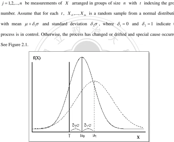
(11) 2. DESCRIPTION OF IN-CONTROL AND OUT-OF-CONTROL PROCESS QUALITY VARIABLES Let X denote a certain quality characteristic of a process, µ denote the process mean,. σ denote the process standard deviation, and T = µ − δ 3σ denote the target value of the process, if δ 3 = 0 that represents the process target equal the process mean. Let X tj , t = 1,2,3,... , j = 1,2,..., n be measurements of X arranged in groups of size n with t indexing the group. number. Assume that for each t , X t1 ,..., X tn is a random sample from a normal distribution with mean µ + δ 1σ and standard deviation δ 2σ , where δ 1 = 0 and δ 2 = 1 indicate the. 政治大. process is in control. Otherwise, the process has changed or drifted and special cause occurred.. 立. See Figure 2.1.. ‧. ‧ 國. 學. n. er. io. sit. y. Nat. al. Ch. engchi. i n U. v. Figure 2.1 The difference between in-control process and out-of-control process. In short, the study has the following assumptions. ( (. ). i.i.d.  2 X ,...,X  t1 tn ~ N μ,σ , if the process is in control  i.i.d.  X t1 ,...,X tn ~ N μ + δ1σ,δ 22 σ 2 ,δ1 ≠ 0 , δ 2 > 1, if the process is out of control. ). 3.

(12) 3. OPTIMAL FP CUSUM LOSS CHART To improve the efficiency and performance of X + S 2 charts in small process shifts, an optimal FP (Fixed Parameters) CUSUM Loss chart is proposed. This chart uses the loss function as a statistic that can monitor the process mean and variance using a single chart. This feature makes it easy to implement and quick to detect the out-of-control process in real manufacturing process. The high-tech process demands the quality strictly. Even though the quality characteristics have very small shifts, it may cause a big loss to the company, so detecting small shifts is more important. The proposed optimal FP CUSUM Loss chart with an optimal reference. 政治大 to design this chart and how to立 find the optimal reference value k by numerical method. A. value k increases the capability of detecting small shifts. The following sections will show how. ‧ 國. 學. numerical example is given to show how to implement the proposed chart and compare the detection speed with Shewhart X + S 2 charts. The numerical analyses show the results include. ‧. (1) The optimal reference value found under different shift scales of process mean and variance.. sit. n. al. er. io. different shift scales.. y. Nat. (2) Choose six combinations of process parameters to compare their detection speeds under. i n U. v. (3) Compare the detection speed between the proposed optimal FP CUSUM Loss chart and. Ch. engchi. Shewhart X + S 2 charts under different shift scales.. 3.1 Description of the optimal FP CUSUM Loss chart The following statistic represents the average quality loss n. L*t =. ∑(X j =1. tj. − T )2. n. , t = 1,2,.... (3.1). To standardize the statistic of the average quality loss, we can transform it into a new statistic Lt as follows Lt =. nL*t. σ2. , t = 1,2,.... (3.2) 4.

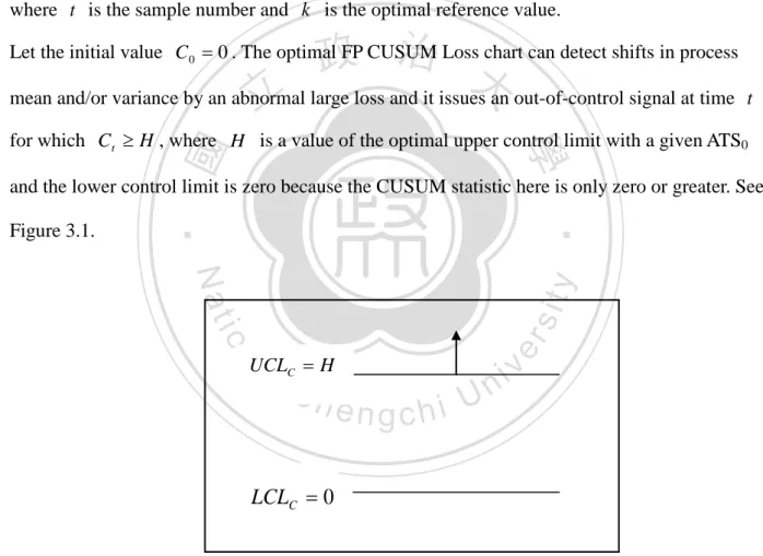
(13) When the process is in control, Lt ~ χ n2,λ0 with the non-central chi square distribution of degrees of freedom n and non-central parameter λ0 = nδ 32 . When the process is out of control, Lt ~ δ 22 χ n2,λ1 with the non-central chi square distribution of degrees of freedom n and non-central parameter λ1 = n((δ 1 + δ 3 ) / δ 2 ) . 2. Define the CUSUM statistic as follows C t = max(0, C t −1 + Lt − k ), t = 1,2,.... (3.3). where t is the sample number and k is the optimal reference value.. 政治大 mean and/or variance by an abnormal 立 large loss and it issues an out-of-control signal at time t. Let the initial value C 0 = 0 . The optimal FP CUSUM Loss chart can detect shifts in process. ‧ 國. 學. for which C t ≥ H , where H is a value of the optimal upper control limit with a given ATS0 and the lower control limit is zero because the CUSUM statistic here is only zero or greater. See. ‧. io. sit. y. Nat. al. er. Figure 3.1.. n. UCLC = H. Ch. engchi. i n U. v. LCLC = 0. Figure 3.1 The structure of the optimal FP CUSUM Loss Chart. 5.

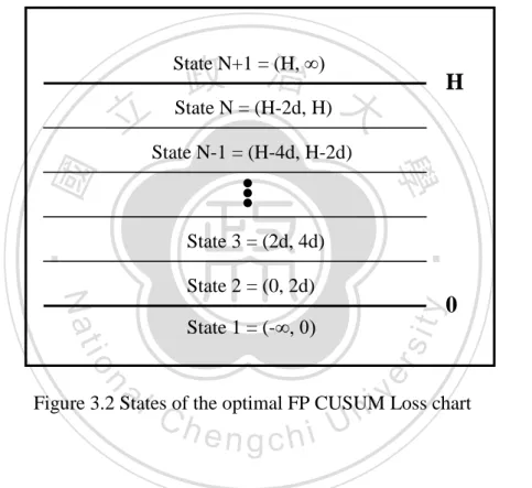
(14) 3.2 Design of the optimal FP CUSUM Loss chart 3.2.1 The Performance Measurement The average run length (ARL) of a chart represents the performance of a CUSUM chart. Ideally, a CUSUM chart should have a large ARL when the process is in control and a small ARL when the process is out of control. Define ARL0 as the average run length to signal when the process is in control, and ARL1 as the average run length to signal when the process is out of control. To compare the performance between the proposed optimal FP CUSUM Loss chart and. 政治ARL 大− ARL ARL. X + S 2 charts, here define an index : Saved Time =. 立. X +S 2. X +S. FP. × 100% , where ARLX + S 2. 2. ‧ 國. 學. denote as an ARL1 of X + S 2 charts and ARLFP denote as an ARL1 of the optimal FP CUSUM Loss chart. The value of the Saved Time shows that the proposed optimal FP CUSUM Loss chart. ‧. saves how much proportion of time in detecting process shifts comparing to X + S 2 charts while. y. Nat. n. al. er. io. sit. the process is out of control.. i n U. 3.2.2 ARL calculation based on Markov chain approach. Ch. engchi. v. Brook and Evans (1972) developed an ARL calculation method based on Markov chain theory. The Markov chain approach is applied to calculate the ARL of the proposed FP CUSUM Loss chart for different combinations of δ1 , δ 2 and δ 3 . The following method shows the ARL calculation in detail. Divide the interval (0, H ) into N-1 subintervals with equal width 2d, where d =. H . 2( N − 1). Then let the interval (−∞,0] as the 1st subinterval and its midpoint m1 = 0 ; the interval (mi − d , mi + d ), i = 2,3,..., N as the i th subinterval, where mi =. (2i − 3) H . See Figure 3.2. 2( N − 1). Define the i th subinterval as the i th state. A state is said to be a transient state, if it can 6.

(15) transfer to another states. A state is said to be an absorbing state, if it cannot transfer to another states. The state 1 to N are all transient states, because when a sample point falls within these states, it indicates the process is in control, and the process keeps going. The action region above the control limit is defined as the N + 1th state that represents the absorbing state, because when a sample point falls in the state, an out-of-control signal is given, and the process is stopped. Thus, the ARL is the expected run length to absorption.. 政治大 State N = (H-2d, H). State N+1 = (H, ∞). 立. H. 學. ●●●. ‧ 國. State N-1 = (H-4d, H-2d). ‧. State 3 = (2d, 4d). 0. y. Nat. State 2 = (0, 2d). n. er. io. al. sit. State 1 = (-∞, 0). i n U. v. Figure 3.2 States of the optimal FP CUSUM Loss chart. Ch. engchi. The transition probability Pij is the probability of statistic C t −1 in state i at time t − 1 moving to state j at time t. That is the probability that C t lays in state j, conditioned on C t −1 being equal to the midpoint of the i th subinterval. Pi1 = P(C t ≤ 0 | C t −1 = mi ). = P(C t −1 + Lt − k ≤ 0 | C t −1 = mi ) = P(Lt ≤ −mi + k ). = Fχ 2. n ,λ. ((− m. i. (3.4). ). + k ) / δ 22 , i = 1,2,..., N , t = 1,2,3,.... 7.

(16) Pij = P (m j − d ≤ C t < m j + d | C t −1 = mi ). = P (m j − d ≤ C t −1 + Lt − k < m j + d | C t −1 = mi ) = P (m j − mi − d + k ≤ Lt < m j − mi + d + k ). = Fχ 2. n ,λ. ((m. j. ). − mi + d + k ) / δ 22 − Fχ 2. n ,λ. ((m. j. ). − mi − d + k ) / δ 22 , i = 1,2,..., N , j ≠ 1, t = 1,2,3,.... (3.5) where Fχ 2 (•) denote the cumulative non-central chi-square distribution with degrees of n ,λ. freedom n and non-central parameter λ . Define P as a ( N + 1) × ( N + 1) transition probability matrix. Q be the matrix obtained from P by deleting row N+1 and column N+1. In other words, Q = Pij , i, j = 1,..., N is the. 政治大 transition probability matrix among the in-control states. 立. Refer to Brook and Evan (1972), the following results are applied. Let Ri be the run. ‧ 國. 學. length taken starting from state i to reach the absorbing state for the first time, and let FR (r ) be. ‧. a vector of length N whose elements are the cumulative distributions of run length starting from. y. Nat. states 1, 2,…, N, that is. ). al. n. (. FR (r ) = I − Q r ⋅ 1. T. (3.6). er. io Then by matrix form. sit. FR (r ) = (P(R1 ≤ r ), P(R2 ≤ r ),..., P(R N ≤ r )) , r = 1,2,.... Ch. engchi. i n U. v. (3.7). And the first element of FR (r ) gives the cumulative probability for run length for a CUSUM scheme starting from state 1 (or C 0 = 0 ). Let L R (r ) be a vector of length N whose elements are the values of the probability functions of run length starting from state 1, 2,…, N, that is. L R (r ) = (P(R1 = r ), P(R2 = r ),..., P(R N = r )) , r = 1,2,... T. (3.8). Then by matrix form. L R (1) = (I − Q ) ⋅ 1. (3.9). L R (r ) = QL R (r − 1) = Q r −1 L R (1), r = 1,2,.... (3.10) 8.

(17) Denote b as the initial probability that the process started in state i, given that b = (b1 , b2 ,..., bN )' , where b1 = 1, bi = 0, ∀i ≠ 1 So, the ARL can be computed by ARL = b' (I − Q) −1 ⋅ 1. (3.11). where I is the N × N identity matrix and 1 is a 1 × N column vector of ones. When the process in in-control, λ = λ0 , δ 2 = 1 , Q=Q0 ; when the process is out-of-control, λ = λ1 , δ 2 > 1 , Q=Q1 .. 政治大 Before starting to compute立 the upper control limit H, it is necessary to determine the. 3.2.3 Computing the upper control limit H under a specified k. 學. ‧ 國. following process parameters, including the sample size ( n0 ), natural deviation between the process mean and target ( δ 3 ) and the specified value of ARL0 . When a specified k is determined,. ‧. put n0 , δ 3 and k into the equation (3.12).. sit. y. Nat. io. n. al. (3.12). er. f 1 (n0 , δ 3 , k , H ) = b' (I − Q 0 ) −1 ⋅ 1 = ARL0. i n U. v. Then, using the dichotomy method in IMSL with subroutine “ZBREN” to solve the equation. Ch. engchi. (3.12) in the range 0 < H < H U < ∞ , where H U is a specified upper bound of H.. 3.2.4 The procedure of acquiring the optimal reference value k and upper control limit H This study uses the following steps to design the optimal FP CUSUM Loss chart under the assumptions that true shifted mean scale ( δ 1 ) equals expected shifted mean scale ( δ exp 1 ) and true shifted variance scale ( δ 2 ) equals expected shifted variance scale ( δ exp 2 ).. 9.

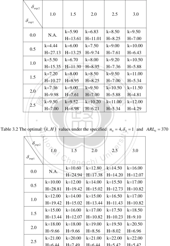
(18) <Step 1> Give parameters n0 , δ 3 , δ exp1 , δ exp 2 and ARL0 . <Step 2> Set the initial value of k equal to 2. <Step 3> Use the method described in section 3.2.3 to determine H. <Step 4> Use the k and H to minimize ARL1. <Step 5> Repeat Step 2 to Step 4 by stepwise increasing k with 0.01 until k reaches k max = 40 . <Step 6> Choose the best combination of (k, H ) that have the smallest ARL1.. 3.3 Numerical analyses for the optimal FP CUSUM Loss chart. 政治大. In reality, the expected shifts may not be equal the true shifts. Here, we set them in different. 立. shift scales. This section investigates the effects of parameters ( δ exp 1 , δ exp 2 , δ 1 , δ 2 , δ 3 ) on ARL1. ‧ 國. 學. for the optimal FP CUSUM Loss chart and X + S 2 charts under sampling time t 0 = 1 , sample. ‧. size n0 = 4 and ARL0 = 370 .. sit. y. Nat. First, build the optimal combination of (k, H ) under different combinations of δ exp 1 , δ exp 2. n. al. er. io. and δ 3 , then we can use it to further study later. The basic trend of k shows that when. i n U. v. δ exp 1 , δ exp 2 and δ 3 get larger, the k become larger. And the H goes contrary direction toward k.. Ch. engchi. The results are shown in Table 3.1 and Table 3.2.. 10.

(19) Table 3.1 The optimal (k, H ) values under the specified n0 = 4, δ 3 = 0 and ARL0 = 370. δ exp 2 1.0. 1.5. 2.0. 2.5. 3.0. δ exp 1 0.0. k=5.90 k=6.83 H=13.61 H=11.01. N.A.. k=8.50 H=8.25. k=9.50 H=7.00. k=4.44 k=6.00 k=7.50 H=27.13 H=13.25 H=9.74. k=9.00 H=7.61. k=10.00 H=6.43. 1.0. k=5.50 k=6.70 k=8.00 H=15.35 H=11.30 H=8.95. k=9.20 H=7.36. k=10.50 H=5.88. 1.5. k=7.20 k=8.00 H=10.27 H=8.95. k=8.50 H=8.25. k=11.00 H=5.34. 2.0. k=7.36 H=9.98. k=9.50 治政 H=7.00 大 k=9.00 k=9.50 k=10.50 H=7.61. H=7.00. H=5.88. k=11.50 H=4.81. k=9.52 H=6.98. k=10.20 H=6.21. k=11.00 H=5.34. 2.5. k=9.50 H=7.00. k=12.00 H=4.29. ‧. ‧ 國. 立. 學. 0.5. sit. n. al. 1.0. δ exp 1 0.0. Ch. N.A.. 1.5. 2.0. engchi U. er. io. δ exp 2. y. Nat. Table 3.2 The optimal (k, H ) values under the specified n0 = 4, δ 3 = 1 and ARL0 = 370. 2.5 v i n. 3.0. k=10.60 k=12.80 k=14.50 k=16.00 H=24.94 H=17.38 H=14.20 H=12.07. 0.5. k=10.00 k=12.00 k=14.00 k=15.50 k=17.00 H=28.81 H=19.42 H=15.02 H=12.73 H=10.82. 1.0. k=12.00 k=14.00 k=15.00 k=16.50 k=17.00 H=19.42 H=15.02 H=13.44 H=11.43 H=10.82. 1.5. k=15.00 k=16.00 k=17.00 k=17.50 k=18.50 H=13.44 H=12.07 H=10.82 H=10.23 H=9.10. 2.0. k=18.00 H=9.66. k=18.00 H=9.66. k=19.00 H=8.56. k=19.50 H=8.02. k=20.50 H=6.96. 2.5. k=21.00 H=6.44. k=20.00 H=7.49. k=21.00 H=6.44. k=22.00 H=5.42. k=22.00 H=5.42. 11.

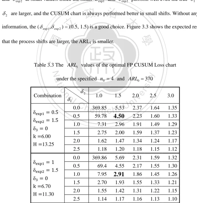
(20) Second, six optimal combinations of (k, H ) are chosen to compare under difference shift scales of δ 1 , δ 2 and δ 3 . Table 3.3 shows that when the expected process shifts ( δ exp1 , δ exp 2 ) equal the true process shifts ( δ 1 , δ 2 ), the ARL1 is the smallest. It is also the goal of the optimal FP CUSUM Loss chart. In reality, the true δ 1 and δ 2 are commonly unknown, so how to choose the δ exp 1 and δ exp 2 is a problem. Two solutions are recommended here. One is to choose the most possible δ exp 1 and δ exp 2 from historical data. Another is to choose the δ exp 1 and δ exp 2 at small values. Since the small δ exp 1 and δ exp 2 perform well even the true δ 1 and. 政治大. δ 2 are larger, and the CUSUM chart is always performed better in small shifts. Without any. 立. information, the ( δ exp1 , δ exp 2 ) = (0.5, 1.5) is a good choice. Figure 3.3 shows the expected result. ‧ 國. 學. that the process shifts are larger, the ARL1 is smaller.. ‧. Table 3.3 The ARL1 values of the optimal FP CUSUM Loss chart. y. Nat. n. δa1 l. δ2. δexp1 = 0.5 δexp2 = 1.5 δ3 = 0 k =6.00 H =13.25. δexp1 = 1 δexp2 = 1.5 δ3 = 0 k =6.70 H =11.30. Ch. 0.0. 1.0. 1.5. i U e369.85 n g c h5.53. er. io Combination. sit. under the specified n0 = 4 and ARL0 = 370. v ni 2.0. 2.5. 3.0. 2.37. 1.64. 1.35. 59.78. 4.50. 2.23. 1.60. 1.33. 1.0. 7.31. 2.96. 1.91. 1.49. 1.29. 1.5. 2.75. 2.00. 1.59. 1.37. 1.23. 2.0. 1.62. 1.47. 1.34. 1.24. 1.17. 2.5. 1.18. 1.20. 1.18. 1.15. 1.12. 0.0. 369.86. 5.69. 2.31. 1.59. 1.32. 0.5. 69.4. 4.55. 2.17. 1.55. 1.30. 1.0. 7.95. 2.91. 1.86. 1.45. 1.26. 1.5. 2.70. 1.93. 1.55. 1.33. 1.21. 2.0. 1.55. 1.42. 1.31. 1.22. 1.15. 2.5. 1.14. 1.17. 1.16. 1.13. 1.10. 0.5. 12.

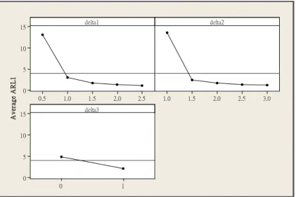
(21) δexp1 = 1.5 δexp2 = 1.5 δ3 = 0 k =8.00 H =8.95. δexp1 = 2 δexp2 = 2 δ3 = 0 k =9.50 H =7.00. 369.79. 6.24. 2.30. 1.56. 1.30. 0.5. 82.91. 4.85. 2.15. 1.52. 1.28. 1.0. 9.69. 2.96. 1.83. 1.43. 1.24. 1.5. 2.77. 1.90. 1.51. 1.31. 1.19. 2.0. 1.50. 1.39. 1.29. 1.20. 1.14. 2.5. 1.12. 1.15. 1.14. 1.12. 1.09. 0.0. 369.40. 6.89. 2.35. 1.56. 1.29. 0.5. 92.23. 5.27. 2.19. 1.52. 1.27. 1.0. 11.77. 3.10. 1.84. 1.42. 1.24. 1.5. 2.97. 1.93. 1.51. 1.30. 1.19. 2.0. 1.50. 1.38. 1.28. 1.20. 1.14. 2.5. 1.11. 1.14. 1.14. 1.12. 1.09. 2.23. 1.69. 1.89. 1.55. 0.0 0.5. 立1.0. 2.41. 1.91. 1.60. 1.41. 1.5. 1.81. 1.65. 1.50. 1.38. 1.29. 2.0. 1.27. 1.28. 1.26. 1.23. 1.19. 2.5. 1.05. 1.10. 1.12. 1.13. 1.12. 0.0. 370.05. 11.07. 3.61. 0.5. 16.67. 4.40. 2.52. 1.0. 3.42. 2.36. 1.84. 1.5. 1.72. 1.58. 1.45. a l2.0 2.5 Ch. 1.20. 1.23. 1.23. 1.03. 1.08. n. 1. 13. y. io. iv n1.10. e n gthecsmallest h i UARL Note : The bold figures represent match the true shifts.. 1.64. 1.55. 1.37. 1.34. 1.26. 1.20. 1.17. 1.11. 1.10. 2.16 1.83. 1.50. sit. Nat. δexp1 = 0.5 δexp2 = 2. er. ‧ 國. 3.30. ‧. δ3 = 1 k =12.00 H =19.42. 治10.15 3.60 政369.71 12.34 4.27 大2.57. 學. δexp1 = 0.5 δexp2 = 1.5. δ3 = 1 k =14.00 H =15.02. 0.0. when the expected shifts.

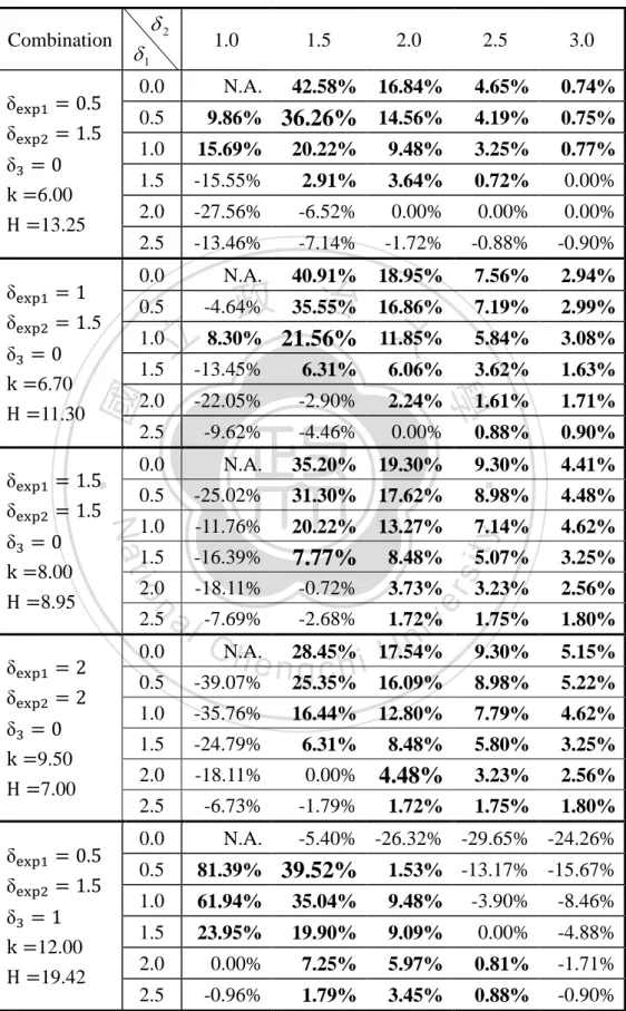
(22) delta1. 15. delta2. 10. Average ARL1. 5. 0 0.5. 1.0. 1.5. 2.0. 1.0. 2.5. 1.5. 2.0. 2.5. 3.0. delta3. 15. 10. 5. 0 0. 1. Figure 3.3 Main effects plot for δ 1 , δ 2 , δ 3 on ARL1 of the optimal FP CUSUM Loss chart. 政治大 The larger value of Saved立 Time indicates that the proposed optimal FP CUSUMC Loss. ‧ 國. 學. chart is more effective than X + S 2 charts. Table 3.4 shows the Saved Time of the proposed chart comparing to X + S 2 charts. On the whole, the optimal FP CUSUM Loss chart is better. ‧. than X + S 2 charts, but it may always fail in (1) Only process mean or variance has shifted,. sit. y. Nat. because the loss statistic consider both the process mean and variance, and the δ exp 1 and δ exp 2. er. io. are set up simultaneously. (2) The larger the difference between ( δ 1 and δ 2 ) and ( δ exp 1 and. al. n. v i n C hthe δ or δ is U ). Figure 3.4 also shows that when e n g c h i smaller, the Saved Time is larger,. δ exp 2. 1. 2. except the process variance hasn’t shifted (or δ 2 = 1 ).. 14.

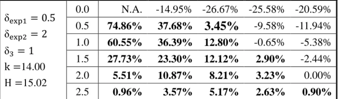
(23) Table 3.4 The Saved Time between the optimal FP CUSUM Loss chart and X + S 2 charts under specified n0 = 4 and ARL0 = 370. δ2. 0.74%. 14.56%. 4.19%. 0.75%. 1.0. 9.86% 36.26% 15.69% 20.22%. 9.48%. 3.25%. 0.77%. 1.5. -15.55%. 2.91%. 3.64%. 0.72%. 0.00%. 2.0. -27.56%. -6.52%. 0.00%. 0.00%. 0.00%. 2.5. -13.46%. -7.14%. -1.72%. -0.88%. -0.90%. 0.0. N.A.. 40.91%. 18.95%. 7.56%. 2.94%. 7.19%. 2.99%. 立 1.5 -13.45%. 5.84%. 3.08%. 6.31%. 6.06%. 3.62%. 1.63%. 2.0. -22.05%. -2.90%. 2.24%. 1.61%. 1.71%. 2.5. -9.62%. -4.46%. 0.00%. 0.88%. 0.90%. 0.0. N.A.. 35.20%. 19.30%. 9.30%. 4.41%. 0.5. -25.02%. 31.30%. 17.62%. 8.98%. 4.48%. 1.0. -11.76%. 20.22%. 13.27%. 7.14%. 1.5. -16.39%. 7.77%. 8.48%. -18.11%. -0.72%. 3.73%. -7.69%. -2.68%. 2.5. al. 0.0. CN.A. h e n28.45% gchi. y. 2.0. ‧. ‧ 國. 1.0. 4.62%. sit. 0.5. 學. δ3 = 1 k =12.00 H =19.42. 4.65%. n. δexp1 = 0.5 δexp2 = 1.5. 3.0. io. δ3 = 0 k =9.50 H =7.00. 16.84%. Nat. δexp1 = 2 δexp2 = 2. 42.58%. N.A.. 2.5. 治 16.86% -4.64% 政 35.55% 大 8.30% 21.56% 11.85%. δexp1 = 1 δexp2 = 1.5. δ3 = 0 k =8.00 H =8.95. 2.0. 0.5. δ3 = 0 k =6.00 H =13.25. δexp1 = 1.5 δexp2 = 1.5. 1.5. 0.0. δexp1 = 0.5 δexp2 = 1.5. δ3 = 0 k =6.70 H =11.30. 1.0. δ1. 5.07%. 3.25%. 3.23%. 2.56%. 1.75%. 1.80%. 9.30%. 5.15%. er. Combination. iv n 17.54% U 1.72%. 0.5. -39.07%. 25.35%. 16.09%. 8.98%. 5.22%. 1.0. -35.76%. 16.44%. 12.80%. 7.79%. 4.62%. 1.5. -24.79%. 6.31%. 8.48%. 5.80%. 3.25%. 2.0. -18.11%. 0.00%. 4.48%. 3.23%. 2.56%. 2.5. -6.73%. -1.79%. 1.72%. 1.75%. 1.80%. 0.0. N.A.. -5.40% -26.32% -29.65% -24.26% 1.53% -13.17% -15.67%. 1.0. 81.39% 39.52% 61.94% 35.04%. 9.48%. -3.90%. -8.46%. 1.5. 23.95%. 19.90%. 9.09%. 0.00%. -4.88%. 2.0. 0.00%. 7.25%. 5.97%. 0.81%. -1.71%. 2.5. -0.96%. 1.79%. 3.45%. 0.88%. -0.90%. 0.5. 15.

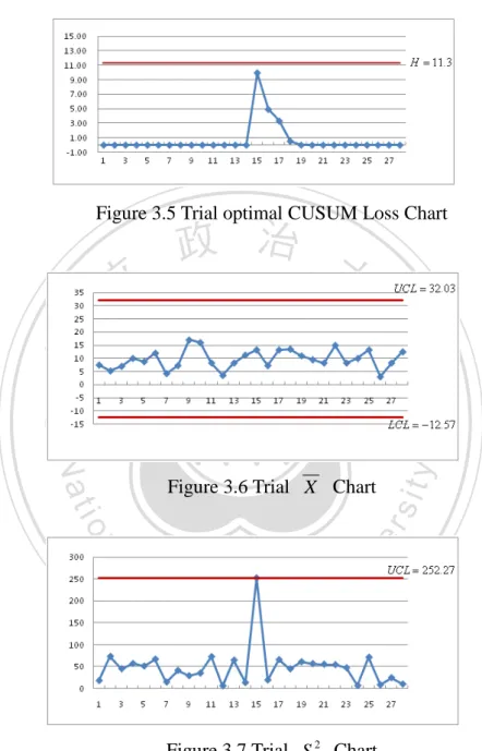
(24) δexp1 = 0.5 δexp2 = 2 δ3 = 1 k =14.00 H =15.02. 0.0. N.A.. -14.95% -26.67% -25.58% -20.59%. 0.5. 74.86%. 37.68%. 3.45%. -9.58% -11.94%. 1.0. 60.55%. 36.39%. 12.80%. -0.65%. -5.38%. 1.5. 27.73%. 23.30%. 12.12%. 2.90%. -2.44%. 2.0. 5.51%. 10.87%. 8.21%. 3.23%. 0.00%. 2.5. 0.96%. 3.57%. 5.17%. 2.63%. 0.90%. Note : The bold figures represent the positive Saved Time.. delta2. delta1. 0.16 0.12 0.08. Saved Tim e. 0.04 0.00 0.5 0.16. 立 1.0. 政治大. 1.5. 2.0. 2.5. 1.0. 1.5. 2.0. 2.5. 3.0. delta3. 0.12. ‧ 國. 學. 0.08 0.04 0.00. 1. ‧. 0. n. al. er. io. sit. y. Nat. Figure 3.4 Main effects plot for Saved Time of δ 1 , δ 2 , δ 3 comparing to X + S 2 charts. 3.4 Example for the optimal FP CUSUM Loss Chart. Ch. engchi. i n U. v. To show the application of the proposed optimal FP CUSUM Loss chart, this study uses the data from Braverman (1981). Data were obtained from 28 subgroups of size 4 and coded in 0.001 centimeter over 0.5 times 1000. This data is used to estimate the process mean and 2. 2 ˆ X= 9.73 , σˆ= variance µ= S= 48.42 , respectively.. Set ARL0 = 370 , δ exp 1 = 1, δ exp 2 = 1.5 , n0 = 4 and T = µˆ = 9.73 (or δ3 = 0 ) in this case. Based on Table 3.1, the optimal reference value k and upper control limit H of the optimal FP CUSUM Loss chart were (k , H ) = (6.7,11.3) . First, construct the trial optimal FP CUSUM Loss chart and X + S 2 charts to show whether 16.

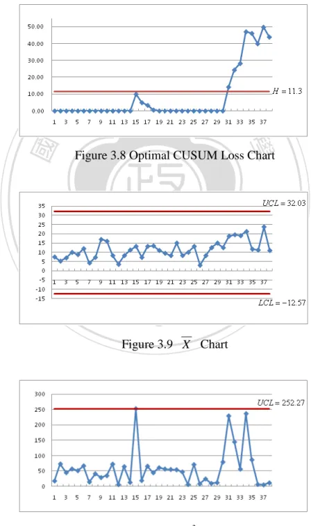
(25) the data is in control or not. Figure 3.5 to 3.7 show that no points fall outside of the optimal FP CUSUM Loss chart and X + S 2 charts, it indicates that all these charts can be used to monitor the following process.. Figure 3.5 Trial optimal CUSUM Loss Chart. 立. 政治大. ‧. ‧ 國. 學. n. er. io. al. sit. y. Nat. Figure 3.6 Trial X Chart. Ch. engchi. i n U. v. Figure 3.7 Trial S 2 Chart Next, use this optimal FP CUSUM Loss chart to monitor the following 10 out-of-control samples. The out-of-control data is randomly generated from normal distribution with mean ( µˆ + δ 1σˆ , δ 1 = 1 ) and variance ( δ 2σˆ 2 , δ 2 = 1.5 ) by Minitab 15.1. Figure 3.8 to 3.10 show that the optimal FP CUSUM Loss chart has a signal from the sample 31, but X + S 2 charts do not. So 17.

(26) the detection speed of the optimal FP CUSUM Loss chart is faster than X + S 2 charts in this case. The ARL1 of the optimal FP CUSUM Loss chart and X + S 2 charts are 2.91 and 3.71, respectively. The Saved Time comparing with X + S 2 charts is 21.56%. Hence, the optimal FP CUSUM Loss chart has better performance than X + S 2 charts.. 立. 政治大. ‧ 國. 學. Figure 3.8 Optimal CUSUM Loss Chart. ‧. n. er. io. sit. y. Nat. al. Ch. engchi. i n U. Figure 3.9 X Chart. Figure 3.10 S 2 Chart 18. v.

(27) 4. OPTIMAL VSI CUSUM LOSS CHART In general, an adaptive chart is more effective than a FP chart, so in this chapter, the Variable Sampling Interval feature is added and the optimal VSI CUSUM Loss chart is proposed. This chart uses the same statistic proposed in chapter 3 that can monitor the process mean and variance using a single chart. The following sections will show how to design this chart and how to find the optimal sampling intervals, the optimal reference value k, warning limit W and upper control limit H by numerical method and genetic algorithm. A numerical example is given to show how to implement the proposed optimal VSI CUSUM Loss chart and compare the. 政治大 optimal control parameters under 立different out-of-control situations, and compare the. detection speed with Shewhart X + S 2 charts. The numerical analyses show the results of the. ‧. ‧ 國. 學. performance with the optimal FP CUSUM Loss chart and Shewhart X + S 2 charts.. 4.1 Description of the optimal VSI CUSUM Loss chart. j =1. − T )2. , t = 1,2,.... al. n. n. sit. tj. io. L*t =. ∑(X. er. n. y. Nat. The statistic that represents the average quality loss. Ch. engchi U. (4.1). v ni. To standardize the statistic of the average quality loss, we can transform it into a new statistic Lt as follows Lt =. nL*t. σ2. , t = 1,2,.... (4.2). When the process is in control, Lt ~ χ n2,λ0 with the non-central chi square distribution of degrees of freedom n and non-central parameter λ0 = nδ 32 . When the process is out of control, Lt ~ δ 22 χ n2,λ1 , with the non-central chi square distribution of degrees of freedom n and non-central parameter λ1 = n((δ 1 + δ 3 ) / δ 2 ) . 2. This study considers the adaptive feature and proposes the optimal VSI CUSUM Loss chart. 19.

(28) Define the CUSUM statistic as follows C t = max(0, C t −1 + Lt − k ), t = 1,2,.... (4.3). where t is the sample number and k is the optimal reference value. Let the initial value C 0 = 0 . The optimal VSI CUSUM Loss chart can detect shifts in the process mean and/or variance by an abnormally large loss at the fastest speed with variable sampling interval and it issues an out-of-control signal at time t for which C t ≥ H , where H is a value of the optimal upper control limit with a given ATS0, W is a value of the warning control limit, and the lower control limit is zero because the CUSUM statistic here is only zero. 政治大 the location of the sample statistic 立on the proposed optimal VSI CUSUM Loss chart which. or greater. To express the relationship between the optimal sampling intervals t q , q = 1,2 and. ‧. ‧ 國. 學. consists three regions. See Figure 4.1.. I3. io. sit. y. Nat. UCLC = H. n. al. er. WCLC = W. Ch. LCLC = 0. engchi. i n U. v. I2 I1. Figure 4.1 The structure of the optimal VSI CUSUM Loss Chart. If the sample point C t falls within the interval I 1 , it is sampled after a long time interval ( t1 ). If the sample point C t falls within the interval I 2 , it is sampled after a short time interval ( t 2 ), where ( t1 > t 2 ). If the sample point C t falls within the interval I 3 , then the chart indicates an out-of-control signal. When t1 = t 2 = t 0 , the optimal VSI CUSUM Loss chart 20.

(29) becomes the optimal FP CUSUM Loss chart. The relationship between the next sampling interval and the position of the current sample statistics C t is expressed as follows. tq =. t1 , if C t ∈ I 1 t 2 , if C t ∈ I 2. 4.2 Design of the optimal VSI CUSUM Loss chart 4.2.1 The performance measurement. 政治大 an adaptive chart should have a large average time to signal when the process is in control and a 立 The average time to signal (ATS) of a chart represents the performance of a chart. Ideally,. small ATS when the process is out of control.. ‧ 國. 學. Define ATS 0 as the average time to signal when the process is in control, and ATS1 as. ‧. the average time to signal when the process is out of control.. sit. y. Nat. To compare the performance among the proposed optimal VSI CUSUM Loss chart, optimal. al. er. io. FP CUSUM Loss chart and X + S 2 charts, here define indices. v. ATS X + S 2 − ATSVSI ATS FP − ATSVSI × 100% ; Saved Time** = × 100% , ATS FP ATS X + S 2. n. Saved Time* =. Ch. engchi. i n U. where ATS FP denote as an ATS1 of the optimal FP CUSUM Loss chart, ATS X + S 2 denote as an ATS1 of X + S 2 charts, and ATSVSI denote as an ATS1 of the optimal VSI CUSUM Loss chart. The values of the Saved Time show that the proposed optimal VSI CUSUM Loss chart saves how much proportion of time in detecting process shifts comparing to the optimal VSI CUSUM Loss chart and X + S 2 charts while the process is out of control. When the values of the Saved Time are positive, it represents that the proposed optimal VSI CUSUM Loss chart has a better performance than the optimal FP CUSUM Loss chart and X + S 2 charts. 21.

(30) 4.2.2 ATS calculation based on Markov chain approach The approach to calculate the ATS of the proposed optimal VSI CUSUM Loss chart can be extended from the approach described in section 3.2.2. The following method shows the ATS calculation in detail. Divide the interval (0, H ) into N-1 subintervals with equal width 2d, where d =. H . 2( N − 1). Then let the interval (−∞,0] as the 1st subinterval and its midpoint m1 = 0 ; the interval (mi − d , mi + d ), i = 2,3,..., N as the i th subinterval, where mi =. (2i − 3) H . See Figure 4.2. 2( N − 1). Define the i th subinterval as the i th state. A state is said to be a transient state, if it can. 政治大. transfer to another states. A state is said to be an absorbing state, if it cannot transfer to another. 立. states. The state 1 to N are all transient states, because when a sample point falls within these. ‧ 國. 學. states, it indicates the process is in control, and the process keeps going. The action region above the control limit is defined as the N + 1th state that represents the absorbing state, because when. ‧. a sample point falls in the state, an out-of-control signal is given, and the process is stopped.. y. Nat. n. er. io. al. sit. Thus, the ATS is the expected time to absorption.. i n U. C hState N+1 = (H, ∞) engchi. v. H. State N = (H-2d, H) State N-1 = (H-4d, H-2d) ●●● ●●●. W. State 3 = (2d, 4d) State 2 = (0, 2d). 0. State 1 = (-∞, 0) Figure 4.2 States of the optimal VSI CUSUM Loss chart 22.

(31) The transition probability Pij is the probability of statistic C t −1 in state i at time t − 1 moving to state j at time t. That is the probability that C t lays in state j, conditioned on C t −1 being equal to the midpoint of the i th subinterval. Pi1 = P(C t ≤ 0 | C t −1 = mi ). = P(C t −1 + Lt − k ≤ 0 | C t −1 = mi ) = P(Lt ≤ −mi + k ). = Fχ 2. n ,λ. ((− m. i. (4.4). ). + k ) / δ 22 , i = 1,2,..., N , t = 1,2,3,.... Pij = P (m j − d ≤ C t < m j + d | C t −1 = mi ). = P (m j − d ≤ C t −1 + Lt − k < m j + d | C t −1 = mi ) = P (m j − mi − d + k ≤ Lt < m j − mi + d + k ) n ,λ. ((m. j. ). 政((m −治 m − d +大 k )/ δ. − mi + d + k ) / δ 22 − Fχ 2. 立. n ,λ. j. i. 2 2. ), i = 1,2,..., N , j ≠ 1, t = 1,2,3,... (4.5). 學. ‧ 國. = Fχ 2. where Fχ 2 (•) denote the cumulative non-central chi square distribution with degrees of n ,λ. ‧. freedom n and non-central parameter λ .. sit. y. Nat. Define P as a ( N + 1) × ( N + 1) transition probability matrix. Q be the matrix obtained from. n. al. er. io. P by deleting row N+1 and column N+1. In other words, Q = Pij , i, j = 1,..., N is the. transition probability matrix among the in-control states.. Ch. engchi. i n U. v. Denote b as the initial probability that the process started in state i, given that b = (b1 , b2 ,..., bN )' , where b1 = 1, bi = 0, ∀i ≠ 1 Denote t as the vector of sampling interval time for state 1 to state N, given that. t 2 , if W ≤ mi < H t = (t1∗ , t 2∗ ,..., t N∗ )' , i = 1,2,..., N , where t ∗i =  t1 , if 0 ≤ mi < W ,0 < t 2 < t1 < ∞ Thus, the ATS formula is ATS = b' (I − Q) −1 ⋅ t. (4.6). where I is the N × N identity matrix and 1 is a 1 × N column vector of ones. When the 23.

(32) process is in control, λ = λ0 , δ 1 = 0, δ 2 = 1 , Q=Q0 ; when the process is out of control,. λ = λ1 , δ 1 ≠ 0, δ 2 > 1 , Q=Q1 .. 4.2.3 Computing the warning control limit W under k and H To fairly compare the performance of the proposed optimal VSI CUSUM Loss chart with the optimal FP CUSUM Loss chart and X + S 2 charts, it is necessary to equalize their ATS0 to compute the warning control limit W under the constraint (4.7) ATS 0 = t 0 ⋅ ARL0 .. (4.7). When the n0 , t 0 , δ 3 , t1 , t 2 , k and H are determined, put them into the equation (4.8).. 政治大 f (n , t , δ , t , t , k , W , H ) = b' (I − Q ) ⋅ t = t ⋅ b' (I − Q ) 立 −1. 2. 0. 0. 3. 1. 2. 0. 0. −1. 0. ⋅1. (4.8). ‧ 國. 學. Then, using the dichotomy method in IMSL with subroutine “ZBREN” to solve the equation (4.8) in the range 0 < W < H .. ‧ sit. y. Nat. 4.2.4 The procedure of acquiring the optimal process parameters. n. al. er. io. This study uses a genetic algorithm to find the optimal combination of t1, t2 and k. Figure 4.3 shows the detail of this procedure.. Ch. engchi. 24. i n U. v.

(33) Randomly generate a group of variables t1, t2, k from uniform distribution. (Initial population=3000). Set the basic parameter values, such as n0 , t 0 , δ 3 , δ exp 1 , δ exp 2 , ATS 0. Input these random variables into the equations (3.12) and (4.8) to compute H and W.. Compute the ATS1 under the combination (t1 , t2, k, W, H). 立. To get better combination of t1, t2, k. Mutation 政治大. ‧ 國. 學. Crossover. Satisfy the terminal condition? (Generation=1000). No. ‧. Selection. sit. y. Nat. n. al. er. Yes. io. The procedures of selection, crossover, and mutation are necessary to obtain the best variable values and remove bad variable values. This approach iteratively improves the variable combinations.. Select the best combination of (t1, t2, k, W, H). Ch. engchi. i n U. v. Figure 4.3 The genetic algorithm procedure of the optimal VSI CUSUM Loss chart. 4.3 Numerical analyses for the optimal VSI CUSUM Loss chart This section investigates the effects of parameters ( δ 1 , δ 2 , δ 3 ) on ATS1 for the optimal VSI CUSUM Loss, optimal FP CUSUM Loss, and X + S 2 charts under t 0 = 1 , n0 = 4 , and ATS 0 = 370 . First, this study sets three levels of parameters of ( δ 1 , δ 2 , δ 3 ), taking δ 1 = (0.5, 1, 1.5), δ 2 =. 25.

(34) (1.5, 2, 2.5) and δ 3 = (0, 1, 1.5), and considers their 27 combinations in the analysis. Second, use the genetic algorithm to find the optimal combination of (t1 , t 2 , k , W , H ) in the range 1 < t1 ≤ 2 ,. 0.1 ≤ t 2 < 1 and 0 < k < 40 such that ATS1 is the smallest. The ATS1 and Saved times of the three charts are shown in Table 4.1. It also shows that the optimal value of t 2 always equal to 0.1 under different out-of-control situations, it indicates that the short sampling interval should be as short as possible. Use the Table 4.1 to make the main effects plots for δ 1 , δ 2 and δ 3 . Figure 4.4 indicates that when δ 1 or δ 2 is increasing, the average of ATS1 must be decreasing. Figure 4.5 and 4.6 show that when δ 1 and δ 2 are small, the proportion of the saved time is. 政治大 CUSUM Loss chart offers better 立performance than the optimal FP CUSUM Loss chart and higher than when δ 1 and δ 2 are large. This results show that the proposed optimal VSI. ‧. ‧ 國. 學. X + S 2 charts, especially when the shift scales are small.. n. er. io. sit. y. Nat. al. Ch. engchi. 26. i n U. v.

(35) Table 4.1 The ATSs and Saved times for the optimal VSI, FP CUSUM Loss charts and X + S 2 charts. 立. 政治大. ‧. ‧ 國. 學. n. er. io. sit. y. Nat. al. Ch. engchi. 27. i n U. v.

(36) delta1. delta2. 2.0 1.8. Average ATS1. 1.6 1.4 1.2 0.5. 1.0. 1.5. 1.5. 2.0. 2.5. delta3 2.0 1.8 1.6 1.4 1.2 0.0. 1.0. 1.5. Figure 4.4 The main effect plot for δ 1 , δ 2 , δ 3 on average ATS1 of the optimal VSI CUSUM Loss chart. 立. 政治大. delta2. delta1. 0.30. ‧ 國. 學. 0.25. 0.15 0.10 0.5. 1.0 delta3. 1.5. 0.0. 1.0. 1.5. 1.5. ‧. Saved Tim e*. 0.20. 2.0. 2.5. 0.30. y. Nat. 0.25. sit. 0.20 0.15. io. n. al. er. 0.10. Ch. Figure 4.5 The main effect plot for. engchi. i δ ,δ n ,δ U 1. 2. 3. v. on Saved Time*. delta2. delta1 0.45. Saved Tim e**. 0.40. 0.35. 0.30. 0.25. 0.20. 0.5. 1.0. 1.5. 1.5. 2.0. 2.5. Figure 4.6 The main effect plot for δ 1 , δ 2 , δ 3 on Saved Time** 28.

(37) 4.4 Example for the optimal VSI CUSUM Loss Chart To show the application of the proposed optimal VSI CUSUM Loss chart, this study uses 45 samples from Montgomery (2009) at p.232 and p.236. The experiments in this study formed samples using a hard-bake process in conjunction with the photolithography technique commonly used in semiconductor manufacturing. The first twenty-five samples, each including five wafers, represented the in-control process. We delete the 5th observation in each sample to have same sample size of four as FP CUSUM Loss chart. Then use this data set to estimate the process mean and variance. 政治大. µˆ = X = 1.491 , σˆ 2 = S 2 = 0.01765 , respectively.. 立. Set ATS 0 = 370 , δ exp 1 = 0.5, δ exp 2 = 1.5 , t 0 = 1 , n0 = 4 , and T = µˆ = 1.491 (or δ3 = 0 ). ‧ 國. 學. in this case. Based on Table 4.1, the optimal sampling intervals, reference value, warning control limit, and upper control limit of the optimal VSI CUSUM Loss chart were (t1 , t 2 , k , W , H ) =. ‧. (1.37, 0.1, 5.91, 0.271, 13.567).. y. Nat. sit. First, construct the trial optimal VSI CUSUM Loss chart and X + S 2 charts to show. n. al. er. io. whether the data is in control or not. Figure 4.7 to 4.9 show that no points fall outside of the. i n U. v. optimal VSI CUSUM Loss chart and X + S 2 charts, it indicates that all these charts can be used to monitor the following process.. Ch. engchi. Figure 4.7 Trial optimal VSI CUSUM Loss Chart 29.

(38) Figure 4.8 Trial X Chart. 立. 政治大. ‧. ‧ 國. 學. Nat. n. al. er. io. sit. y. Figure 4.9 Trial S 2 Chart. i n U. v. Next, use the optimal VSI CUSUM Loss chart to monitor the following out-of-control. Ch. engchi. samples. Twenty additional hard-bake wafer samples were collected after the trial control charts were established. Figure 4.10 to 4.12 show that the optimal VSI CUSUM Loss chart has a signal from the sample 41, but X + S 2 charts have a signal at sample 45. So the detection speed of the optimal VSI CUSUM Loss chart is faster than X + S 2 charts in this case. The out-of-control ATS of the optimal VSI CUSUM Loss chart, optimal FP CUSUM Loss chart and X + S 2 charts are 2.73, 4.50 and 7.06, respectively. The Saved Times comparing with the optimal FP CUSUM Loss chart was 39.44%, and comparing with the X + S 2 charts was 61.41%. Hence, the optimal VSI CUSUM Loss chart has much better performance than the optimal FP CUSUM Loss chart and X + S 2 charts. 30.

(39) Figure 4.10 Optimal VSI CUSUM Loss Chart. 立. 政治大. ‧. ‧ 國. 學 Figure 4.11 X Chart. n. er. io. sit. y. Nat. al. Ch. engchi. i n U. Figure 4.12 S 2 Chart. 31. v.

(40) 5. OPTIMAL VSSI CUSUM LOSS CHART In this chapter, both Variable Sample Size and Variable Sampling Interval are added to this chart, and the optimal VSSI CUSUM Loss chart is proposed. This chart transforms the average quality loss statistic proposed in chapter 3 into a normal distribution by the normal approximation which was proposed by Patnaik in 1949. Because the non-central chi square distribution changes its degrees of freedom under variable sample size feature, it makes the reference value and warning control limit must be changed with difference sample size. It is too difficult to implement, so this study uses the normal approximation to exclude the effects of. 政治大 into a normal distribution, how立 to design this chart and how to find the optimal sample sizes,. degrees of freedom. The following sections will show how to transform the average quality loss. ‧ 國. 學. sampling intervals, optimal reference value k, warning control limit W and upper control limit H by numerical method and genetic algorithm. A numerical example is given to show how to. ‧. implement the proposed optimal VSSI CUSUM Loss chart and compare the detection speed with. sit. y. Nat. CUSUM X + S 2 charts and Shewhart X + S 2 charts with variable sample size. The numerical. n. al. er. io. analyses show the results of the optimal process parameters under different out-of-control. i n U. v. situations, and compare the performance with the optimal VSI CUSUM Loss chart, optimal FP. Ch. engchi. CUSUM Loss chart, CUSUM X + S 2 charts and Shewhart X + S 2 charts.. 5.1 Description of the optimal VSSI CUSUM Loss chart The statistic that represents the average quality loss nq. L = * t. ∑(X j =1. tj. nq. − T )2 ~. σ 2 χ n2 ,λ q. nq. , t = 1,2,.... (5.1). where χ n2q ,λ denote the non-central chi-square distribution with degrees of freedom nq and non-central parameter λ = nq ((δ 1 + δ 3 ) / δ 2 ) . 2. 32.

(41) Patnaik (1949) proposed two normal approximation approaches of the non-central chi-square distribution. From simulation results, the equation (5.2) is a better normal approximation even n is small.. 2(n + λ )χ n2,λ n + 2λ. 2(n + λ ) − 1 ≈ N (0,1) n + 2λ 2. −. (5.2). Using the above result, the statistic of average quality loss is transformed into a new statistic Lt as follows. Lt =. (. ). 2nq 1 + δ 32 L*t. (1 + 2δ )σ 2 3. 2. (. 2nq 1 + δ 32. −. 1 + 2δ 32. ). 2. −1. 政治大 When the process is out of control or X~N (μ + δ σ,δ σ ) , the statistic L ≈ N (µ , σ ) 立 δ (1 + δ )(2n (1 + δ ) − (1 + 2δ )) − (1 + δ )(2n (1 + δ ) − (1 + 2δ )) where µ = 1. 2 2 c. q. t. 2 c. (1 + δ )(1 + 2δ ) 2 c. δ + δ3 δ 22 (1 + δ 32 )(1 + 2δ c2 ) and δ c = 1 2 2 δ2 (1 + δ c )(1 + 2δ 3 ). 2 3. 2 c. q. 2 2 3. 2 1. 1. 2 3. ‧. σ 12 =. ‧ 國. 1. 2 3. 2. 學. 2 2. 2 2. (5.3). Nat. sit. er. io. Appendix shows the detail.. y. When the process is in control (or δ1 = 0 and δ 2 = 1 ), the statistic is reduced to Lt ≈ N (0,1) .. al. n. v i n C hfeature and proposesUthe optimal VSSI CUSUM Loss This study considers the adaptive engchi. chart. Define the CUSUM statistic as follows C t = max(0, C t −1 + Lt − k ), t = 1,2,.... (5.4). where t is the sample number and k is the optimal reference value. Let the initial value C 0 = 0 . The optimal VSSI CUSUM Loss chart detects shifts in the process mean and/or variance by an abnormally large loss at the fastest speed with variable sample size and sampling interval and it issues an out-of-control signal at time t for which C t ≥ H , where H is a value of the optimal upper control limit with a given ATS0, W is a value of the warning. control limit, and the lower control limit is zero because the CUSUM statistic here is only zero 33.

(42) or greater. To express the relationship between the optimal sample sizes, nq , q = 1,2 , sampling intervals t q , q = 1,2 , and the location of the sample statistic on the proposed optimal VSSI CUSUM chart which consists three regions. See Figure 5.1.. I3. UCLC = H. I2. WCLC = W. LCLC = 0. 立. 政治大. I1. ‧ 國. 學. Figure 5.1 The structure of the optimal VSSI CUSUM Loss Chart. ‧. If the sample point Ct falls within the interval I1 , the next sample should be small ( n1 ),. sit. y. Nat. io. er. sampled after a long time interval ( t1 ). If the sample point Ct falls within the interval I 2 , the. al. next sample should be large ( n2 ), sampled after a short time interval ( t 2 ), where ( n1 < n2 , t 2 < t1 ).. n. v i n C U chart indicates an out-of-control falls within thehinterval e n gIc,htheni the. If the sample point Ct. 3. signal. When n1 = n2 = n0 , the proposed optimal VSSI CUSUM Loss chart becomes the optimal VSI CUSUM Loss chart. When n1 = n2 = n0 and t1 = t 2 = t 0 , the proposed optimal VSSI CUSUM Loss chart becomes the optimal FP CUSUM Loss chart. The relationship among the next sample size, sampling interval and the position of the current sample statistics C t is expressed as follows. (n. q. , tq ) =. (n1 , t1 ), if L ∈ I 1 (n2 , t 2 ), if L ∈ I 2. 34.

(43) 5.2 Design of the optimal VSSI CUSUM Loss chart 5.2.1 The performance measurement The average time to signal of a chart represents the performance of a chart. Ideally, an adaptive chart should have a large average time to signal when the process is in control and a small ATS when the process is out of control. The average number of observations to signal is known as the ANOS. It can be used to measure the sampling cost of a chart. Define ATS 0 as the average time to signal when the process is in control, ATS1 as the average time to signal when the process is out of control, ANOS 0 as the average number of. 政治大 observations to signal when the立 process is out of control.. observations to signal when the process is in control, ANOS1 as the average number of. ‧ 國. 學. To compare the performance among the proposed optimal VSSI CUSUM Loss chart, optimal FP CUSUM Loss chart and X + S 2 charts, here define indices. ‧. Saved Time* =. sit. n. al. er. ANOS X + S 2 − ANOSVSSI ANOS FP − ANOSVSSI × 100% ; Saved ANOS** = × 100% , ANOS FP ANOS X + S 2. io. Saved ANOS* =. y. Nat. ATS X + S 2 − ATSVSSI ATS FP − ATSVSSI × 100% ; Saved Time** = × 100% ATS FP ATS X + S 2. Ch. engchi. i n U. v. where ATS FP and ANOS FP denote as an ATS1 and ANOS1 of the optimal FP CUSUM Loss chart, ATS X + S 2 and ANOS X + S 2 denote as an ATS1 and ANOS1 of X + S 2 charts, and ATSVSSI and ANOSVSSI denote as an ATS1 and ANOS1 of the optimal VSSI CUSUM Loss chart. The values of the Saved Time show that the proposed optimal VSSI CUSUM Loss chart saves how much proportion of time comparing to the other two charts while the process is out of control, and the values of the Saved ANOS show that the proposed optimal VSSI CUSUM Loss chart save how much proportion of sampling cost comparing to the other two charts while the process is out of control.. 35.

(44) 5.2.2 ATS and ANOS calculations based on Markov chain approach The approach to calculate the ATS and ANOS of the proposed optimal VSSI CUSUM Loss chart can be extended from the approach described in section 3.2.2. The following method shows the ATS and ANOS calculations in detail. Divide the interval (0, H ) into N-1 subintervals with equal width 2d, where d =. H . 2( N − 1). Then let the interval (−∞,0] as the 1st subinterval and its midpoint m1 = 0 ; the interval (mi − d , mi + d ), i = 2,3,..., N as the i th subinterval, where mi =. (2i − 3) H . See Figure 5.2. 2( N − 1). Define the i th subinterval as the i th state. A state is said to be a transient state, if it can. 政治大. transfer to another states. A state is said to be an absorbing state, if it cannot transfer to another. 立. states. The state 1 to N are all transient states, because when a sample point falls within these. ‧ 國. 學. states, it indicates the process is in control, and the process keeps going. The action region above the control limit is defined as the N + 1th state that represents the absorbing state, because when. ‧. a sample point falls in the state, an out-of-control signal is given, and the process is stopped.. y. Nat. n. al. er. io. observations to absorption.. sit. Thus, the ATS is the expected time to absorption and ANOS is the expected number of. i n U. C hState N+1 = (H, ∞) engchi. v. H. State N = (H-2d, H) State N-1 = (H-4d, H-2d) ●●● ●●●. W. State 3 = (2d, 4d) State 2 = (0, 2d). 0. State 1 = (-∞, 0) Figure 5.2 States of the optimal VSSI CUSUM Loss chart 36.

(45) The transition probability Pij is the probability of statistic C t −1 in state i at time t − 1 moving to state j at time t. That is the probability that C t lays in state j, conditioned on C t −1 being equal to the midpoint of the i th subinterval. Pi1 = P(C t ≤ 0 | C t −1 = mi ). = P(C t −1 + Lt − k ≤ 0 | C t −1 = mi ). (5.5). = P(Lt ≤ −mi + k ). = Φ ((− mi + k − µ1 ) / σ 1 ), i = 1,2,..., N , t = 1,2,3,... Pij = P (m j − d ≤ C t < m j + d | C t −1 = mi ). = P (m j − d ≤ C t −1 + Lt − k < m j + d | C t −1 = mi ) = P (m j − mi − d + k ≤ Lt < m j − mi + d + k ). = Φ ((m j − mi + d + k − µ1 ) / σ 1 ) − Φ ((m j − mi − d + k − µ1 ) / σ 1 ), i = 1,2,..., N , j ≠ 1, t = 1,2,3,.... 政治大. (. (5.6). ). 2. (1 + δ )(1 + 2δ ) 2 3. ). y. sit. n. al. Define P as a ( N + 1) × ( N + 1). er. io. n1 , if 0 ≤ mi < W. n2 , if W ≤ mi < H. 2. ‧. 2 c. Nat. And nq =. (. δ 22 (1 + δ 32 ) 2nq (1 + δ c2 ) − (1 + 2δ c2 ) − (1 + δ c2 ) 2nq (1 + δ 32 ) − (1 + 2δ 32 ). δ1 + δ 3 δ 22 (1 + δ 32 )(1 + 2δ c2 ) = δ and σ = c δ2 (1 + δ c2 )(1 + 2δ 32 ) 2 1. 學. where µ1 =. ‧ 國. 立. i n C U h e nprobability transition g c h i matrix.. v. Q be the matrix obtained from. P by deleting row N+1 and column N+1. In other words, Q = Pij , i, j = 1,..., N is the. transition probability matrix among the in-control states. Denote b as the initial probability that the process started in state i, given that b = (b1 , b2 ,..., bN )' , where b1 = 1, bi = 0, ∀i ≠ 1 Denote t as the vector of sampling interval time for state 1 to state N, given that. t1 , if 0 ≤ mi < W t = (t1∗ , t 2∗ ,..., t N∗ )' , where t ∗i =  t 2 , if W ≤ mi < H ,0 < t 2 < t1 < ∞ 37.

(46) Denote n as the vector of sample size for state 1 to state N, given that. n1 , if 0 ≤ mi < W n = (n1∗ , n2∗ ,..., n N∗ )' , where n ∗i =  n2 , if W ≤ mi < H ,0 < n1 < n2 < ∞ Thus, the ATS and ANOS formulas are ATS = b' (I − Q) −1 ⋅ t. (5.7). ANOS = b' (I − Q) −1 ⋅ n. (5.8). where I is a N × N identity matrix. When the process in in-control, δ 1 = 0, δ 2 = 1 , Q=Q0; when the process is out-of-control, δ 1 ≠ 0, δ 2 > 1 , Q=Q1.. 立. 政治大. 5.2.3 Computing the warning control limit W under k and H. ‧ 國. 學. To fairly compare the performance of the proposed optimal VSSI CUSUM Loss chart with. ‧. the optimal FP CUSUM Loss chart and X + S 2 charts, it is necessary to equalize their ATS0. Nat. n. al. (5.9). er. io. ANOS 0 = n0 ⋅ ARL0 .. sit. using the constraint (5.9) to compute the warning control limit W.. y. and ANOS0. Because the sample size must be positive integer, we first equalize the ANOS0 by. i n U. v. When the n0 , δ 3 , n1 , n2 , k and H are determined, put them into the equation (5.10).. Ch. engchi. f 3 (n0 , δ 3 , n1 , n 2 , k , W , H ) = b' (I − Q 0 ) −1 ⋅ n = n0 ⋅ b' (I − Q 0 ) −1 ⋅ 1. (5.10). Then, using the dichotomy method in IMSL with subroutine “ZBREN” to solve the equation (5.10) in the range 0 < W < H .. 5.2.4 Computing the long sampling interval t1 The dependant variable t1 can be solved by equalizing the ATS0 as follows. ATS 0 = t 0 ⋅ ARL0 .. (5.11). When the t 0 , δ 3 , n1 , n2 , t1 , k , W and H are determined, put them into the equation (5.12). 38.

(47) f 4 (t 0 , δ 3 , n1 , n 2 , t1 , t 2 , k , W , H ) = b' (I − Q 0 ) −1 ⋅ t = t 0 ⋅ b' (I − Q 0 ) −1 ⋅ 1. (5.12). Then, using the dichotomy method in IMSL with subroutine “ZBREN” to solve the equation (5.12) in the range 0 < t1 < t max = 2 .. 5.2.5 The procedure of acquiring the optimal process parameters This study uses the following steps to design the optimal VSSI CUSUM Loss chart in detecting δ 1 ≠ 0 and δ 2 > 1 . Figure 5.3 shows the detail of this procedure.. 0. ‧ 國. 立. Set the basic parameter values, 政治大 such as n , t , δ , δ , δ , ARL 3. exp 1. exp 2. 0. ‧. Input these random variables into the equations (3.12), (5.10) and (5.12) to compute H, W, t1. To get better combination of n1, n2, t2, k. n. er. io. sit. y. Nat. al. 0. 學. Randomly generate a group of variables n1, n2, t2, k from uniform distribution (Initial population=5000). Ch. Compute the ATS1 under the combination (n1, n2, t1 , t2, k, W, H). i n U. v. Mutation. engchi. Crossover. Satisfy the terminal condition? (Generation=5000). No Selection. The procedures of selection, crossover, and mutation are necessary to obtain the best variable values and remove bad variable values. This approach iteratively improves the variable combinations.. Yes Select the best combination of (n1, n2, t1 , t2, k, W, H). Figure 5.3 The genetic algorithm procedure of the optimal VSSI CUSUM Loss chart 39.

(48) 5.3 Numerical analyses for the optimal VSSI CUSUM Loss chart This section investigates the effects of parameters ( δ 1 , δ 2 , δ 3 ) on ATS1 and ANOS1 for the optimal VSSI CUSUM Loss, optimal FP CUSUM Loss, and X + S 2 charts under t 0 = 1 , n0 = 4 and ATS 0 = 370 . First, this study sets three levels of parameters ( δ 1 , δ 2 , δ 3 ), taking δ 1 = (0.5, 1, 1.5), δ 2 = (1.5, 2, 2.5) and δ 3 = (0, 1, 1.5), and considers their 27 combinations in the analysis. Second, use the genetic algorithm to find the optimal combination of (n1 , n2 , t1 , t 2 , k , W , H ) in the range. 2 ≤ n1 ≤ 3 , 5 ≤ n2 ≤ 20 , 1 < t1 ≤ 2 , 0.1 ≤ t 2 < 1 and 0 < k < 40 such that ATS1 is the smallest.. 政治大. The ATS1, ANOS1 and Saved times of the three charts are shown in Table 5.1. It shows that the. 立. optimal value of n1 always equal to 3 and the optimal value of t 2 always nearly equal to 0.1. ‧ 國. 學. under different out-of-control situations, it indicates that the small sample size should be as small as possible and the short sampling interval should be as short as possible. Use the Table 5.1 to. ‧. make the main effects plots for δ 1 , δ 2 and δ 3 . Figure 5.4 and 5.5 indicate that when δ 1 or δ 2. y. Nat. io. sit. is increasing, the average of ATS1 and ANOS1 must be decreasing, but when δ 3 is increasing,. er. the average of ATS1 and ANOS1 are slightly increasing. Figure 5.6 to 5.9 show that when δ 1. al. n. v i n are small, the proportion ofCthe saved times are higher than when hengchi U. and δ 2. δ 1 and δ 2 are large.. This results show that the proposed optimal VSSI CUSUM Loss chart offers better performance than the optimal FP CUSUM Loss chart and X + S 2 charts, especially when the shifts are small.. 40.

(49) Table 5.1 The ATSs, ANOSs and Saved times for the optimal VSSI, FP CUSUM Loss charts and X + S 2 charts. 立. 政治大. ‧. ‧ 國. 學. n. er. io. sit. y. Nat. al. Ch. engchi. 41. i n U. v.

(50) delta1. 2.0. delta2. 1.8. Average ATS1. 1.6 1.4 0.5. 1.0. 1.5. 1.5. 2.0. 2.5. delta3. 2.0 1.8 1.6 1.4 0.0. 1.0. 1.5. Figure 5.4 The main effect plot for δ 1 , δ 2 , δ 3 on average ATS1 of the optimal VSSI CUSUM Loss chart. 14. 立. 政治大. delta1. delta2. 10. 0.5. 1.0. 1.5. 1.5. 2.0. 2.5. delta3. 14. ‧. Average ANOS1. 學. ‧ 國. 12. 12. Nat. 0.0. 1.0. sit. y. 10. 1.5. er. io. Figure 5.5 The main effect plot for δ 1 , δ 2 , δ 3 on average ANOS1. n. aoflthe optimal VSSI CUSUM Loss v chart i n Ch engchi U delta2. delta1 0.30 0.25 0.20. Saved Tim e*. 0.15 0.10 0.5. 1.0 delta3. 1.5. 0.0. 1.0. 1.5. 1.5. 2.0. 2.5. 0.30 0.25 0.20 0.15 0.10. Figure 5.6 The main effect plot for δ 1 , δ 2 , δ 3 on Saved Time*. 42.

(51) delta2. delta1 -0.20 -0.24 -0.28. Saved ANOS*. -0.32 -0.36 0.5. 1.0 delta3. 1.5. 0.0. 1.0. 1.5. 1.5. 2.0. 2.5. -0.20 -0.24 -0.28 -0.32 -0.36. Figure 5.7 The main effect plot for δ 1 , δ 2 , δ 3 on Saved ANOS*. 政治大 delta2. delta1 0.5. 0.3. 0.2. ‧. 0.1 1.0. 1.5. 1.5. 2.0. 2.5. y. Nat. 0.5. sit. ‧ 國. 立. 學. Saved Tim e**. 0.4. io. n. al. er. Figure 5.8 The main effect plot for δ 1 , δ 2 , δ 3 on Saved Time**. Ch. engchi. delta1. 0.10. i n U. v. delta2. Saved ANOS**. 0.05 0.00 -0.05 -0.10 -0.15 -0.20 -0.25 0.5. 1.0. 1.5. 1.5. 2.0. 2.5. Figure 5.9 The main effect plot for δ 1 , δ 2 , δ 3 on Saved ANOS**. 43.

(52) 5.4 Example for the optimal VSSI CUSUM Loss Chart To show the application of the proposed optimal VSSI CUSUM Loss chart, this study uses the data from DeVor, Cheng, and Sutherland (1992) at p.186 and p.187. The quality characteristic is the outside diameter of a motor shaft, which has a nominal value of 2.125 inches and a tolerance of ±0.001 inch. The data collected occurred in samples of five consecutive parts. The measurements are in inches and to the nearest ten-thousandth of an inch (e.g. 2.1248 and 2.1259 inches, etc.). The data are coded using the last two digits. This study varies the sample size and arranges the raw data in a single row, then samples from the single raw data. The. 政治大. in-control process mean µˆ = X = 48.79 and variance σˆ 2 = S 2 = 41.81 are estimated. 立. respectively from historical data.. ‧ 國. 學. Set ATS 0 = 370 , δ exp 1 = 0.5, δ exp 2 = 1.5 , t 0 = 1 , n0 = 4 , and T = µˆ = 41.81 (or δ3 = 0 ) in this case. Based on Table 5.1, the optimal sample sizes, sampling intervals, reference value,. ‧. warning control limit, and upper control limit of the optimal VSSI CUSUM Loss chart were. sit. y. Nat. (n1 , n2 , t1 , t 2 , k ,W , H ) =(3, 10, 1,15, 0.11, 0.96, 0.27, 2.27).. n. al. er. io. Use the optimal VSSI CUSUM Loss chart to monitor the data. Figure 5.10 to 5.12 show. i n U. v. that the optimal VSSI CUSUM Loss chart has a signal from the sample 19, while Standardized. Ch. engchi. X Chart with variable sample size has a signal at sample 21. So the detection speed of the. optimal VSSI CUSUM Loss chart is faster than X + S 2 charts with variable sample size in this case. To compare the detection speed between the optimal VSSI CUSUM Loss chart, optimal VSI CUSUM Loss chart, optimal FP CUSUM Loss chart, CUSUM X + S 2 charts and X + S 2 charts, this study lets δ1 = 0.5, δ2 = 1.5, and uses a computer program to calculate the ATS1 and Saved Time. See Table 5.2.. 44.