以分界特徵限制為基礎之即時道路邊緣追蹤演算法

國

立 交 通 大 學

生醫工程研究所

碩 士 論 文

以分界特徵限制為基礎之即時

道路邊緣追蹤演算法

A New Method of Efficient Road Following

Algorithm Based on Temporal Region Ratio and

Edge Constraint

研 究 生：陳宣輯

指導教授：林進燈 博士

中華民國 九十八 年 六 月

以分界特徵限制為基礎之即時道路邊緣追蹤演算法

A New Method of Efficient Road Boundary Tracking Algorithm

Based on Temporal Region Ratio and Edge Constraint

研 究 生：陳宣輯 Student：Shen-Chi Chen

指導教授：林進燈 博士

Advisor：Dr. Chin-Teng Lin

國立交通大學

資訊工程學院

生醫工程研究所

碩士論文

A Thesis

Submitted to Institute of Biomedical Engineering

College of Computer Science

National Chiao Tung University

in Partial Fulfillment of the Requirements

for the Degree of Master

in

Computer Science

June 2009

Hsinchu, Taiwan

以分界特徵限制為基礎之即時

道路邊緣追蹤演算法

學生：陳宣輯

指導教授：林進燈 博士

國立交通大學資訊工程學院生醫工程研究所

Chinese Abstract

中文摘要

近年來隨著車輛數目的增加與性能不斷的成長，道路情況與駕車難度也相對 的提升，當今的車輛仍需要駕駛者全神貫注地人為操作，相對地增加駕駛人的壓 力與車禍發生的可能性。隨著行車安全愈來愈受到人們重視，為了改善此問題， 世界各國的研究機構、知名車廠、學術研究室均投入大量的精力於智慧型運輸系 統ITS(Intelligent Transportation System) 中的安全駕駛輔助系統，並得到許多人 的期待與讚許。也因此這類的先進式車輛控制系統的願景，以從當初的駕駛者安 全輔助性質轉為主動式的安全操縱系統，甚至最終的目標已經設定為自動駕駛。 行駛道路邊緣的偵測為其中一項關鍵的技術，本論文將以 CCD (charge coupled device)攝影機所擷取的影像為基礎利用本論文提出的邊緣特徵穩定地實現道路 邊緣偵測與追蹤的演算法。 本研究所提出的道路邊緣特徵結合了邊緣強度與道路顏色兩項重要的特 徵，改進了當今許多研究只利用其中一類可能會產生的問題。我們將在論文中說 明如何利用所提出的創新演算法修正其他文獻的問題。本研究的演算法利用有效 的特徵，增加系統之適應性，可處理多類型的道路邊緣，包括一般市區道路、高 速公路、等有明顯車道線的邊緣；另外，由於我們所採用的邊界特徵擁有突出的 穩定性與一致性；因此本系統對於一些鄉間小路、產業道路..等，沒有明顯的標 線邊緣，與夜間道路仍能提供有效性地偵測結果。本系統在設計時在考慮許多駕 駛狀況，因此，系統具有處理一般駕駛狀況與道路環境的改變的能力，如變換車

道，左右偏動，與不平坦道路，造成相機的晃動。本篇論文提出一主車道邊緣偵 側與追蹤系統，其具有先進的適應性與即時的處理效率。

A New Method of Efficient Road Boundary

Tracking Algorithm Based on Temporal Region

Ratio and Edge Constraint

Student: Shen-Chi Chen

Advisor: Dr. Chin-Teng Lin

Institute of Biomedical Engineering

College of Computer Science

National Chiao Tung University

English Abstract

Abstract

In recent years, since the number and properties of the vehicle are continuous increasing, the complexity of road condition and the difficulties of operation increase relatively. As of today, physically driving not only requires drivers’ full attention but could potentially amplify drivers’ stress and possibility of car accidents. As people become more concerned about the safety in driving, many research institutes around the world, well-known automobile manufactures, and academic research labs invest a tremendous amount of effort to develop a safe driving assistance system of ITS (Intelligent Transportation System) to alleviate the problems of physical driving. With many expectation and applaud, the advanced supporting system has transformed into an active safe operating system, and ultimately will develop into an automatic driving system. Since the driving path boundary detection is one of the key techniques of automatic driving system, this paper is based on the use of images captured by the CCD (charge coupled device) camera and we discovered the general boundary features to steadily achieve main driving path boundary detection and tracking

system.

We purpose to integrate two major features, edge intensity and color distribution, of road boundary and mitigate the problems encountered by many other studies which utilize only one major feature for road boundary detection. In this paper we will explain how to make use of the advanced algorithms to amend the problems in other literatures. Our algorithms utilize effective features to enhance the adaptability of the system; the system is able to manage various types of road boundary includes general urban road, highway, or any boundary with the clear lane line. In addition, we use the general characteristics of the boundary, and therefore the system is still able to effectively provide detection result at the road without clear boundary such as the countryside paths, the road with no lane line, and the scene at the night. In the design of the system we take into account many driving situations, such as changing lanes, left and right side move, and non-flat roads lead to camera shake. Therefore, the system possesses good ability to deal with general driving conditions and variations. This paper presents a system which includes main driving path boundary detection and boundary tracking with advanced real-time adaptability and efficiency.

Chinese Acknowledgements

致 謝

本論文的完成，首先要感謝指導教授林進燈博士與蒲鶴章博士、范剛 維博士這兩年來的悉心指導，讓我學習到許多寶貴的知識，在學業及研究 方法上也受益良多。另外也要感謝口試委員們的的建議與指教，使得本論 文更為完整。 其次，感謝超視覺驗室的子貴、建霆、琳達、肇廷、明峰與東霖所有 的學長與學姐細心地指導，與同學 哲銓、鎮宇與耿維的相互砥礪，一起 奮鬥一起歡樂，也感謝學弟們在研究過程中所給我的鼓勵與協助。其中我 的大貴人子貴學長，在理論及程式技巧上給予我相當多的幫助與建議，讓 我獲益良多。另外也感謝學弟多次辛苦地幫助我拍攝行車影片，建立了許 多寶貴的資料庫。這兩年讓我在學問與處事經驗成長很多，感恩之情，永 藏於心，希望未來仍有機會為實驗室貢獻自己小小的力量。 感謝我的父母親對我的教育與栽培，並給予我精神及物質上的一切支 援，使我能安心地致力於學業。此外也感謝妹妹對我不斷的關心與鼓勵。 謹以本論文獻給我的家人及所有關心我的師長與朋友們，我永遠愛你們。

Contents

Chinese Abstract ...ii

English Abstract ...iv

Chinese Acknowledgements ...vi

Contents ...vii List of Tables...ix List of Figures...x Chapter 1 Introduction...1 1.1 Background...1 1.2 Motivation...4 1.3 Objective ...5 1.4 Organization...6

Chapter 2 Relate Works ...7

2.1 Overview...7

2.2 Approaches Introduction...7

Chapter 3 Proposed Techniques ...21

3.1 Objective ...21

3.2 On-lined L*a*b color model...21

3.2.1 Objective..………...21

3.2.2 Color space selection………..22

3.2.3 On-lined Model………...26

3.3 LMR boundary window...36

3.3.1 Overview……….36

3.3.2 LMR boundary window introduction………..37

3.3.3 Boundary feature of LMR boundary window……….38

Chapter 4 System Algorithm...42

4.1 Overview...42

4.2 Driving Path Boundary Detection...43

4.2.1 Objective……….43

4.2.2 Methods………..44

4.3 Boundary Tracking Algorithm ...51

4.3.2 The Alignment of LMR Boundary Window ………...53

Chapter 5 Experimental Results...67

5.1 Experimental Results of Driving Path Boundary Detection...67

5.2 Experimental Results of Boundary Tracking...69

Chapter 6 Conclusion ...73

6.1 Contribution ...74

6.2 Future Works...76

List of Tables

Table 1 : Traffic accident and violation in Taiwan from 2002 to 2006...2 Table 2 : Related research organization of intelligent transportation system ...2

List of Figures

Fig. 1-1: The Blind Spot Information System (BLIS) [Volvo] ...3

Fig. 1-2: Adaptive Cruise Control System (ACC) ...3

Fig. 1-3: Volvo’s City Safety System [Volvo]...3

Fig. 1-4: The most popular sensors are used in driver assistant systems...5

Fig. 2-1: The most popular features...8

Fig. 2-2: The disadvantages of common features. ...9

Fig. 2-3: Detection result by region based approach and our desired resluts. ...10

Fig. 2-4: Instability of the region-based methods without adaptive module. ...10

Fig. 2-5: The feature and common disadvantages of the region based methods. ...13

Fig. 2-6: The method using bird-viewed image by IPM transform ...14

Fig. 2-7: The difficult reasons of boundary based approach...14

Fig. 2-8: Points transfer to (θ,γ) plane. ...16

Fig. 2-9: Extract the boundaries with maximal accumulator values...16

Fig. 2-10: Edge feature encounter difficult problems ...17

Fig. 2-11: The feature and common disadvantages of the boundary based methods ..17

Fig. 2-12: Spline model to describe the boundary by the control points P1 P2 P3...18

Fig. 2-13: The position Xm divides the scene into far field and near field. ...19

Fig. 2-14: The lane-curve function (LCF) and its asymptotes...19

Fig. 2-15: The feature and common disadvantages of the model based methods ...20

Fig. 3-1: The max-min value of L*a*b values...24

Fig. 3-2: The comparison results using L*a*b color space and HSV color space...25

Fig. 3-3: On-lined learning procedure. ...27

Fig. 3-4: Guide snake keep tracking the curvature oft the road...28

Fig. 3-5: LMR boundary window is set as ROI s. Guide Snake make LMR boundary window have its exclusive sampling area...28

Fig. 3-6: Blob noises appear in experimental videos...32

Fig. 3-7: Filtering the blob noises...32

Fig. 3-8: A color ball i in the L*a*b color model...33

Fig. 3-9: Each color ball hold a weight record...34

Fig. 3-10: The pixel matched with first B weight color balls as the standard color. ...36

Fig. 3-11: Introduction LMR boundary window ...38

Fig. 3-12: The characteristic of the boundary...39

Fig. 3-13: Guide snake set the nearest area as exclusive sampling ...41

Fig. 3-14: The boundary resides on the one of the block in LMR boundary cause the maximum boundary energy on that block. ...41

Fig. 4-2: There are several common challenges in boundary detection...43

Fig. 4-3: The flow chart of Driving Path Boundary Detection ...44

Fig. 4-4: The procedure of edge-based approach...45

Fig. 4-5: Comparison between with de-noise and without it ...45

Fig. 4-6: Gaussian filter to de-noise...46

Fig. 4-7: The result of each step of the edge-based approach...48

Fig. 4-8: The problem of boundary detection by edge feature method...49

Fig. 4-9: Modified boundary detection methods...50

Fig. 4-10: The result of the modified boundary detection methods...51

Fig. 4-11: Primary overview of boundary tracking...52

Fig. 4-12: The boundary tracking algorithm in the system architecture...52

Fig. 4-13: The flow chart of alignment of LMR boundary window. ...53

Fig. 4-14: The boundary features appear or disappear in LMR boundary windows. ..54

Fig. 4-15: Checking the accumulator window to process the boundary alignment (optimization). Alternatively, it will process boundary detection (searching)...55

Fig. 4-16: The steps of boundary alignment (optimization) ...58

Fig. 4-17: Checking the accumulator window and then Performs the boundary detection procedure...59

Fig. 4-18: (a): The boundary is broken line so it detects no boundary appear in the searching range. (b): The LMR boundary will remain at original position and wait for the incoming segment of the broken line...61

Fig. 4-19: (a): The boundary have deviated the range of LMR boundary window, so the accumulator window detected no boundary trace. (b): The LMR boundary tracks the last boundary position in the searching range and aligns to it. ...62

Fig. 4-20: (a): L block with the maximum boundary; (b): LMR boundary move toward left side to align to boundary. The correct alignment regress the region ratio, both RoadPower and NonRoadPower, to previous effective range. ...64

Fig. 4-21: (a): The boundary alignment to left is in error because the fake edge resulted from the prominent shadow. (b): After the wrong alignment, the incorrect position of LMR boundary window can be checked by the NonRoadPower of Region Ratio Feature shown in green block. ...65

Fig. 4-22: (a): The boundary alignment to right is in error because the fake edge resulted from the object outside path. (b): After the wrong alignment, the incorrect position of LMR boundary window can be checked by the RoadPower of Region Ratio Feature shown in green block. ...66

Fig. 5-1: The tested vehicle...67

Fig. 5-2: Experimental results of driving boundary detection. ...69

Fig. 5-4: Experimental results of change line situation. ...72 Fig. 6-1: The main features and disadvantages of region-based methods. Our

algorithm can modify and solve the problems...75 Fig. 6-2: The main features and disadvantages of boundary-based methods. Our algorithm can modify and solve the problems...75

1

Chapter 1

Introduction

1.1 Background

In recent year, the number of higher performance vehicle is growing up and causes more problem of traffic safety. As seen in Table 1, the traffic safety is worse and worse in the statistics about the road traffic accident and violation in Taiwan from 2002 to 2009. Therefore, Intelligent Transportation System (ITS) has been preceded for many years. Intelligent conveyance system ITS (intelligent transportation system) integrates with the advance technology of application in many field including computer, electronics, communication science etc. It promotes transportation system of security, efficiency, comfort, and reduces the confusion of road environment.

Duo to the reason of safety requirement of consumers, it attracts a lot of car manufactories, research institution and laboratories to engage in this research area. In this new generation, the intelligent transportation system has been developed rising and flourish as seen in Table 2. ITS has develop to many sub-areas such as Advanced Traffic Management Systems (ATMS), Advanced Traveler Information System (ATIS), Advanced Vehicle Control and Safety Systems (AVCSS), Commercial Vehicle Operations (CVO), Advanced Public Transportation System (APTS), Advanced Rural Transportation System (ARTS). In ITS America of USA, it includes seven sub-systems and among of those items the most important development is the advanced vehicle control and safety system AVCSS. In the same way Europe and Japan all make a lot of effort to study in AVCSS.

Table 1 : Traffic accident and violation in Taiwan from 2002 to 2006 [20].

Related research organization of intelligent transportation system Car Manufactories GM (Tahoe Boss), Land Rover(Land-E), Ford,

Honda, Toyota, Nissan Research Institution

US Defense Department,

CSIST, ITRI, ARTC, MIRDC

(Taiwan Automotive Research Consortium, TARC) Research Laboratories CMU (Navlab), Stanford (AI lab)

Table 2: Related research organization of intelligent transportation system The Advanced Driver Assistance System (ADAS) has become an important component in AVCSS research area of Intelligent Transportation System (ITS). From the beginning, the researchers just hope to design a robust system which can help driver to avoid some dangerous occurrence by giving an alarm in time. Along with the progress of technology, the functions of driver assistance system are more powerful and more reliable. The Active Driving Safety System or Autonomous Guided Vehicles (AGV) has become a popular research field in the area of intelligent Transportation System.

Many advanced driver assistance products have published and promoted. The advance driver assistances include Blind Spot Information System (BLIS), Adaptive Cruise Control (ACC), Obstacle Detection, City Safety System, etc shown in Fig. 1-1, Fig. 1-2, and Fig. 1-3 [21].Among these assistant systems, the fundamental technique is road following system, and main driving boundary detection is especially important Year 2002 2003 2004 2005 2006 Number of accident 86307 120223 137221 155812 160897 Number of Deaths 2861 2718 2634 2894 2734 Number of Injuries 109612 156303 179108 203087 204187

to realize the driving condition around the vehicle.

Fig. 1-1: The Blind Spot Information System (BLIS) [Volvo]

Fig. 1-2: Adaptive Cruise Control System (ACC)

1.2 Motivation

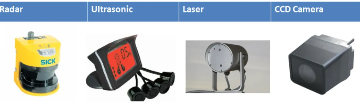
There are various sensors which can be exploited to capture useful features to develop different technologies in ITS research area. The tools such like radar, laser scanner, ultrasonic, CCD camera etc have been used on autonomous vehicles to detect the passable road and sense the surrounding environment. These sensors have some characteristic which appropriate to process specific function. The radar and laser scanner are usually used to detect obstacle on the road. Radar is more robust than laser in the rain or in the mist; however the cost of radar is more expensive. The ultrasonic can not work as long as laser scanner but it still helps to detect near obstacle on the lateral of vehicle. The radar, laser and ultrasonic are classified to the active sensor because they deliver the signal by themselves and estimation the distance with the obstacle using the reflective signal. The main disadvantage of active sensor is the limit of scan speed and without accurate distance estimated with obstacle. The CCD camera is another type of sensor which is called passive sensor. Due to the progressive performance of computer system, the camera becomes a common sensor in driver-assistance system.

In the AGV system, the road detection and road following is the principal element because it verifies vehicle position on the roadway and it is to support automatic navigation or curvature estimation. As a result, road following and road detection techniques have been extensively developed due to their widely applications in the Intelligent Transport System (ITS) and other similar researching fields in the past decades. The CCD camera has some prominent advantages such as the capability of acquiring abundant road information in a non-invasive way and with cheaper way to realize the road detection and road following. The most important reason is that the

active sensor can not handle the road detection and road following requirement. As a result, the vision-based road following system is a significant research area and critical component of AGV system.

Fig. 1-4: The most popular sensors are used in driver assistant systems

1.3 Objective

In the thesis, it is proposed a vision-based efficient road following algorithm. Since 1980s, road following become a widely studied field in computer vision. Although many methods have existed to handle the road detection or road following problem, these method are demonstrably limited by various assumption of the ideal condition in order to simplify the task of road following. Most of researchers focus their works on structured road, on which clear marks can be recognized or without sharply curve. Therefore the approach proposed attempts to deal most condition of road. It is presented a novel approach based on the general feature of the boundaries regardless of encountering unstructured roads, unclear road edges, non-homogeneous road appearance, arbitrary road shape and be adaptive automatically to resist interferences such as paint covered on the road or variations of lightness especially from shadows.

1.4 Organization

This thesis is organized as follows. In the next chapter, we briefly review the related topic papers then describe methods and discuss the most features which they adopted. In chapter 3, the proposed core techniques in this system are described in detail. They modify the inadequacy and disadvantage of the features. In chapter4, the main algorithm is presented. In chapter 5, we will show the experimental results and have a discussion on efficiency and reliability of proposed algorithm. Finally, the conclusions of our algorithm and future work will be presented in chapter 6.

2

Chapter 2

Relate Works

2.1 Overview

In recent years, many researchers have developed many techniques for road and driving situation detection in the frontal view of vehicle. The related topics to our research include “road detection”, “road recognition”, “road following”, and “lane detection” etc. In this chapter, these related works are classified by the reason that they used different approaches or different features. Furthermore, we will describe the problems which might be happened in the real condition. In section 2.2, it divides the existed methods into several bases by the features which are adopted to extract the positions of boundaries or roads and then we briefly introduce these methods.

2.2 Approaches Introduction

To distinguish the roads and boundaries for driving situation detection in the frontal view of vehicle, many researchers have proposed diverse approaches which depend on different bases and using different features. We describe the most important bases which include “region-based”, “boundary-based”, and “model-based” and introduce briefly the most popular features.

The most common features can be divided into four typical types as seen in Fig. 2-1. The methods usually utilize one or integrate different features to realize the frontal situation of vehicle during driving.

Fig. 2-1: The most popular features.

The first feature selection to detect road area is applying color information. There is some unstableness of color feature. The common causes of these unstableness including non-homogeneous surface or light variation. It is important that the method using color feature can adapt the color setting simultaneously. However, the color feature method cannot capture the precise road area and compute current road information adaptively. Furthermore, the speed of processing is time-consuming because color images require three times data quantity than the grey-scale images.

The second feature selection is to locate road boundary using edge characteristics of the boundary. If there is no distinct boundary features, or non-boundary objects may produce stronger edge intensity, all of these reasons may mistakenly lead to false detection. The third feature selection is to utilize the geometry of the road. Geometric feature largely depends on vanish line information, but camera shaking encountered during driving will destabilize the position of the vanish line in the image. On the other hand, many approaches adopt inverse perspective mapping (IPM) to transform the original image to bird-viewed image. Bird-viewed images are capable to

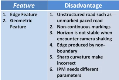
capture the parallel characteristic of the road boundary; but many adjustments of parameters such as the placement of the camera and internal camera information are required. Finally, the last feature, texture selection, encountered the same drawback as the color feature. Besides, since most road surface is smooth, it is hard to discriminate the drive way from the whole surrounding. We have summarized the overall disadvantages of common features in the Fig. 2-2.

Fig. 2-2: The disadvantages of common features.

The universal approaches which can be divided to three kinds of bases are “region-based”, “boundary-based”, and “model-based”. We introduce the main idea of these methods as follows:

1. Region-Based :

The methods with topics about road detection or road recognition usually belong to region-based. The idea of region-based is like the solution of segmentation problems. Region-based methods adopt road features to extract the road region. The features include the color features and texture features and many methods use these

features to identify if the pixel or the region is the road or non-road. However, the road detection methods usually identify the approximate road region as seen in Fig. 2-3. Actually, the ultimate goal is to detect the boundary of the main drive path. Some methods combine the edge and geometric features about the boundary and shape of the road to estimate the candidate road regions firstly and narrow the search area from the whole image to the candidate regions in order to save the detection time.

(a) (b) (c)

Fig. 2-3: (a) captured image, (b) road detection result, (c) the boundary of the main drive path.

The region based methods usually catch the key point on color or texture information between road region and non-road region, and apply the clustering algorithm by these features. They design a threshold or hyper-plane such as decision boundary to identify which category region or a single pixel is. Such region based methods are usually insensitive to road shapes, but sensitive to illumination variation and inconsistent surface such as shadows and non-homogeneous appearance as seen in Fig. 2-4.

Fig. 2-4: The non-homogeneous appearance of surface causes instability of the region-based without adaptive module.

The supervised classification applied to road following (SCARF) [1] and unsupervised clustering applied to road following system (UNSCARF) [12] are integrated with navigation system at NAVLAB of Carnegie Mellon University (CMU). The system can deal with unstructured in urban without obvious lane marking but with considerable difference in color between road area and surroundings. They are considered as a method of color segmentation based on clustering. The SCARF uses the RGB as color features to build multiple Gaussian color models in road/non road area and using standard nearest mean clustering (K-means) to cluster the pixels into four classes for each road and non-road with similar colors. The UNSCARF adopt iterative self-organizing data-analysis technique algorithm (ISODATA) to cluster a pixel x with five-dimensional as feature extracted by RGB color space and the coordinate of the pixel x in the image such as x = [R, G, B, X, Y]. These methods using the clustering technique have to process iteratively to fit the best clustering result but the steps are too time-consuming to meet the real-time requirement. In addition, they are difficult to distinguish the road from its surroundings only by color for the similar color or road area and the area that is beyond road shoulder. Furthermore, they assumed the width of road is known and the road is linear so the road recognition result is less accurate when the curvature of road is sharp and the width of road is non-uniform. As a result, they display its inability to detect arbitrary road shapes explicitly.

J.Huang 2007 [3] uses HSV color space to detect the unstructured road without priori knowledge. It just assumes a small area in front of the vehicle as a sample of road to compute means of Hue, color purity defined as Saturation multiplied by Value of HSV color space and judge a whether a pixel belongs to the road or not by the simple Manhattan distance measure with the means of color purity. The color of road

is grayish, and RGB is similar value. Therefore, the Hue component is always sensitive and unstable, but color purity composed of Saturation and Value components is not enough discriminative from road and non-road. In addition, the method belongs to the pixels based so the processing time is slow. Because they do not use any edge information of boundary, so the effectiveness of the approach is not stable. Mobileye [4] designed an autonomous driving vehicle for Darpa Grad Challenge Race in the Mojave desert. They adopted Adaboost learning principle based on the texture information of the road which is extracted by oriented filter, Walsh-Hadamard kernels and Moment to detect the off-road path. The approach is only appropriate to the surface with uniform texture on the off-road path. However, this method often fails when current road is dissimilar to that of the training set. Rasmussen [5] utilized the texture cue to navigate the vehicle on the unstructured road which is without any lane markings and a homogeneous surface. Previous approaches use color feature to build a Gaussian mixture models [6][7] but the color on the road is actual not homogenous. Road colors are different produced by the reasons including: different light, different material of surface etc, so the color model is not adaptive enough to perform precisely. Some methods proposed the learning model [8], but they don’t have methods to define where the road regions are. Therefore, the samples to build the model are not appropriate and the reason why the effective of learning become even worst.

We have summarized the overall features selected and common disadvantages of the region-based approaches in the Fig. 2-5.

Fig. 2-5: The feature and common disadvantages of the region based methods.

2. Boundary Based :

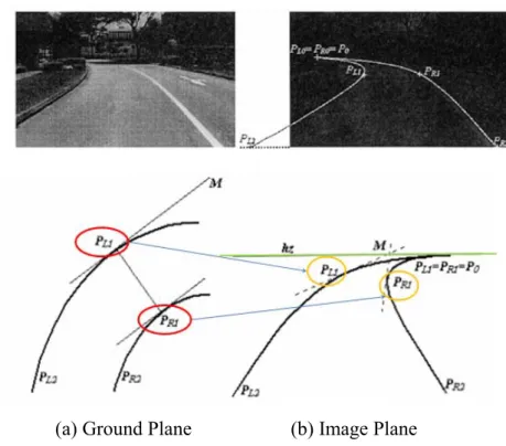
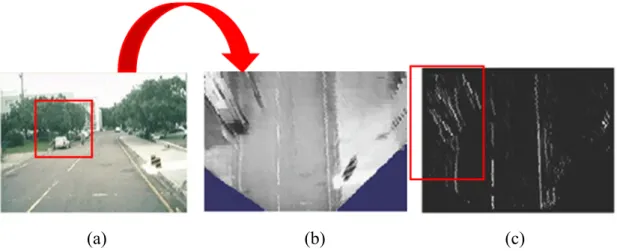
Some methods use the characteristic includes edge and shape of the roadside to extract the boundary position. Bertozzi et al. [10] proposed the GOLD (Generic Obstacle and Lane Detection) system by using a stereo vision-based hardware and software architecture developed to increment road safety of moving vehicles. The GOLD system addresses both lane detection and obstacle detection at the same time. Lane detection is a boundary based skill which relies on the presence of road marking, while the localization of obstacles in front of the vehicle is performed by the processing of pairs of stereo images. The IPM (Inverse Perspective Mapping) [11] is the most important component. The IPM algorithm can be used to project image plane to ground plane which is assumed to be z=0 in the real world as shown a bird-viewed scene shown in Fig. 2-6 (a) to (c). Meanwhile, road boundaries become parallel two lines in the bird-viewed image and extract the boundaries by the hint. However, the IPM algorithm needs appropriate parameters of the camera setting information so it is not compatible enough to use immediately after setting on the vehicle. Besides, some objects may produce edge as interference as seen in Fig. 2-6 (c), it cause difficulties of the detection.

(a) (b) (c)

Fig. 2-6: The method transform to bird-viewed image using inverse perspective mapping (a) to (b) and extract the boundaries from bird-viewed image (b) to (c)

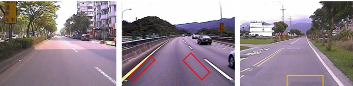
Most of the boundary based approaches [10][12][13][14] rely on the distinctness of the boundary, such methods assume a clear and solid lane mark on the surface of the road. The ambiguous country roadside or the broken lane mark in the middle of the road could lead to the failure in following the detection of main drive path shown in Fig. 2-7 (a) and (b). The shadow or objects at the side of the road could sometimes render the strong edge information as seen Fig. 2-7 (b) and (c); such interferences need to be avoided in order to precisely detect the road boundary.

(a) (b) (c)

Fig. 2-7: The difficult reasons of boundary based approach.

In order to increase the accuracy, some methods usually combine the edge feature with geometric properties of the road [10][12][13]. Due to the perspective

sin cos x θ+y θ γ=

effect of camera, each pair of parallel lines in the real world would connect to the vanish point on the horizon in the captured image. Generally, the key of the approach is to use voting procedure such as Hough transform for the edge points of the image to the (θ,γ) plane by equationand (2-1) and form a sinusoidal curve in (θ,γ) plane as seen Fig. 2-8 (a) and (b) .

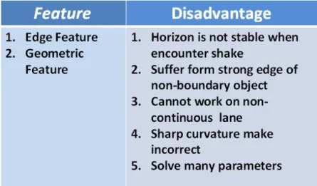
(2-1) They divide the image to many sections and compute the accumulator values after all edge points have been transformed to the (θ,γ) plane. It detect the pair of boundaries by extracting the pair of line with maximal accumulator and intersecting on the vanish line as seen in Fig. 2-9. These algorithms are fast and appropriate for the task of highway driving; however, it make assumptions about the structure of the road, and do not work on the unmarked roads without clear and distinct lanes on the boundaries. They have great problem by the effect on the edges of the surrounding objects, so it always is not acceptable when the road is too narrow to extract enough edge of boundaries. In addition, the camera which is set on the vehicle is shaked due to flatness of road when the vehicle is moving. As a result , the vanish line position is not stable which cause the algorithm to extract the incorrect boundaries. In addition, these approaches could not detect precisely when the road curvature is very sharp, because the boundary in the far field sections is unclear and the strong edges prodiced by the objects around surroundings make the curve boundary detection failed as shown Fig. 2-10. Therefore, the height of far field section must be decresed to handle the sharp curve boundary.

We have summarized the overall features selected and common disadvantages of the boundary-based approaches in the Fig. 2-10.

(a) (b) Fig. 2-8: Points transfer to (θ,γ) plane.

Fig. 2-9: Extract the boundaries in each section by selecting the lines with maximal accumulator values [12].

Fig. 2-10: It is suffered from edges of non road boundary and difficult to detect the curve boundary precisely

Fig. 2-11: The feature and common disadvantages of the boundary based methods

3. Model Based

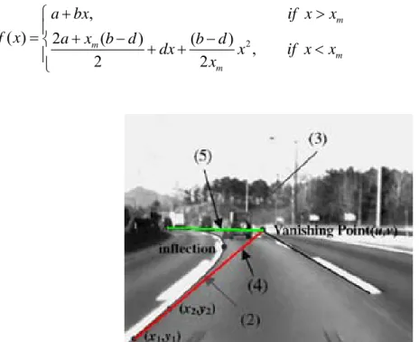
The last method is the model based. They apply the mathematic function to model the road boundary shape. They use the some feature such as edge and geometric feature to converge to model to the boundary position and minimize its divergence errors. [12][13] Wang use a local interpolating spline such like

Catmull-Rom Spline and B-Spline to describe the boundary shape by setting the control points on the boundary shown in Fig. 2-12. Jung 2005 [14] utilized the edge feature and then combined edge distribution function and modified Hough transform to locate the boundary first and then used a linear-parabolic model to perform lane following and lane departure detection. The linear-parabolic model use linear equation to track the near field boundary, and then use quadratic equation to track the far field. The near field and far field is shown in Fig. 2-13 and the linear-parabolic mode is as equation (2-2). The same idea is adopted in [15] and they use vanish point and the control points on the boundary to model their lane-curve function (LCF) shown in Fig. 2-14.

(a) Ground Plane (b) Image Plane

Fig. 2-13: The position Xm divides the scene into far field and near field. 2 , ( ) 2 ( ) ( ) , 2 2 m m m m a bx if x x f x a x b d b d dx x if x x x + > ⎧ ⎪ =⎨ + − _{+ +} − _< ⎪⎩ (2-2)

Fig. 2-14: The lane-curve function (LCF) and its asymptotes. (2) is the near field LCF, (3) is the far field LCF, (4) is the near field asymptote, and (5) is the far field asymptote.

Actually, the model based approach relies on the accuracy of the feature. If the feature is unstable, the model cannot converge to the precise position of the boundary. Moreover, if the shape of the boundary is too twisted, the first and second degree equation cannot match the curve. Multiple curves of the road could also complicate the parameters of the formula. We summarize all the common features of model based method and its disadvantage in the below Fig. 2-15.

3

Chapter 3

Proposed Techniques

3.1 Objective

The last chapter two has introduced current approaches using different bases including region based, boundary based, and model based. Besides we have realized frequent inadequacy of the features they adopt. Therefore, we proposed the two core techniques in this chapter in order to promote the precision and plasticity of the road following system. The two main core techniques are: 1. On-lined L*a*b color model and 2. LMR boundary window. The first technique attempts to train the adaptive color model and modify the non-homogeneous drawback of the road color. The second technique uses a new tracking tool called LMR boundary window to extract boundary position by edge intensity difference. We introduce the details of the core techniques and explain how they can solve the inadequacy of the features.

3.2 On-lined L*a*b color model

3.2.1 Objective

Most region based approaches frequently use the color feature to detect the road. Color information extends into three times dimensions of original grey scale image so it is with better discrimination. Therefore, there will be results in a more completed and precise detection. Most current papers propose off line method to determine the ranges of each color vector. This method only enables the detection of road area

within the color range. However, off-line method is very ineffective because of the difficulty to cope with the heterogeneity of surface material and the variation of illumination. Therefore, we purpose an on-line learning model that allows continuously update during driving. Through the training method, we can enhance plasticity of the system.

Besides, due to the uneven distribution of the road color, we select the samples which most closely resemble the detection zone to build the exclusive color model. In addition, we don’t detect the whole image but set the each LMR boundary windows which prepare to track the boundary position as the region of interesting (ROI). Therefore, when we track the boundary we just detect each LMR boundary window (ROI) in order to increase the detection speed and the performance of updating models. Besides, each LMR boundary window has exclusive color model whose on-lined sampling area is very close to its corresponding LMR boundary window. The exclusive model and its adequate sampling area can promote detection accuracy in each LMR boundary window when the road surface with uniform color appearance.

3.2.2 Color space selection

In this section, we illustrate the advantaged properties of L*a*b color space by comparing the other color space and explain the reason we adopt the L*a*b color feature for modeling.

We attempt to describe the color appearance in the driving environment by selecting the color features and using these color features to build a color model of the road, therefore we have to choose a color space which has uniform, little correlation, concentrated properties in order to increase the accuracy of the model. In computer color vision, all visible colors are represented by vectors in a three-dimensional color

space. There are many common color spaces that have been used to facilitate the analysis of color image.

Among all the different color spaces, RGB color space is the most common color feature selected because it is the initial format of the captured image without any distortion. Using the RGB color space to build model had been seen in many approaches [16]. However, the RGB color feature is high correlative, and the similar colors spread extensively in the color space. As a result, it is difficult to evaluate the similarity of two color from their 1-norm or Euclidean distance in the color space.

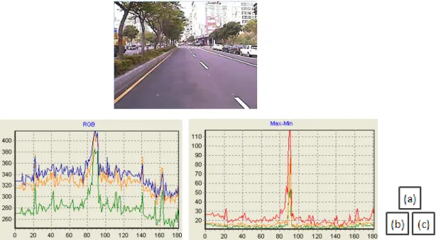
It takes some experimental results to explain the L*a*b color space is a better choice than others. RGB color space is susceptible to illumination variation on the road such as shadow. In Fig. 3-1, we track the values of (Imax-Imin) of each component on a selected road area over time which distribute at the horizontal axis using both RGB and L*a*b. We can see the RGB is greatly interfered by the shadow which leads to the values (Imax-Imin) of each component in the road area fluctuate drastically. On the contrary, the (Imax-Imin) of L*a*b is quite stable around the value of 0 to 30 intensity at the vertical axis except during the time interval from 80th to 100th frames. Fig. 3-1, the peak during the time 80th to 100th frames is resulted from a plaint on the road.

Fig. 3-1: The captured video (a). The max-min value of each three components of RGB at the vertical axis distribute around the frame sequence at the horizontal axis (b) and same as L*a*b (c). It is obvious that the L*a*b is more stable.

.

The other standard color space HSV is supposed to be closer to the way of human color perception. Both HSV and L*a*b resist to the interference of illumination variation such as the shadow when modeling the road area. However, the performance of HSV model is not as good as L*a*b model because the road color cause the HSV model not uniform lead to the HSV color model not as uniform as the L*a*b color model. There are many reasons attribute this result. Firstly, HSV is very sensitive and unstable when lightness is low. Furthermore, the Hue is computed by dividing (Imax - Imin) in which Imax = max(R,G,B), Imin = min(R,G,B), therefore when a

pixel has a similar value of Red, Green and Blue components, the Hue of the pixel may be undetermined. Unfortunately, most of the road surface is in similar gray colors with very close R, G, and B values. If using HSV color space to build road color model, the sensitive variation and fluctuation of Hue will generate inconsistent road colors and decrease the accuracy and effectiveness.

L*a*b* color space is based on data-driven human perception research that assumes the human visual system owing to its uniform, little correlation, concentrate characteristics are ideally developed for processing natural scenes and is popular for color-processed rendering [17]. L*a*b* color space also possesses these characteristics to satisfy our requirement. It maps similar colors to the reference color with about the same differences by Euclidean distances measure and demonstrates more concentrated color distribution than others. As a result, we will compare with BGR and HSV through experimental result.

We compare the detection results between L*a*b and HSV color space in the Fig. 3-2. First of all, L*a*b is more sensitive toward the grayish color than the HSV color space, so it can yield a better result in road detection. Secondly, due to the concentration property of L*a*b color space, it can use fewer and less spread Gaussian models to express overall road scenery. As a result, the method using L*a*b color space takes less time for road detection.

:

0.431 0.342 0.178 X = ⋅ +R ⋅ +G ⋅B 0.222 0.707 0.071 Y = ⋅ +R ⋅ +G ⋅B 0.020 0.130 0.939 Z = ⋅ +R ⋅ +G ⋅B / n 0.008856 if Y Y ≤ * 500 [ ( / _n) ( / )]_n a = ⋅ f X X − f Y Y 1/3 * 903.3 [ / ]_n L = ⋅Y Y * 200 [ ( / )_n ( / _n)] b = ⋅ f Y Y −f Z Z 1/3 _{/ 0.008856} ( ) 7.787 16 /116 / 0.008856 n n t Y Y f x t Y Y ⎧ > ⎪ = ⎨ + ≤ ⎪⎩

The RGB-L*a*b conversion is described as follow equations: 1. RGB-XYZ conversion: (1) (2) (3) 2. Cube-root transformation: 1/3 * 166 [ / ]_n 16 L = ⋅Y Y − if Y Y/ n >0.008856 (4) (5) (6) Where Xn, Yn, Zn, are XYZ tristimulus values of reference white point, and Xn=95.05,

Yn=100, Zn=108.88, and

(7)

3.2.3 On-lined Model

This section illustrates the each step of the modeling procedure in detail. The rest of this section is organized according to the order of modeling step: I. guide snake sampling, II. blob noise checking, and III. modeling and updating of the L*a*b color model, as seen Fig. 3-3. These three steps describe building and updating the model and they perform every n input frames to increase processing speed but still maintain high accurate performance. The IV part illustrates using on-lined learning model to achieve road detection.

Fig. 3-3: The upper part shows the flow chart of on-lined modeling. On-lined learning procedure is summarized in the red block.

I. Guide Snack Tracking

The proposed method is based on on-line training to promote the adaptability of the color model. Therefore, properly label the road sample for learning is crucial. There are some papers [8][18] assume the frontal fixed area pixels are the road samples. There are two disadvantages we like to discuss. Firstly, using this assumption to define road is not quite reliable. If the road curvature is large, this static way of labeling might encounter errors in defining road area. Secondly, due to variability of road color, fixed samples cannot closely resemble the detection area. As a result, we proposed a more reliable sampling method called “guide snake tracking”. The head of guide snake will track the end of the road scene by pattern matching [8], optical flow, and edge concentration property as seen in Fig. 3-4, and connecting from the tail of the snake (origin of the arrow) to the snake’s head (head of arrow) forms a body of guide snake. The guide snake follows along the road curvature by wiggling its body with its head tracking the end of road. Therefore, it can sample the accurate road area for learning when the road is sharp curve. Besides, when we track the

boundary in Section 4.3.2, we set the LMR boundary window as a detection area but don’t detect the whole image shown in Fig. 3-5 (a). Therefore the guide snake set the exclusive sampling area shown in Fig. 3-5 (b) and lay the position of the exclusive sampling area is as closer to the corresponding LMR boundary window as possible. Therefore, it makes the on-lined learning model more adaptive to the non-uniform color of the road surface.

Fig. 3-4: Guide snake keep tracking the curvature oft the road

(a) (b)

Fig. 3-5: (a). LMR boundary window is set as ROI when performing tracking step in section 4. (b). Guide Snake make LMR boundary window have its exclusive sampling area for on lined model learning.

II. Blob Noises Checking

There are many non-road objects which exist on the surface of roads including paints, lane markings, and other signs. These non-road objects existed on road area are defined as “blob noises”. Whenever sampling area of each LMR tracking window pass over these blobs noises on the road, blobs noises will generate large numbers of non-road pixels which mistakenly assimilate into sample. If the samples are used to update the model, it could detriment the fidelity of model. Many methods with updating module resist these blob noises by slowing down the speed of updating to increase the noise toleration of the model. Nevertheless, it would be resulted in a big error when driving onto different kinds of surface because the newly arrived road surface can not update the model rapidly and delay the learning progress. Only rely on adjusting the updating speed to solve the blob noises will decreases the model’s adaptive ability, so it is a contradiction problem. Therefore, we propose the “blob noise checking” algorithm to detect blob noises appeared on the road area. If the blob noise checking detects the blob noises in the on-lined sampling area, it will discard these non-road pixels to prevent from sampling these pixels to update the model and therefore enhance the robustness of the model.

The algorithm to automatically detect the blob noises in the samples area relies on special property of L*a*b color feature. From the experimental results, we find L*a*b color feature is sensitive to the apparent non-road objects. It provides the significant cue to identify which the pixels belonged to blob noises.

When the sampling area covers the road area with blob noises, the maximum and minimum each component of L*a*b will rise and drop distinctly. It is because of the color of blob noises is quite different from the color of road areas and the edge of blob boundary is sharp. The maximum value was rose for the first reason and the minimum

value was fallen for the second reason. As shown in Fig. 3-6 (a) to (c) the blob noises cause a distinct pattern of peaks and troughs of maximum and minimum value at the times around 80th, 250th, and 325th frames shown as a red arrow from image to L intensity chart and with similar pattern happened in a and b intensity chart to corresponding frame number, in which the vertical axis represents intensity value and the horizontal axis represents frame number. Nevertheless, since L*a*b is robust against the lightness variation, there is no such patterns when the sampling area encounters shadows on the road shown in Fig. 3-6 (d) corresponding to the stable L*a*b max and min values.

As a result, we could characterize the maximum L, a, b value in the sampling area subtracting from minimum one and filter out non-road samples. As seen the max-min (L, a, b) chart in Fig. 3-6, if the peak exceeds THblob=100, the blob noise

checking activates to prevent these samples with blob noises at the moment from updating the model. Therefore, we can filter the samples with blob noises by threshold process show as the red blocks in Fig. 3-7.

If the vehicle is driven onto a different kind of road surface such as from asphalt surface to cement surface, the blob noise checking may impede updating temporarily, but it will restart to update the model in a moment owing to the fact of the smooth surface homogeneity existed on every different types of roads.

Fig. 3-6: Experimental images. (a)~(c) are blob noises, and (d) has no blob noise but with shadow. Using the pattern of the peak value of max-min in each L*a*b component to detect the blob noises. The peak around 90th frames corresponds to the blob in (a), and the other two peaks around 280th frames and 340th frames correspond to the blobs (b) and (c). The other stable max-min values correspond to the scene with some shadows as (d).

III. Building and updating the color model

The objective of the proposed method is to train the model. This on-lined model can learn the road color immediately. The L*a*b model is constituted of K color balls, and each color ball mi is formed by a center on ( ,* ,* )

i i i

m m m

L a b and a fixed

radiusλ_max =5 as seen in Fig. 3-8.

Fig. 3-8: A color ball i in the L*a*b color model whose center is at (Lm, *am, *bm) and

with radiusλ . max

The previous record of on-lined sample of each LMR tracking window tracked by guide snake is modeled by a group of K weighted color balls. We denote the weight and the counter of the mi th color ball at a time instant t by _,

i m t W and , i m t

Counter .We applied some ideas proposed by Stauffer and Grimson in [19], the

weight of each color ball represents the stability of the color. The color ball which more on-line samples belonged to over time accumulates a bigger weight value shown in Fig. 3-9. Adopting the weight module increases robustness of the model. The counter of each color ball records the number of pixels added from the on-line samples at each sampling iteration, therefore the counter must be set to zero for each new incoming samples.

2 2 2 max ( , ) ( ) ( ) ( ) i i i i m x m x m x Similarity x m =sqrt L_⎣⎡ −L + a −a + b −b ⎤_⎦<=λ

Fig. 3-9: Every color ball with a weight which represents the similarity to current road color. We use the saturation of the color to indicate the intensity of the weight.

The weight of each color ball is updated by its counter when the new sample is coming which is called one iteration. Therefore the counter would be initialized to zero at the beginning of iteration. The counter of each color ball records the number of pixels added from the on-line samples in the iteration. The first thing to do is that which color ball is chosen to be added. We measure the similarity between new pixel xt and the existing K color balls using a Euclidean distance measure (3-1). The

maximum value of K is 50 which represents each on-lined model contains 50 color balls at most.

(3-1) If none of the color ball covers the new pixels xt from incoming samples, there

are two procedures to handle this situation. First, if K is lower than 50, a new color ball will be created whose center tagged as (L, *a, *b) of xt and assigned 1 as its

counter, 0 to its weight. On the other hand, if K is equal to 50, a new color ball whose center tagged as xt and assigned 1 as its counter will be substituted for the lowest

max ( ) arg min( ( , ) ) i i m i i find m x = Similarity x m <=

λ

, 1 (1 ) / [0,1], : i i m t w t w m snake w snake W W counter N N α α α + = ⋅ + − ⋅ ∈

If a new pixel xt was covered by any of the color ball in the model, one will be

added to the counter of best matching color at this iteration as the equation (3-2). After entire new sample pixels at this iteration undertake the matching procedures mentioned above, the weights of every color ball are updated according to their current counter and their weight at last iteration. The updating method is follows (3-3) :

(3-2)

(3-3) , where α_wis the user-defined learning rate.

If a color space accumulate incoming pixels constantly, its weight will increase to indicate that the color is similar to the road color prototype. Therefore, the weight of the color ball is directly proportional to the stability and resemblance to the current road. On the contrary, if there is no sample pixel added to the color ball over several iterations, the color ball becomes less important in the detection due to its decreasing weight value. Eventually, it is replaced by the new color ball.

Next, we need to decide which color ball of the model most adapt and resemble current road. We use the persistence of the color ball as an evidence for this, because the persistence of the mi th color ball is directly related to its weight Wm ti, The color

balls are sorted in a decreasing order according to their weights. As a result, the most probable road color features are at the top of the list. As a last phase of the updating procedure, the first B color balls (3-4) are selected to be enabled as standard color for road detection in the next IV detection part. For this reason, the color ball with a higher weight has more importance in detection step.

2 3 , , , ... , [0,1] i B m t m t m t m t w w W W W W TH whereTH + + + + >= ∈ (3-4)

IV. Road detection using on-lined color model

Road detection is achieved via comparison of the new pixel xt with the existing

B standard color balls selected at the previous instant of time shown in Fig. 3-10. If no match is found, the pixel xt is considered as non-road. On the contrary, the pixel xt is

detected as road.

Fig. 3-10: The pixel matched with first B weight color balls which are the most represent standard color.

3.3 LMR boundary window

3.3.1 Overview

After describing the method of training on-lined color model which applies the learning method to automatically extract the color information of road; we will introduce another core technique of the system: LMR boundary window. In the Chapter 4, we utilize LMR boundary window with simple computation cost to locate the most suitable boundary position and continuously track along the boundary

position. Therefore, we focus on introducing the structure of LMR boundary window and its power (attraction force) is attributed from the two factors, Region Ratio and Boundary Energy, while the window tracking the boundary. We apply related concepts from the Chapter 2 which adopt similar idea of region based, boundary based and model based approaches.

3.3.2 LMR boundary window introduction

LMR boundary window is constituted of three separate blocks of L, M, and R. The size of each block is according to the distance from the block to the vanish line. The greater the distance away from the vanish line, the wider the range of the boundary will appear on the image. Therefore, the boundary window also has to extend relatively in size to completely cover the boundary region, so it can capture sufficient boundary characteristics. These characteristics include powers (attraction force) attributed from the road area distribution and boundary intensity difference. The LMR boundary intends to change its original position because of the powers (attraction force). Then it aligns the most current position of boundary to achieve tracking effect as shown in figure 3-11. Next, we will introduce powers (attraction force) which induced by characteristics of boundary in section 3.3.3.

Fig. 3-11: The structure of LMR boundary window and the main moving energy concerning the boundary energy and road energy.

3.3.3 Boundary feature of LMR boundary window

We utilize the concept of region based and boundary based approaches to discover experimentally that there are two characteristics belonged to region based and boundary based at the road boundary. Firstly, the road boundary stands between the transition of road and non-road region. As shown in the red box in Fig. 3-12, the green area belongs to non-road region; other area belongs to the road. As a result, there must contain both road pixels and non-road pixel within the LMR boundary window. We design a method to extract this characteristic by analyzing the road and non-road ratio. We call this feature as Region Ratio; Region Ratio Features can be

subdivided into NonRoadPower and RoadPower as following equation (3-5). When computing Region Ratio, we utilize on-lined color model learned from

the exclusive sampling area of LMR boundary window to achieve most accurate performance of detection, as shown in Fig. 3-13. Secondly, based on some concepts of LMR boundary window; we aim to characterize the LMR boundary window at the most extreme edge intensity difference. We purpose second characteristic which is

Boundary Energy Feature to assist calculating the biggest boundary energy in one of

the L, M, and R block in the LMR boundary window; it can therefore represent the most appropriate boundary position. The boundary energy of each of the block is expressed in the equation (3-6) as BEnergy. Within the equation, the GS(i) accumulates edge gradient intensity through Mn frames in the block “i”. δ is the average gradient intensity of every pixel on a smooth road. If maximum boundary energy is no longer resided in the middle M block of LMR boundary, it signals a translocation of the boundary, and necessitates changing the position of LMR boundary to dynamically follow along the movement of road boundary. We illustrates the translocation or deviation of LMR tracking window as the top and the last row of Fig. 3-14 (a) and (b) and the alignment of middle M block to the road boundary as the middle row of Fig. 3-14 (a) and (b).In Fig. 3-14 the solid red line represents road boundary and the pink highlighted region represents road area.

Fig. 3-12: The area around the boundary shown the red box must have specific road region ratio/non-road region ratio of the whole area. Besides, the area has the obvious difference as seen the yellow line.

(

)

( )

(

)

( )

If LMR boundary window is on the left boundary of driving path NonRoadPower = NonRoad L+M /Total Pixels

RoadPower = Road R /Total Pixels else

NonRoadPower = NonRoad R+M /Total Pixels RoadPower = Road L /Tota

⎧⎪ ⎨ ⎪⎩

l Pixels

NonRoad:the number of non-road pixels in the LMR boundary window detected by the color model.

Road : the number of road pixels in the LMR boundary window detected

⎧⎪ ⎨ ⎪⎩

by the color model.

n n n i=M i=Mn i=0 i=0 i=M i=Mn i=0 i=0 i=M n i=0

If LMR boundary window is on the left boundary of driving path BEnergy(L)= GS(L)- GS(M) /N(block) BEnergy(M)= GS(M)- GS(R) /N(block) BEnergy(R)= GS(R)-M *δ*N ⎡ ⎤ ⎢ ⎥ ⎣ ⎦ ⎡ ⎤ ⎢ ⎥ ⎣ ⎦

∑

∑

∑

∑

∑

n n n i=M n i=0 i=M i=Mn i=0 i=0 i=M i=Mn i=0 i=0 (block) /N(block) else

BEnergy(L)= GS(L)-M *δ*N(block) /N(block)

BEnergy(M)= GS(M)- GS(L) /N(block) BEnergy(R)= GS(R)- GS(M) /N(block) ⎧ ⎪ ⎪ ⎪⎪ ⎨ ⎪ ⎪ _{⎡ ⎤} ⎪ _{⎢ ⎥} ⎪ _{⎣ ⎦} ⎩ ⎧ ⎡ ⎤ ⎪ ⎢ ⎥ ⎣ ⎦ ⎪ ⎡ ⎤ ⎨ ⎢ ⎥ ⎣ ⎦ ⎡ ⎤ ⎢ ⎥ ⎣ ⎦

∑

∑

∑

∑

∑

GS(i):total gradient sum of block "i" δ:mean gradient of noise per pixel N(block):total pixels of the block ⎪⎪ ⎪ ⎪ ⎪ ⎪⎩ (3-5)

(3-6)

(a) (b)

Fig. 3-13: Guide snake set the nearest sampling in (b) corresponding to each LMR boundary window in (a) and build their exclusive color model.

(a) (b)

Fig. 3-14: The boundary resides on the one of the block in LMR boundary cause the maximum boundary energy on that block. (a) is situation that the left boundary of driving path lies different block . On the contrary, (b) is show the right LMR boundary window.

4

Chapter 4

System Algorithm

4.1 Overview

After completely introducing two main techniques of the system, we will dissect main algorithm of the system in this chapter. Our system can be categorized into two main parts: 1. Main Driving Path Boundary Detecting and 2. Boundary Tracking. The comprehensive algorithm flow chart is shown in the Fig. 4-1. System starts with preprocessing by maintaining the edge intensity of notable boundary and eliminating noises, then it enter the yellow box of the flow chart. The yellow block is about driving path boundary detection which is described in the Section 4.2. After completion in boundary locating, the process subsequently apply boundary tracking procedure as shown in red block of the flow chart and we discuss it in Section 4.3 .

4.2 Driving Path Boundary Detection

4.2.1 Objective

In this chapter, we cover the initial step of the purposed algorithm. The major goal of the initial step is to detect the main driving path boundary and precisely locate the position of boundary, then to further promote the tracking ability of LMR boundary window. On a road of multiple lanes, we define the boundary of our driving lane as main driving path boundary. In order to enhance the adaptability of the system, we need to overcome the major challenges by acquiring the capability to handle various types of boundaries. Those types of boundaries which weaken the edge feature include several conditions, for example, ambiguity of lane mark, absence of lane mark, broken lane mark, and sharp curvature of the driving path. By making use of general characteristic of road boundary, the method we purposed is still able to accomplish stability in detection performance.

(a) (b) (c) (d)

Fig. 4-2: There are several common challenges in boundary detection. (a) Ambiguity of lane mark. (b) Absence of lane mark. (c) Broken lane mark. (d) Sharp curvature of the driving path. We detect the main driving path boundary as the yellow line and locate the LMR boundary window at the boundary as the red box.

4.2.2 Methods

In this initial step, it is right at the beginning of our driving. We utilize initial 15 to 30 extracted frames to swiftly locate the accurate boundary position. The comprehensive algorithm flow chart is shown in Fig. 4-3. We mainly apply edge feature but still encounter the insatiable detection result, therefore we alter the method by incorporating consideration of color feature in the region of road detection. As a result, the method combines both edge based feature and color based feature to detect the main driving path boundary. Next, we will introduce the processing procedures of edge based method and colors based method, and discuss the integration of color-based feature to solve the inadequacy of merely using the edge feature.

Fig. 4-4: The procedure of edge-based approach

Our method mainly adopts the edge feature to detect the boundary and we describe the whole procedure about it. A set of frames at the initial detection all undergoes primary procedure shown in Fig. 4-4; green blocks indicate multiple processing steps. Once the processing steps are completed, the temporal binary result submits to the final step of the procedure called Time Average as shown in the orange block.

The first step is Gaussian Smooth, because CCD camera might capture images contained serious noise from the environment and illumination, as shown in Fig. 4-5 (c). Since the major characteristic of boundary is edge feature, a step to eliminate the noise is necessary, or it might produce similar extreme gradient intensity which result in false edge detection and reduce the accuracy of detection. We manipulate 5 x 5 Gaussian masks, shown in Fig. 4-6, to filter out the noise. Compare with mean filer, our method not only maintain the relative edge gradient intensity of the boundary but also is competent for de-noise ability, as show in Fig. 4-5 (b).

(a) (b) (c)

Fig. 4-5: (a): The captured image. (b): Gradient image after de-noise. (c): Gradient image without de-noise.

2 2

( , ) ( ( , ) ( , ) )

( , ) : Gradient intensity of the pixel (x,y)

Gx(x,y): The x-direction gradient intensity of the pixel (x,y) Gy(x,y): The y-direction gradient intensity of the pixel (x,y) I x y sqrt Gx x y Gy x y I x y = + ⎧ ⎪ ⎨ ⎪ ⎩ (a) (b)

Fig. 4-6: (a): Suitable 5×5 mask of Gaussian filter with σ =1 and (b): 2-D Gaussian distribution representation

Once Gaussian Smooth is done, the subsequent step is Gradient Computation. Using x direction and y direction of sobel filter to acquire the Gx(x,y) and Gy(x,y) value of each pixel; Gx(x,y) and Gy(x,y) each represent the gradient intensity of x direction and gradient intensity of y direction. Then we apply equation (4-1) to calculate the gradient intensity I(x,y) of each pixel.

(4-1)

After processed by gradient computation, the image needs to be decided the threshold and binaries using the adaptive threshold to extract strong boundary. Due to the contrast between the boundary and the neighborhood road surface, the gradient intensity of the boundary caused by the edge operator as we mention before is usually larger than other locations. Therefore, the adaptive threshold uses the values of mean and standard deviation computed by each row in the image to be selected as the threshold for different region.