A network reduction axiom for efficient computation of terminal-pair reliability

PERGAMON

An Intemationel Joumal

computers &

mathematics

with applications Computers and Mathematics with Applications 40 (2000) 359-372

www.elsevier, n l / I o c a t e / c a m w a

A N e t w o r k R e d u c t i o n A x i o m for

Efficient C o m p u t a t i o n of

T e r m i n a l - P a i r Reliability

S. J . H s u AND M . C . YUANG D e p a r t m e n t of C o m p u t e r Science a n d I n f o r m a t i o n Engineering N a t i o n a l C h i a o T u n g University, T a i w a n , R . O . C .

(Received May 1998; revised and accepted August 1998)

A b s t r a c t - - T e r m i n a l - p a i r reliability (TR) in network management determines the probabilistic reliability between two nodes (the source and sink) of a network, given failure probabilities of all links. It has been shown t h a t T R can be effectively computed by means of the network reduction technique. Existing reduction axioms, unfortunately, are limited to trivial rules such as valueless link removal and series-parallel link reduction. In this paper, we propose a novel reduction axiom, referred to as triangle reduction. The triangle reduction axiom transforms a graph containing a

triangle subgraph to that excluding the base of the triangle. The computational complexity of the transformation is as low as O(1). W i t h triangle reduction, the number of subproblems generated by partition-based T R algorithms, for simplified grid networks, can be reduced to O(((1 + x/5)/2)n). T h e paper further provides an assessment of the effectiveness of triangle reduction on partition- based T R algorithms with respect to the n u m b e r of subproblems and computation time t h r o u g h experimenting on published benchmarks and random networks. Experimental results demonstrate that, incorporating triangle reduction, the path-based (cut-based) partition T R algorithm yields a substantially reduced n u m b e r of subproblems and computation time for all (most of the) benchmarks and r a n d o m networks. ~) 2000 Elsevier Science Ltd. All rights reserved.

K e y w o r d s - - T e r m i n a l - p a i r reliability (TR), Path-based partition, Cut-based partition, Network reduction technique.

1. I N T R O D U C T I O N

The analysis of network reliability has been given considerable attention in network management. In particular, terminal-pair reliability (TR) [1-14] deals with the determination of the probabilis- tic reliability between two nodes (the source and sink) of a network, given failure probabilities of all links. Existing T R algorithms, which are based on the partition technique, such as the cut- based [2,6] and path-based algorithms [7], achieve efficient T R computation by means of simple network reduction rules [6,7,11], such as valueless link removal and series-parallel link reduction. The goal of the paper is to propose a novel reduction axiom [9], referred to as triangle re- duction. The triangle reduction axiom basically transforms a graph, in which the source is only adjacent to two one-way or two-way connected nodes, forming a triangle subgraph, to a simpler graph with the link(s) incident with the two nodes removed. The resulted success probabilities of the corresponding links, connecting the source to the two nodes, are reassigned via closed-form

0898-1221/00/$ - see front matter (~) 2000 Elsevier Science Ltd. All rights reserved. Typeset by A.A/fS-TEX PII: S0898-1221 (00)00166-8

360 S . J . H s u AND M. C. YUANG

equations. The computational complexity of the transformation is as low as O(1). Incorporating the triangle reduction axiom, we prove that the number of subproblems generated by partition- based T R algorithms, for simplified grid networks, is reduced to O(((1 + v~)/2)n). The paper further provides an assessment of the effectiveness of triangle reduction on partition-based T R algorithms with respect to the number of subproblems and computation time through experi- menting on published benchmarks and random networks. Our experimental results demonstrate that, incorporating the triangle reduction, the path-based (cut-based) partition T R algorithm yields a substantially reduced number of subproblems and computation time for all (most of the) benchmarks and random networks.

This paper is organized as follows. Section 2 gives an overview of the two partition-based T R algorithms, namely the cut-based and path-based algorithms. The new triangle reduction axiom is proposed in Section 3. Section 4 analyzes the reduction efficiency with and without triangle reduction, for simplified grid network. Section 5 provides performance assessment via experiments on benchmarks and random networks. Finally, conclusion remarks are given in Section 6.

2. O V E R V I E W OF P A R T I T I O N - B A S E D T R A L G O R I T H M S

Existing partition-based T R algorithms, employing the traditional reduction technique, can be categorized [2,6,7] as: path-based partition with reduction (PPR), and cut-based partition with reduction (CPR). In both algorithms, networks are modeled as directed graphs with each link associated with a failure probability. These failure probabilities are assumed to be statistically independent. While P P R and C P R have great similarity in nature, they differ in the selection of the partition basis. Each of them is further described in detail as follows.

2 . 1 . P a t h - B a s e d P a r t i t i o n w i t h R e d u c t i o n ( P P R ) A l g o r i t h m

The P P R algorithm [7] computes terminal-pair reliability, Rel(G), from source s to sink t in network G by Boolean algebra. First, the network is simplified by employing the network reduction technique [6,11], including removing valueless links (such as entering the source) and series-parallel link reduction, as shown in Figure 1. The path-based partition is in turn performed based on the shortest s - t path, which is a set of links, {el, e 2 , . . . , ez }, constituting the shortest path from s to t. Based on the factoring theorem [11], the problem is decomposed into a set of subproblems. T h a t is, Rel(G) = ql x Rel(G - el) + Plq2 x Rel(G* el - e2) + . . . + p i P 2 . . . P z - lql x

Rel(G * el * e2 * . . " * et-1 - el) + p i P 2 . . . P t - l P l , where Pi (qi) represents the success (failure) prob- ability of link e~, "*" ( " - " ) represents the contracting (deleting) operation of links, and Rel()'s correspond to the subproblems. The same reduction and partition procedures are recurrently applied to each newly generated subproblem until the source and sink are disconnected.

2 . 2 . C u t - B a s e d P a r t i t i o n w i t h R e d u c t i o n ( C P R ) A l g o r i t h m

Similar to PPR, C P R [2,6] initially simplifies the network by using the network reduction technique. Rather than partition based on the shortest s - t path, C P R employs the cut-based partition by means of the source-cut consisting of all links emanating from the source. Given source-cut {el, e2 . . . . , el ), based on the factoring theorem, a number of subproblems are similarly generated. The same reduction and partition procedures are recursively applied to each newly generated subproblem until the source and sink are contracted or disconnected.

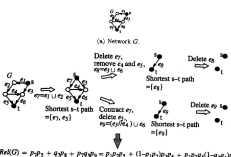
An example of how P P R and C P R algorithms perform is illustrated in Figure 2. Given a network (Figure 2a), based on the P P R algorithm (Figure 2b), according to reduction rule r5, serial links el and e2 can be first reduced to e7 with success probability PT, where P7 = PIP2.

Then, after the shortest-path-based partition and factoring, Rel(G) is decomposed as Rel(G) = q7 x R e l ( G - eT) +PTq5 x Rel(G* e7 - es) +PTP5. In the case of CPR, the network is first simplified reducing serial links el and e2 to eT. After the source-cut-based partition and factoring, Rel(G)

Terminal-Pair Reliability 361

a. Source b. Sink

r l . Links entering the source or exiting from the sink are valueless.

a. % L C )

b. O ~ O

r2. Nodes (except source and sink) with no output links or input links are valueless.

a. % ~ j ~ S i n k

b. Q . _ . l . ~ ,

'~Source

r3. Links antiparallel to node's single input link or output link are valueless.

"~'-... GL.~--_..- --'~

ReI(G1) = p, x ReI(G2)

~ . - -

~

. . . I

_{Rel(GO = Pe x Rel(G2)}

=:g:::>

(

r4. A single link going out of the source or into the sink could be contracted.

Pk = Pi x pj r5. Series link reduction.

Pk = 1-- qi × qi

r6. Parallel link reduction. Figure 1. Existing reduction rules.

is d e c o m p o s e d as R e l ( G ) = P7 x R e l ( G * eT) +

q7P3

× R e l ( G - e7 * e3). I n b o t h case, all n e w l y g e n e r a t e d s u b p r o b l e m s a r e c o n t i n u o u s l y p r o c e s s e d until s a n d t are c o n t r a c t e d o r d i s c o n n e c t e d .

3. T R I A N G L E

R E D U C T I O N

A X I O M

T h e t r i a n g l e r e d u c t i o n a x i o m [9] is a p p l i e d t o a

source-based triangle subgraph

of a g r a p h r e p r e s e n t i n g t h e n e t w o r k u n d e r c o n s i d e r a t i o n . A s u b g r a p h is defined as a s o u r c e - b a s e d t r i a n g l e s u b g r a p h if it c o n t a i n s t h e s o u r c e a n d two o n e - w a y or t w o - w a y c o n n e c t e d n o d e s t o w h i c h t h e s o u r c e is o n l y a d j a c e n t , f o r m i n g a t r i a n g l e , as shown in F i g u r e 3a. N o t i c e t h a t t h e n o t i o n o f t h e t r i a n g l e s u b g r a p h c a n b e s i m i l a r l y a p p l i e d t o a s u b g r a p h i n c l u d i n g t h e s i n k i n s t e a d ( s i n k - b a s e d ) , as s h o w n in F i g u r e 3b. F o r simplicity, w i t h o u t f u r t h e r d e c l a r a t i o n , t h e t r i a n g l e s u b g r a p h r e f e r r e d t h r o u g h o u t t h e r e s t o f t h e p a p e r is s o u r c e - b a s e d . N o t i c e t h a t t h e c o n c e p t o f t h e t r i a n g l e r e d u c t i o n c a n n o t b e a p p l i e d t o t h e cases in which t h e source (sink) is i n c i d e n t w i t h m o r e t h a n two o u t g o i n g ( i n c o m i n g ) edges d u e t o e x p o n e n t i a l l y i n c r e a s e d c o m p l e x i t y .

I n F i g u r e 3a, t h e two n o d e s t o which t h e s o u r c e is a d j a c e n t a r e d e n o t e d as n l a n d n2. T h e two links c o n n e c t i n g f r o m s to n l a n d n2, referred to as t h e

sides

of t h e t r i a n g l e , a r e l a b e l e d as esl

362 S.J. Hsu AND M. C. YUANG

(a) Network G.

Delete eT, ~ o Delete e8 sO

remove e4 and e5, ~,-o ~ • t

es=e3 U e6 t

={es}

eT=el u e2 esXl.fe6

- ~ t ~ . . ~ . Delete e9 s •

Shortest s-t path Contract e7,

={eT, es} delete es,, ~'~'t • t

eg=(e311e4 ) u e6 Shortest s-t path ={eg} ReI(G) = PTP5 + qTP8 + PTqsP9 = PlP2P5 + (1-PlP2)P3P6 + PlP2qs(1--q3q4)p6 (b) The PPR algorithm.

eGs•,•

e~s _e C ~ c t e5 • s = t Contract eT, e s S ~ s_ e l O ~ l e 4 7 e 6 = t

={e5, elo} e5,

ez=el u ez es"~te6 contract e]o S urce cut

sm ={e6}

Source cut Delete eT,

={e7, e3} contract e3, ~ ' t ~ • s = t

remove e4 and e5 Source cut ConWact e6

~

{e6}

Rel(G) = PT(P5 + q~loP6) + qTP3P6 =PlP2(P5 + qs(1--q3q4)P6) + (1-plp2)p3p 6

(c) The CPR algorithm. Legend:

* Pi(qi): the success (failure) probability of link ei.

• "U': the operation of combining series links.

• Pj =P~Pt, if ej = ek Uet.

• "//": the operation of combining parallel links.

• P1 = 1 - qkqt, ifej = ek//el.

Figure 2. PPR and CPP, algorithms--an example.

and es2 with success probabilities P81 and Ps2, respectively. The link connecting nl (n2) to n2 (nl), referred to as the base of the triangle, is labeled as ebl(eb2) with success probability Pbl(Pb2).

Notice that, if nl and n2 axe two-way connected, the base of the triangle is comprised of two links. As a result, the three nodes (s, n l , and n2), the sides (es1 and e82), and the base (ebl

a n d / o r eb2), constitute a triangle subgraph, denoted as G~.

Basically, the triangle reduction axiom transforms a graph containing a triangle subgraph to a simpler graph with the base of the triangle deleted. In the following, the axiom for the two- link base is formally stated and proved. In the case of the one-link base, similar results can be obtained by replacing Phi or Pb2 with zero.

T r i a n g l e R e d u c t i o n A x i o m

In a given graph G, as shown in Figure 4, if there exists a triangle subgraph with three nodes (s, n l , and n2), two sides (esl and es2), and the base (ebl and/or eb2), G can be transformed

Terminal-Pair Reliability 363 G

f~6, e,,W,,/p¢~'

~,

(a) A source-based triangle subgraph. Legend:

• el(p~): link l with success probability P/" • Gt: the triangle subgraph of graph G.

• G r : graph G - Gt.

• s: the source node.

• t: the sink node.

Legend:

G

¢'1

k \ Or eb2(P ebl

\

J

(b) A sink-based triangle subgraph.

Figure 3. Triangle subgraphs.

G

Gx

X

• et(pl): link l with success probability Pl. • Gt: the triangle subgraph of graph G. • Gr: graph G - Gt.

Figure 4. Triangle reduction axiom.

to G N with the base removed. The new probability Pl of link es,nl of G x connecting s to nl, and probability P2 of link es,n2 of G x connecting s to n2, are reassigned as

qslPs2Pb2 + Pslqs2Pbl + PslPs2 Pl ~- (1) qslPs2qb2 + qslPs2Pb2 + Pslqs2Pbl + PslPs2 and qslPs2Pb2 + Pslqs2Pbl + PslPs2 P2 = Pslqs2qbl + qslPs2Pb2 + Pslqs2Pbl + PslPs2" (2) Moreover, the terminal-pair reliability of the transformed graph G x , R e l ( G x ) , becomes the product of Rel(G) and the reduction factor, F

Rel ( G x ) = Rel(G) × F, (3)

where

qslPs2Pb2-{-P..lqs2Phl'4-P~lPs2

F = (Pslqs2qbl+qslPs2Pb2+Pslqs2PblWPslPs2)(qslPs2qb2+q~lPs2Pb2"+'Pslqs2Pbl+PslPs2)"

(4)

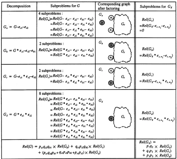
PROOF. According to the factoring theorem, Rel(G) can be partitioned to 16 subproblems, as given in Figure 5, corresponding to four graphs, Ga, Gb, Gc, and Gd. In the figure, for example, graph Gb is related to graph G by the presence of link esl and the absence of links es2 and ebl. Namely, Gb = G * esl - e s 2 - ebl. According to reduction rules r4(a) and r l , s is contracted to nl, and valueless link eb2 is removed, resulting in two equal-valued subproblems, Rel(Gb) = Rel(G * esl - es2 - ebl -- eb2) = Rel(G* e~l - es2 - ebl * eb2). As a result, G x can be associated with Gb by the presence of link e,,nl and the absence of link e,,,~, and thus, Rel(Gb) = Rel(Gx * e~,,~ 1 -e~,,~).

364 S.J. Hsu AND M. C. YUANG Decomposition G,, = G-..est-ea G b = G * esl-es2-ebl G¢ ~" G'~sl * en-eb~ G d = G*esl*es2 Subproblems for G 4 subproblems :

Rel(G,)=Rel(G- e,t- e a - ebl- ebb) =Rel(G- e , : e a - ebl * ebz) =Rel(G- e,i- e,2 * ebl- eb2) =Rel(G- e,l- e,2 * ebi * e~,2)

2 subproblems :

R e l ( G t , ) = R e l ( G * e,t- e a - eb,- eh2)

= R e l ( G * e , t - e a - et, i * eb2)

2 subproblems :

ReI(G,)=ReI(G- e,l * e a - e#l- eb2) =Rel(G- e,j * e,2 * ehj- ebb)

8 subproblems :

Rel(Ga)= ReI(G * e,I- ea * e b r ebb) = ReI(G * e~l- ea * ebl * eb2)

= R e l ( G - e,t * e , 2 - ebl * eb2) = ReI(G- e,l * e,2 * et, i * et,2) = Rel(G * e,l * ejr- ebL-- eb2)

= R e I ( G * e,, * e , 2 - ebl * eb2) = R e l ( G * e,i * e a * e b t - eb:)

=Rel(G * e~t * e,2 * e#t * e~z)

Corresponding graph after factoring

0 ( ~ G r ~

Vd

ReI(G) = P,lq,2qb' X Rel(Gb) + q,tP,2qb2 X ReI(G¢) + (P:tq,aPbl + q.,P,2Pb2 +p,@,~) X ReI(Ga) Subproblems for Gx ReI(G,) =Rel(Gr--e~.,,ce,.,, 2) =0 Rel(Gb) =Rel(Gx * e,.,,(-e,.,, 2) Rel(G~) =Rel(Gr--e,.,, i * e,.,?) Rel( G #)

=Rel(Gx * e~.~ 1 * e,,, 2)

Rel(Gx) =

Plq2 X Rel(Gb) + qlP2 × ReI(G~) + PlP2 X ReI(G#)

Figure 5. Association of l=tel(G) and Rel(Gx).

Applying t h e same logic of relating other graphs (Ga, G c , and Gu) to G x , we a t t a i n Rel ( G x ) = Plq2 × Rel ( G x * es,nl - es,n2) + qlP2 x Rel ( G x - es,na * es,n2) + PiP2

x Rel ( G x * e s , m * es,n2) (5)

= Plq2 x Rel(Gb) + qlp2 x Rel(Gc) + p i P 2 x Rel(Gd). In addition, notice t h a t Rel(G) can be expressed as

Rel(G) = Pslqs2qbl x Rel(Gb) + qslPs2qb2 x Rel(Gc)

(6)

+ (Pslqs2Pbl + qslPs2Pb2 + PslPs2) x Rel(Gd). Dividing e q u a t i o n (5) by a reduction factor F , we obtain

1 Plq2 qlP2 PiP2

x Rel ( G x ) = ---if-- x Rel(Gb) + - - ~ x Rel(Gc) + T x Rel(Gd). (7) E q u a t i n g equations (6) and (7), we a t t a i n

Rel ( G x ) = ReI(G) x F (8)

and

p l q 2 qlp2

F = Pslqs2qbl, F = qslPs2qb2, and PlP.._.._~2 F = Pslqs2Pbl + qslPs2Pb2 + P s l P s 2 . (9) R e a r r a n g i n g equation (9), we directly derive equations (1), (2), and (4) and thus, prove the

Terminal-Pair Reliability 365 T h e c o m p u t a t i o n a l complexity of triangle reduction rests on the examination of the existence of triangle subgraphs and the transformation. Clearly, examining the existence of triangle sub- graphs, namely an output-degree of the source of two and the adjacency of the source with two one-way or two-way connected nodes, only requires computational complexity of a constant time. W i t h the closed formulas given in equations (1)-(4), the computational complexity of the t r a n s f o r m a t i o n is apparent O(1).

4. R E D U C T I O N

E F F I C I E N C Y

A N A L Y S I S

F O R S I M P L I F I E D G R I D N E T W O R K

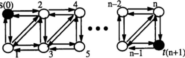
To exhibit the effectiveness of triangle reduction, we analyze the numbers of subproblems generated by P P R and C P R , with and without the triangle reduction axiom, for a s i m p l i f i e d g r i d n e t w o r k . A network with n + 2 nodes including s and t (numbered from 0 to n + 1) is defined as an n-level simplified grid network, denoted by S G n , if any three consecutive nodes of the network form a complete graph, as shown in Figure 6. For ease of description, the partition basis in P P R or C P R is selected in an increasing node number manner. The number of subproblems generated by P P R (CPR) for S G n is denoted as NSPn ( N S C ) . In S G ~ , the link incident from i to j is denoted as ei,j. In addition, the P P R and C P R algorithms with triangle reduction applied are denoted as P P R + and C P R +, respectively.

..n

n

Figure 6. An n-level simplified grid network--SGn.

LEMMA 1.

= i? / + ig / ' for n _> 2 and N S P = 1.

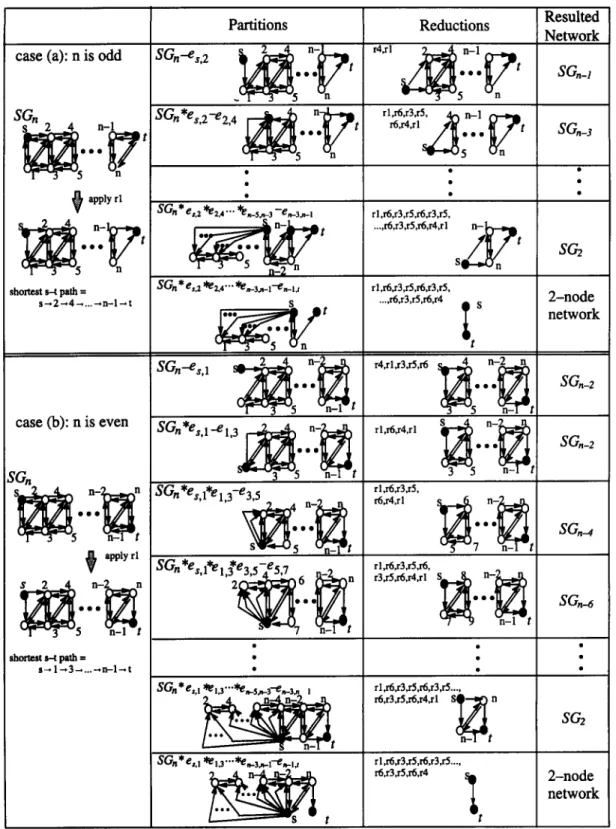
PROOF. According to reduction rules r l , r5, and r6, the fact t h a t T R of S G 1 can be directly c o m p u t e d without any partition leads to N S P = 1, for n = 1. T h r o u g h simple derivation, one can simply get t h a t N S P = 3 and N S P = 5. For n >_ 4, the derivation can be discussed in the following two cases, as illustrated in Figure 7.

CASE (a). n IS ODD. According to reduction rule r l , valueless links el,~, e2,s, e t , n - 1 , and Ct,n can be i m m e d i a t e l y removed, leading to a new shortest s - t p a t h of S G n , s ~ 2 --* 4 --* • • • --* n - 1

---* t. Based on the path-based partition and factoring, Rel(SGn) is decomposed to ( ( n - 1)/2 + 1) newly generated subproblems, namely R e l ( S G n - es,2), Rel(SGn * e8,2 - e2,4), • • •, Rel(SG~ * e~,2 * e2,4 * " " * e n - 5 , n - 3 -- en-3,n-1), and R e I ( S G n * es,2 * e2,4 * " " * e n - 3 , n - 1 -- e n - l , t ) . According to reduction rules r l , r 3 to r6, the first (n - 1)/2 subproblems can be reduced to lower-level simplified grid networks, as shown in Case (a) of Figure 7. T h e last subproblem ( S G n * es,2 *

e2,4 * ' ' " * e n - 3 , n - 1 -- e n - l , t ) can be repeatedly reduced to the simplest network with only source and sink, resulting in the generation of one subproblem. Accordingly,

= 1 + lvSL +, + 1

(lO)

366 S.J. Hsu AND M. C. YUANG

case (a): n is odd

SG~

s - 2 4 n-1 t ~ apply rl shortest s--t path = s~2~4 . . . n-l~t case (b): n is even

sG.

o • • t ~ apply rl • • n - ~ t shortest s--t path = s ~ l ~ 3 . . . n-l~t Partitions l S Gn--e s, 2 Reductions . - v ~ - 5 - n R e s u l t e d Network

SGn_I

s a n * e s 2 - . e 2 4 ~

_{• ,}

5

n) n ~ rl,r6,r3,rS, 4r~n_l _{r6,r4,rl ~ . . .} ~ n _{t SGn-3} o o . t s ~ 5 • o s • • • • @ • r I ,r6,r3,r5,r6,r3,rS, .... r6,r3,rS~6,r4,rl

SGn*

e,,2 ~e2,4 "'" ~n-5~)-3 -en-3~-i t & n - • -, -, ---_ -n SGn * e,.2 ~.4"'" *e~-3~-l-e~-l., s

SGn--.e s, 1

t

SG *e,.1-e 1,3

S G n * e s, l*e l , 3 - e 3 , 5 _ n_~ - SGn*es'l*el'~e3'5-~es'72~!O ~n~_ - n

SGn* e$, I ~ 1,3"°°I~_J~_3"~

rl,r6,r3,r5,r6,r3,r5, .... r6,r3,rS,r6,r4

t, s

r4,r 1,r3,rS,r6 ~ 5 ' n-2 n • " n - ~ t rl,r6,r4,rl ~ 5 * ' ' n - n - ~ rl,r6,r3,r5, r6,r4,rl o o o rl,r6,r3,r5,r6, r3,r5,r6,r4,rl S ~ . @o rl,r6,r3,r5,r6,r3,r5 .... r6dr3,r5,r6,r4,r 1 S n _ ~ f r 1,r6,r3,rS,r6,r3,r5 .... r6,r3,rS,r6,r4 ~ t ~3,n I

SGtI*

e$o I ~el,3... ~ce n..3,a..l"~ a.. i, t

SG2

2-node network SGn-2 SG~_2

SO~_4

SG~_~

SG2

2-node network

Figure 7. PPR. algorithm for an n-level simplified grid network.

CASE (b). n IS EVEN. According to reduction rule r l , valueless links el,s, e2,s, et,n-1, and et,,~ can also be removed, leading to a shortest s - t path of SGn, s --+ 1 --* 3 . . . . --* n - 1 --* t.

Based on the path-based partition and factoring, R e l ( S G , ) is decomposed to (n/2 + 1) newly generated subproblems, namely Rel( SGn - e8,1), Rel( SGn * e8,1 - el,3), • • •, Rel( SGn * es,1 * el,3 * • " "*e,,-s,n-3-en-3,n-1), and R e l ( S G n * e s , l * e l , 3 * ' " * e n - 3 . n - 1 - e , - 1 , t ) . According to reduction rules r l , and r 3 to r6, the first n / 2 subproblems can be reduced to SGn-2, S G , - 2 , S G n - 4 , . •.,

Terminal-Pair Reliability 367

• " * en-3,n-1 - en-l,t) can be repeatedly reduced to the simplest network with only source and sink, resulting in the generation of one subproblem. Accordingly,

= 1 + N s L 2 + NSn_2k + 1 P

k = l

(11)

= N s P _ I + NSff_2, for n > 4. From equations (10) and (11), we obtain the recurrence relation

N S P = N S P _ I + N S P _ 2 , for n > 4.

(12)

Solving equation (12), the lemma can be directly proved.

LEMMA 2.

N S C = ( 5 + - 5 - ~ ) ( l + - 2 - ~ ) n q - ( 5 - - 5 - v ~ ) ( 1 - - - 2 - ~ ) n - 1 , _{for n_> 1.}

PROOF. T h r o u g h simple derivation, one can get N S C = 1 and N S C = 3. For n > 2, according to reduction rule r l , valueless links el,s, e2,s, et,n-1, and et,n are removed, as shown in Figure 8. Based on the source-cut-based partition and factoring, Rel(SGn) is further decomposed to two new subproblems, Rel(SGn * es, 1) and R e l ( S G n - es, 1 * es,2). The former can be reduced to SGn_ 1, and the latter can be reduced to SGn-2. Thus, we obtain

N S c = N s C _ I + NsC_2 + 1, for n > 2. (13) Solving the equation, the lemma is directly proved.

sv.

O 0 0 ~ I t

l;ooq

t Resulted Partitions Reductions Network rl,r6 S G n *g $,l 2 ' n - n . o . t rl,r3,rS~-6 O Q e 5 t

" 3~5

T M

-n-I - t

SG.-I SG,,-z

Figure 8. C P R algorithm for an n-level simplified grid uetwork.

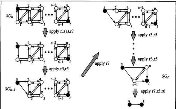
LEMMA 3. With triangle reduction augmented, both P P R + and C P R + result in the generation of only one subproblem for SGn.

PROOF. According to reduction rule r l ( a ) and triangle reduction, links el,8, e2,s, el,2, and e2,1, are first removed, as shown in Figure 9. Through reduction and contraction, SGn is further reduced to S G n - 1 , . . . , SG2, and ultimately to the simplest network with only source and sink. ] THEOREM 4. The reduction e~cieney ratios of P P R to P P R + and CPR to C P R + are O(((1 + v ~ ) / 2 ) ~ ) , for S G , , n > 2.

PROOF. Based on Lemmas 1 and 3, the reduction efficiency ratio of P P R to P P R + is N S P to one, for all n > 2. The reduction efficiency ratio of C P R to C P R +, by Lemmas 2 and 3, is N S C

368 S . J . H s u AND M. C. YUANG

~ apply rl(a),r7

~ : • : -

n - ~ t

~ apply r3,r5

SGn-1

ply r7

~ apply r3,r5

apply r3,r5

n

SC,2

n - I t

apply r7,r5,r6

~----~O t

Figure 9. T h e reduction procedures of P P R + and C P R + for an n-level triangle network.

(9) [3,6]

(13)[3,6]

(17)[3,6]

~

t

(2)[3,6]

,6,,3:6~. t

(10) [3,6]

(14)[3,61

(22)[6,11]

~

t

( 3 ) [ 3 ' 6 ] s ~ t

(7) [3,61

s ~ t

(15)~

(19)[6,12]

(23)

[61

_s

(8)[3,6]

s ~ ~ ) D t

(12)[3,6,14]

(16)[.', ,6]

(20)[6,13] (24)[6,111

A complete net-

work

with 10 nodes

Figure 10. Benchmarks.

T e r m i n a l - P a i r R e l i a b i l i t y 369

to one, for all n >_ 1. Thus, we attain

= O - , for n > 2.

5 . P E R F O R M A N C E C O M P A R I S O N S

- 1 ( 1 4 )

To demonstrate the effectiveness of triangle reduction, we experimented on various networks using four algorithms, PPR, CPR, P P R +, and CPR +, which were implemented in C language and executed on Sun ServexStation 5. The experimented networks include the benchmarks [3,6,7,11- 14], as summarized in Figure 10, and randomly generated networks with various link degrees. In all experiments, two performance metrics, the number of subproblems and computation time, have been observed.

Figures 11 and 12 show performance comparisons among these four algorithms under published benchmarks. In Figure 11, as was expected, the number of subproblems generated by either the P P R + or the C P R + algorithm is lower than that of both the P P R and CPR algorithms for all benchmarks. The performance superiority is particularly prominent under Benchmarks 1, 3, and 22, owing to the existence of higher numbers of triangle subgraphs. As for computation time, P P R + (CPR +) also outperforms P P R (CPR) algorithm in all (most of the) benchmarks, as shown in Figure 12.

8. 18

6 6 4 4 2 2 0 0 (1) 25 20 15 10 5 (5) 0 15 12 9 6 3 (9) 0 40 32 ~ 30 24 20 l e ! n . L~ P ~ CPRp~ + CPR + k l ~ PPR CPRPPR + ~ R + ' 0 0 , I x l O ~ ' 16

i

L, oo ~ 9 o o ~ l ~1 30 24

,°o8

4 2 0 300 250 200 150 PPR CPR PPR + CPR + PPR CPR PPR + CPR + PPR CPR PPR + CPR + PPR CPR PPR + CPR + F i g u r e 11. C o m p a r i s o n s o f t h e n u m b e r o f s u b p r o b l e m s u n d e r b e n c h m a r k s .

370 S . J . H s u AND M. C. YUANG

o.e ~ o.s ~ ~ o.~ ~

tl

2.s ~ I

o.4 ~ o.4 ~ 0.~ ~ - ~ - ~ w m u ~ l 2.,, ~ ~ o.z ~ 0.~ ~ 0.~ ~ I 2.2 • O ~ 0 ~ = - ~ - = ~ - ~ - ~ 0 ~ " I 2 '< .. . . " ' " 2 PPR CPR PPR +CPR + 3 - PPR CPR PPR + CPR + 4 PPR CPR PPR + CPR + 0 O l ( 9 3 PPR CPR PPR + C P R + 1 PPR CPR PPR + CPR + 17- PPR CPR PPR + CPR + 12 PPR CPR PPR + CPR + 50 4 0 0 2 40 ~ 300 0 30 1 ~ ~ PPR CPR PPR + CPR + 1 PPR CPR PPR + CPR +

, , . ~ ~ ] .

..

rn,~

t

I

, 8 o

~ ~ ~ + + 1

a

50 lzo

~

t

1

1~]~ 120 7 40 80

~

CPR + 2 100 ~ l ( 2 ~ 2 ~ PPR CPRPPR+ CPR + F i g u r e 12. C o m p a r i s o n s of c o m p u t a t i o n t i m e u n d e r b e n c h m a r k s .

Normalized number of subpmblems 30 + - - - + PPR 25" -': PPR + "¢ 20- Jl II 15- I I I I ~ 1 \

,J\.,

I ' , , . ~ / ~I L ÷ O 7 T T T T T . T T T T T T T T T T T T T T T T 7 1 5 10 15 20 24 Benchmark (a) C o m p a r i s o n s b e t w e e n P P R a n d P P R +.

Normalized number of subproblems

30, ___ 25 20 15 10 !+---+ CPR • • CPR + II II I I l \ I I O, 7 7 7 7 7 7 7 7 7 7 7 7 7 7 7 7 7 7 7 7 7 7 7 7 1 5 10 15 20 24 Benchmark (b) C o m p a r i s o n s b e t w e e n C P R a n d C P R +. F i g u r e 13. C o m p a r i s o n s of t h e n u m b e r of s u b p r o b l e m s u n d e r b e n c h m a r k s .

Normalized computation time 4.5" ÷ - - - ÷ PPR ¢ "- P P R + A 2.5- ~ A , I I / I I I 1.5- \ / \ ,'~ '~'¢ i 2 ÷ 0.5 5 10 15 20 24 Benchmark

Normalized computation time 4.5~ . . . I÷---+ CPR 3.5 ~ 7 * * CPR+ i

2.,i

,!

,,/\,

1 5 10 15 20 24 Benchmark (a) C o m p a r i s o n s b e t w e e n P P R a n d P P R +. (b) C o m p a r i s o n s b e t w e e n C P R a n d C P R +. F i g u r e 14. C o m p a r i s o n s of c o m p u t a t i o n t i m e u n d e r b e n c h m a r k s .

T e r m i n a l - P a i r Reliability 371 Normalized number of s u b p m b l e m s 3.0- + _ _ _ + P P R ,___ ._._, p p R + 2.5- ~. ~ - t ----r'''+ / ~v 2.0- _/ ,r

/

1.5- / +~ ] , 0 " ; ~. - ~ * . - - - - q D - - ~ O - - - , l ~ - - m • 0.5 . . . 1 2 3 4 5 6 7 8Lin~ 10 degree (a) C o m p a r i s o n s b e t w e e n P P R a n d P P R +.

Normalized number of subproblems 3.0- ÷ - - - + C P R 2.5" ~---" ~ CPR+ 2.0- 1.5- 1.0" s , - - - , - - ~ - - - ~ - - o - - - t - - - ¢ - - • , 0.5 . . . . 10 1 2 3 4 5 6 7 ~Lin~degree (b) C o m p a r i s o n s b e t w e e n C P R a n d C P R +. F i g u r e 15. C o m p a r i s o n s of t h e n u m b e r of s u b p r o b l e m s u n d e r r a n d o m l y g e n e r a t e d networks.

Normalized computation time 2.0 + - - - + P P R 1.8 e - - - . . - - - e p p R + i+

f

1.6 _A,.~¥ / 1.4 / . / / , k \ , ~ ~ ¥ / 1.2 / 1.0 ~ ~" ~ *-"'~ " " ~ ' * ""*- "• •

0.8

i ~ ~ ~ ~ 6 ~ s 9

]0

Link degree (a) C o m p a r i s o n s b e t w e e n P P R a n d P P R +. F i g u r e 16. C o m p a r i s o n s of c o m p u t a t i o n t i m e

Normalized computation time 2.0] + - - _ _ + C P R 1.8] e----. - - 4 CPR + 1.6] 1.4~ I l "2 t -~-~ 1 . 0 ~ : - - - * - - 4 . - - - e - - - ~ - ~ B - ~ e - - - m m 0.8L . . . . 1 2 3 4 5 6 7 8 9 10 Link d e g r e e (b) C o m p a r i s o n s b e t w e e n C P R a n d C P R +. u n d e r r a n d o m l y g e n e r a t e d networks• Normalized a m b e r of subproblems 1.2 1.0" ¢~ ; - ~ 4 - - - - ~ - -*---- • ----e- - * • \ 0.8- _{\ \} \ 0.6 _\ \ x ~ 4." "6" -....-4"- ,me. 0.4 + - - - * - - - r +__~ + p p R + • - - - . - - 4 CPR + 0 . 2 , , , , , J , , , i i , 1 2 3 4 5 6 , (a) C o m p a r i s o n s b e t w e e n P P R a n d P P R +.

Normalized computation time

11" 1 # - - - ¢ - , / / ~ " - ~ \ / N-..x i-~ 0.84 0.64 0.4H I + - - - + PPR + I t . - - . ---* C P R + 0.2L . . . . , o 1 2 3 4 5 15 7 i d e g r e e (b) C o m p a r i s o n s b e t w e e n C P R a n d C P R +. F i g u r e 17. P e r f o r m a n c e c o m p a r i s o n s u n d e r r a n d o m l y g e n e r a t e d networks.

Figures 13 and 14 show the performance improvement of P P R + / C P R + compared to P P R / C P R , under all benchmarks. In Figure 13a, the number of subproblems generated by P P R + is improved by a magnitude of four. As shown in Figure 13b, while the improvement ratio of C P R + to C P R is less significant than that of P P R + to PPR, C P R + still outperforms C P R by a magnitude of two. In Figure 14, we have observed that the contribution of the triangle reduction to the computation time is more significant in P P R + than in C P R + as well.

Figures 15 and 16 display the performance improvement of P P R + and C P R + under a set of randomly generated networks, from sparse to dense, with 15 nodes in each network. As shown in both figures, the improvement of P P R + in both performance metrics increases with the link degree of the network. In contrast, the improvement of C P R + is almost irrelevant to the link degree. By drawing direct comparisons between P P R + and C P R + in Figure 17, we have learned that, while P P R yields poorer performance [6] than CPR, P P R + with triangle reduction augmented achieves surprisingly better performance under sparse networks• As for denser networks, C P R + still outperforms P P R + due to its simplicity in determining the partition basis [6].

372 S.J. Hsu AND M. C. YUANG

6. C O N C L U S I O N S

This paper proposed a triangle reduction which transforms a graph containing a triangle sub- graph to t h a t excluding the base of the triangle, with constant complexity. The paper also proved t h a t both the reduction efficiency ratios of P P R to P P R + (i.e., N S P to one) and C P R to C P R + (i.e., N S C to one) are O(((1 + v/5)/2)u), for simplified grid networks. The paper further provided an assessment of the effectiveness of triangle reduction on partition-based T R algorithms with respect to the number of subproblems and computation time through published benchmarks and randomly generated networks. Experimental results revealed that, P P R + and C P R + outperform P P R and C P R algorithms under most of the benchmarks and randomly generated networks. The improvement of P P R + in both performance metrics increases with the link degree of the network, while the improvement of C P R + is almost irrelevant to the link degree. In addition, even though P P R was shown in literature to exhibit much poorer performance than CPR, P P R + achieves surprisingly better performance under sparse networks.

R E F E R E N C E S

1. S. Rai, A. Kumar and E.V. Prasad, Computer terminal reliability of computer network, Reliability Engineer- ing 16, 109-119, (1986).

2. S. Rai and A. Kumar, Recursive technique for computing system reliability, I E E E Trans. Reliability 1:t-36, 38-44, (April 1987).

3. S. Soh and S. Rai, CAREL: Computer aided reliability evaluator for distributed computing networks, I E E E Trans. Parallel ~4 Distributed Systems 2, 199-213, (April 1991).

4. V.A. Netes and B.P. Filin, Consideration of node failures in network-reliability calculation, I E E E Trans. Reliability R.-45, 127-128, (March 1996).

5. W. Ke and S. Wang, Reliability evaluation for distributed comPuting networks with imperfect nodes, I E E E Trans. Reliability R-46, 342-349, (Sep. 1997).

6. Y.G. Chen and M.C. Yuang, A cut-based method for terminal-pair reliability, I E E E Trans. Reliability 1:t-45 (3), 413-416, (September 1996).

7. N. Deo and M. Medidi, Parallel algorithm for terminal-pair reliability, I E E E Trans. Reliability R-41, 201- 209, (June 1992).

8. S. Hariri and C.S. Raghavendra, SYREL: A symbolic reliability algorithm based on path and cutset methods, I E E E Trans. Computers C-36, 1224-1232, (Oct. 1987).

9. S.J. Hsu and M.C. Yuang, Efficient computation of terminal-pair reliability using triangle reduction in network management, In Proc. ICC, pp. $8.5.1-$8.5.5, (1998).

10. M. Macgregor, W.D. Grover and U.M. Maydell, Connectability: A performance metric for reconfigurable transport networks, I E E E J. Select. Areas Commun. 11, 1461-1469, (Dec. 1993).

11. L.B. Page and J.E. Perry, Reliability of directed networks using the factoring theorem, I E E E Trans. Reliability R-38, 556-562, (Dec. 1989).

12. D. Torrieri, An efficient algorithm for the calculation of node-pair reliability, Proc. I E E E M I L C O M 91, 187-192, (Nov. 1991).

13. D. Torrieri, Calculation of node-pair reliability in large networks with unreliable nodes, I E E E Trans. Relia- bility R-43, 375-377, (Sept. 1994).

14. Y.B. Yoo and N. Deo, A comparison of algorithms for terminal-pair reliability, I E E E Trans. Reliability R-37, 210-215, (June 1988).