AN EFFICIENT METHOD FOR UNCONSTRAINED OPTIMIZATION PROBLEMS OF NONLINEAR LARGE MESH-INTERCONNECTED SYSTEMS

IEEE TRANSACTIONS ON AUTOMATIC CONTROL, VOL. 40, NO. 3, MARCH 1995

T. J. Su and C. G. Huang, "Robust stability of delay dependence for linear uncertain systems," IEEE Trans. Automat. Contr., vol. 37, pp. 1656-1659, 1992.

J. N. Franklin, Matrix Theory. Englewood Cliffs, NJ: F'rentice-Hall, 1968.

R. K. Yedavalli and 2. Liang, "Reduced conservatism in stability robustness bounds by state transformation," IEEE Trans. Automat. Contr., vol. AC-31, pp. 863-866, 1986.

An Efficient Method for Unconstrained

Optimization Problems of Nonlinear

Large Mesh-Interconnected Systems

Shin-Yeu Lin and Ch'i-Hsin Lin

Abstmet-We present a new efficient method for solving unconstrained optimization problems for nonlinear large mesh-interconnected systems. This method combines an approximate scaled gradient method with a black GaussSeidel with line search method which is used to obtain an approximate solution of the unconstrained quadratic programming subproblem. We prove that our method is globally convergent and demon- strate by several numerical examples its superior efficiency compared to a sparse matrix technique based method. In an example of a system of more than 200 variables, we observe that our method is 3.45 times faster than the sparse matrix technique based Newton-like method and about 50 times faster than the Newton-like method without the sparse matrix technique.

I. INTRODUCTION

In this paper we consider the following unconstrained optimization problem for a nonlinear large mesh-interconnected system

min J ( x )

zEPn

where the objective function J:

R"

--+

R

is continuously differen-

tiable, bounded from below and satisfies the Lipschitz condition that there exists a constant Ii

>

0 such that I1VJ(sl) - VJ(x2)112

5

Iillzl - x z ~ ~ z , Vs1, xz E SR". A general descent algorithm, which is called a scaled gradient method in [ l ] , for solving problem (1) uses the following iterations

where k denotes the iteration index, T~ is a step-size, and sk is the solution of

(3) in which C'(J?) is a positive definite matrix.

For a large mesh-interconnected system, if C ( x k ) is selected so that (2) is a Newton or Newton-like method, C ( x k ) may be a sparse matrix. The solution of (3), which is the solution of the linear system

(4)

can be obtained using the sparse matrix technique, which is a very powerful means for solving linear equations in a circuit system [2] or

Manuscript received October 19, 1993; revised March 8, 1994. This research work is supported by National Science Council in R.O.C. under Grants NSC-82-0404-E-009-166 and NSC-79-0404-E-009-48.

The authors are with the Department of Control Engineering, National Chiao Tung University, Hsinchu, Taiwan.

IEEE Log Number 9407217.

an electric power system [3]. This technique effectively reduces the amount of computer memory needed and improves the computation time dramatically because it stores only nonzero elements and ignores operations involving zeros in the solution process [2]. Thus, a sparse matrix technique based Newton or Newton-like method is much more efficient than a method with quadratic convergence rate.

In this paper, we will present a new method for solving (1) for a large mesh-interconnected system to compete with a sparse matrix

technique based method. Our method combines an approximate

scaled gradient method with a block Gauss-Seidel with line search (BGSLS) method. Although each of the above methods is well known, combining them into one method is a new approach. The basic idea behind this method is to preserve the advantages and discard the disadvantages of the block Gauss-Seidel method. We have observed in many numerical experiments [4] that the block Gauss-Seidel method approaches its convergence point very fast in the first few iterations and then slows down around that point. This fact indicates that the block Gauss-Seidel method is better suited for use as a descent direction generator rather than as an optimization algorithm by itself. To improve the quality of the descent direction further, we use an exact line search at the end of each cycle of the block Gauss-Seidel method and thus form a BGSLS method. Executing the BGSLS method for a finite number of iterations with appropriate stopping criteria will generate the descent direction needed for the approximate scaled gradient method. We will show in this paper that our method is a globally convergent descent algorithm. It is difficult to give an analytical convergence rate for our method because of the nature of the method. However, since the major computation required by our method lies in the execution of the BGSLS method, our method will be efficient if the BGSLS method can generate an effective descent direction in several iterations. Intuitively, our method should be efficient and effective, for two reasons: i) only small minimization problems are involved in each iteration of the BGSLS method and ii) the exact line search used at the end of each iteration of the BGSLS method greatly improves the quality of the descent direction.

11. SOLUTION METHOD

A . The Approximate Scaled Gradient Method

The approximate scaled gradient method [ 11 is

where i k is an approximate solution of (3) and 5' is a step-size. To ensure global convergence, we use Armijo-type rule to determine the step-size by

y k = $ 7 1 1 k X (6)

where 0</3<1, X>O, and mk is the smallest nonnegative integer m

that makes the following inequality hold for some positive constant I i z

Remark 2.1: a) Condition (7) is to ensure a sufficient decrement of the objective function obtained in each iteration of (5); the satisfaction of this condition serves as a terminating criteria for our Armijo-type step-size rule (6). b) As will be shown in Theorem 2.1, the matrix

$ C ( x k ) - 1 < 2 I being nonnegative definite is a sufficient condition for (5) to converge. This sufficient condition provides a value for I<*.

0018-9286/95$04.00 0 1995 IEEE

IEEE TRANSACTIONS ON AUTOMATIC CONTROL, VOL. 40, NO. 3, MARCH 1995 49 1

Lemma 2.1: Suppose (3) is solved by a descent iterative algorithm

starting from s = 0 for any arbitrary number of iterations, and let i k

denote the final value of s. Then V J ( Z ' " ) ~ ~ ~

<

0.

This lemma can easily be verified by the fact that

$ ( ? k ) T C ( z k ) i k

+

V J ( X ' ) ~ ? '

<

0. Thus, our approximate scaled gradient method (5) will be an efficient descent algorithm for solving (1) if the descent algorithm we employ to obtain ik is efficient.

B . Block Gauss-Seidel with Line Search (BGSLS) Method

I ) One Block Gauss-Seidel Cycle: Let us partition s into p sub- vectors such that s = [sls:!

. . .

s p l T . Then one block Gauss-Seidel cycle is to perform

min 8 % $ s T ~ ( r k ) s

+

VJ(Z')'s ₍₈₎

from i = 1 to p. In (8), the subvector s z is taken as the vector of minimizing variables while the variables in the subvectors SI,

. .

,

s , - I , sZ+l,

. . .

, s p are held fixed at their current values. Note that compared to (3), (8) is a small unconstrained minimization problem for every i .

Remark2.2: On the partition of the s-vector, there are two ex-

tremes corresponding to p = 1 and p = n. The case of p = 1 is not the interest of this paper. For the case of p = n, the descent direction generated by (8) has very poor quality. Thus, a good partition should take the following two factors into account: a) computational burden of solving (8) and b) the quality of descent direction generated. In fact, the above two factors have conflicting interests; at this stage, we have not yet achieved an optimal way to partition the s- vector. Nonetheless, for a network-structure like system, it would be beneficial if each partitioned subnetwork is mesh-interconnected, and the sizes of all subnetworks do not differ much.

2 ) Optimal Step-Size: Let s(') denote the value of s after solving (8) for s,. Then s(O) represents the initial value and the final value of s for one block Gauss-Seidel cycle. Suppose s(O) is not the optimal solution of (3). Then the following inequality holds

; ( s ( o ) ) T C ( x k ) S ( O )

+

V J ( z : " ) T s ( O )

>

+(S(P))TC("k)S(P)

+

V J ( z k ) T s ( P ) . (9) Furthermore, because C ( x k ) is positive definite, i s T C ( z k ) s

+

V J ( z k ) * s is a convex function in s. Based on this fact, we may verify that

;

( , ( P I ) C(

2 )

s(p)

+

VJ(

2)

s(p)

2

$ ( s ( 0 ) ) T C ( z k ) S ( o )

+

VJ(z"Ts(0)

+

[ C ( S k ) S ( 0 )

+

V J ( z k ) l T ( s ( P ) - S(O))}. ₍₁₀₎

Then, combining (9) and (lo), we obtain the following lemma.

Lemma 2.2: Let :

do)

and

dP)

denote the initial and final values of s-variables, respectively, for one block Gauss-Seidel cycle of the BGSLS method. Suppose

do)

is not an optimal solution of (3). Then (1 1) -

do)

is a descent direction Therefore, we can determine the exact optimal step-size & to update

[ C ( X k ) S ( O )

+

V J ( z y ( s ( P )

-

do))

<o.

The above inequality implies that of ; s T ~ ( x k ) s

+

~ ~ ( 2at )s = ~ s(O). s

the variable s by

+

( i . ( J P ) -

p))

(12)

su = s(o)

where su denotes the updated s, and the optimal step-size

ci. = - [C(.Z?)s(O)

+

VJ(.rk)]T(s(") - d o ) )

[g(P) - "(O)]TC(""[S(P) - S(O)] (13)

is obtained by solving the following one-dimensional minimization problem

min ,220 {$[s(O)

+

a(s(p)

-

s ( O ) ) ~ ~ ~ ( . r ~ ) [ s ( ~ )

+

a ( s ( p ) - s(O)

)I

+

V J ( z k ) T [ s ( O )

+

a p-

P))]},

(14) 3 ) One Iteration of the BGSLS Method: The following three op-

erations form one iteration of the BGSLS method: i) execute one block Gauss-Seidel cycle; ii) determine &; and iii) update su

.

's will be the initial value s(O) for the next iteration of the BGSLS method.

4 ) Convergence of the BGSLS Method: This iterative BGSLS

method will converge to the solution of (3), as described in the following lemma. The proof of the lemma is given in the Appendix.

Lemma 2.3: Assuming that there exists a constant IC2

>

0 such that $ C ( z k ) - K:!I is nonnegative definite for all I', then a) the BGSLS method is a descent method, and b) any limit point of the sequence generated by the BGSLS method is a solution of (3).

5 ) Stopping Criteria of the BGSLS Method: As pointed out in

Section I, the BGSLS method approaches a solution point of (3) very quickly in the first few iterations; however, it then slows down around that point. In fact, it was this characteristic of the BGSLS method that gave us the idea of combining it with the qpproximate scaled gradient method. Therefore, to obtain the i k needed in (5), we do not need to execute the BGSLS method until it converges. In fact, we can stop the BGSLS method after a finite number of iterations. Consequently, one of the stopping criteria of this method is if the improvement of the objective function satisfies

Q ( t )

-

Q ( t

+ x 100%

<

E%

(15)

Q ( t )

where Q ( t ) = $ s ( t ) T C ( z k ) s ( t )

+

o J ( ~ ~ ) ~ s ( t ) ,

t denotes the iteration index of the BGSLS method, and

E%

is a preselected percentage. To ensure that (5) converges, another stopping criteria

I l s ( t

+

1)112

<

A-1llVJ(zk)llz (16) for some h-1

>

0, for all

t

>

t', where t' is a finite positive integer,

should also be satisfied. Then, the s ( t

+

1) which satisfies stopping criteria (15) and (16) will be set as i k . An explanation of the need for (16) Till be given in the proof of Theorem 2.1. The existence of

IC1 and

t

is ensured by the following corollary, the proof of which is also given in the Appendix.

Corollary2.1: Let { s ( t ) } denote a sequence generated by the BGSLS method. Under the assumption of Lemma 2.3, there exists a t

sue!

that Ils(t)llz > KIIIVJ(zk)l12 for some l i l

>

0 and for all

t

>

f

.

C . The Algorithm for the Solution Method and its Convergence

Combining Lemma 2.1 and Lemma 2.3 then proves that our method is a descent method.

Lemma 2.4: The combination of the approximate scaled gradient

method (5) and the BGSLS method, supplemented by the stopping criteria (15) and (16), is a descent method for solving (1).

1 ) The Algorithm: We are now ready to state our algorithm as

follows: Given data: i) s = [SI, s2,

..

. , splT, ii) the values of X(>O) and

8(0

<

P

<

1) in Armijo-type rule, iii) the value of

E%(

2

0%) in (15), and iv) a positive constant l i ~ which meets the assumption in Lemma 2.3.

Step 0: Set the values

d o )

and set k = 0.

Step I : Set

t

= 1 and set s ( t ) = 0.

Step 2: Set i = 1 and s ( O ) ( f ) = s ( t ) .

Step 3: Solve (8) to obtain s('). If i = p , go to Step 5; otherwise, set i = i

+

1 and repeat this step.

-492 IEEE TRANSACTIONS ON AUTOMATIC CONTROL, VOL. 40, NO. 3, MARCH 1995

Step 4: Compute

Step 5 : Update s ( t

+

1) = s ( ' ) ( t )

+

&(t)[&"(t) - s ( O ) ( t ) ] .

Step 6: If (15) and (16) are satisfied, set

R k

= s ( t

+

1) and go to Step

7; otherwise, set

t

= f

+

1 and retum to Step 2.

Step 7: Set ni = 0.

Step 8: If J ( s k

+

/3"Agk) - J ( . r k )

5

-(1i2/2)DmAllRk[l~, set

yk = $"'Ax; otherwise, set m = m

+

1, and repeat this step.

Step 9: Update xk+' = x k + y k i k , set

k

= k

+

1, and retum to Step 1. 2 ) Convergence of the Algorithm: The following theorem ensures

the convergence of our algorithm. A proof of the theorem is given in the Appendix.

Theorem2.1: Let {sk} denote the sequence generated by our algorithm. Under the assumption of Lemma 2.3, limk-- V J ( e k )

= 0.

Remark2.3: The values of A, /3, and do not affect the convergence but will influence the efficiency of our method. Thus, these values can be determined empirically for individual systems.

3 ) Stopping Criteria of the Algorithm: From Theorem 2.1, we see

that as

k

+ 00, i k ---t

0;

however, for practical considerations, our

algorithm will stop when l R k l -

<

F for a reasonable accuracy.

( t ) - s(O) ( t ) and determine &( t ) by (13).

111. EXAMPLES

Most electric power systems are nonlinear large mesh- interconnected systems. The weighted least squares problem in power system state estimation is a typical unconstrained optimization problem and thereby is an adequate example for demonstrating the computational efficiency of our method.

A . The Weighted Least Squares Problem in Power System State Estimation

The power system state estimation problem [6] can be briefly described as follows: For an 1-bus' power system, the voltage magnitudes and phase angles of all buses constitute the states of the system. Because the bus phase angle cannot be measured, the states of the system have to be estimated based on available measurements, which are functions of the states, such as power transmission line flow, bus voltage magnitude, bus power injection, and transformer tap. All such measurements can be expressed in a general form as z = h ( x )

+

q . where x is a 21-dimensional vector of state variables, z is an m -dimensional vector of measurements, k denotes m nonlinear measurement functions which are twice continuously differentiable, and q represents an m-dimensional Gaussian random vector of measurement errors with an m x m diagonal covariance matrix R. A common formulation [5] of this state estimation problem is to solve the following weighted least squares problem'

m i n J ( s ) ( = 3. $ [ z - k ( ~ ) ] ~ R - ' [ z

-

h ( x ) ] ) .

Since h(s) is twice continuously differentiable, J ( z ) in (17)

is twice continuously differentiable and thereby satisfies Lipschitz condition. Taking n = 21, the J ( x ) meets the assumptions given in Section I.

Note: For an authentic power system state estimation [ 6 ] , bad dati processing has to be associated with the solution of (17); if bad measurements are present, they should be eliminated, and the states re-estimated. However, for the purposes of this paper, we will focus on solving (17) only.

'

The buses of the power systems considered here are similar to nodes in an electrical network.

The phase angle of the slack bus is considered to be a known value.

B. Conventional Approach

In general, the Newton method may fail to solve (17) because the Hessian matrix of (17) may not be positive definite. Thus, the conven- tional approach in the power system literature [6] uses a Newton-like method, which is ( 2 ) with C ( . r k ) = ~ H ( T ' ) ~ R - ' H ( ~ ~ ) in (3), where H ( r k ) = V k ( r k ) . However, H ( J ? ) ~ R - ' H ( X ~ ) may be singular or ill-conditioned, since it is only positive semidefinite. To cope with this difficulty, we can modify the above C ( s k ) to ensure the positive definiteness by setting C ( x k ) = 2 H ( s k ) T R - ' H ( x k )

+

61, where 6 is a small positive real constant and I is the identity matrix. We see that under this modification, the only assumption needed in Theorem 2.1, $ C ( x k ) - IC21 is nonnegative definite, is satisfied by taking

Iiz

= (6/2). Furthermore, the numerical stability of our algorithm is guaranteed if 5 is not too small. Consequently,

(4) becomes

The matrix ~ H ( T ~ ) ~ R - ' H ( T ~ )

+

S I and the matrix

H ( . z ~ ) ~ R - ' H ( . ~ ~ ) are sparse, and (18) can be solved using the sparse matrix technique.

Remark3.1: a) Because H ( T ' " ) ~ R - ~ H ( X : ' ; ) may be ill condi- tioned, methods that use an orthogonal transformation technique to solve

~ H ( X ~ ) ~ R - ' H ( L ~ ) S

= - V J ( . c k ) has been developed [7].

However, these methods are computationally very inefficient. b) In

[6], the step-size 7 k is set to be 1 for all k. In fact, with a constant step-size such as this there is no guarantee that ( 2 ) will converge. c) There are other methods in the power system literature that can obtain an approximate solution for state estimation using a decoupling approach [8]. However, these methods are beyond the scope of this paper, since we are concerned only with methods that solve (1)

exactly.

C . Application of the Proposed Method

Let us partition the power system network into p (

>

1) subnetworks such that each subnetwork is a connected graph in the topological sense. Let B, denote the set of buses of the ith subnetwork; then

S B , denotes the subvector of s corresponding to states of the ith subnetwork. Replacing s,, C ( s k ) ) , and V J ( r k ) in the proposed algorithm by S B , , ~ H ( x ~ ) ~ R - ' H ( ~ : " )

+

6 1 , and H ( s k ) R - ' ( z - h( T ~ ) ) , respectively, we can apply the proposed algorithm directly to (17). Analogous to (S), we see that S B ~ , . .

.,

S B , - ~ , S B , + ~ ,

. . .

, S B ~ are held fixed in the ith minimization problem

whose solution can be obtained by solving a small set of linear equations involving only the ith subnetwork and the boundary buses outside the ith subnetwork [ 9 ] .

D . Test Results

We applied our method, the sparse matrix technique based Newton- like method, and the Newton-like method without sparse matrix technique to the weighted least squares problem in state estimation of the IEEE 30-bus power system and the IEEE 118-bus power system. For the cases under consideration, the IEEE 30-bus system was partitioned into three subnetworks, as shown in Fig. 1, in which each subnetwork is indicated by closed dashed contours. The IEEE

118-bus system is partitioned into eight subnetworks. Because of the limitation on the length of this paper, we can not include here the figure of the IEEE 118-bus system, however, this figure can be found in [lo]. Nonetheless, we list the bus number of the buses of each subnetwork in the following. Subnetwork 1 contains buses 1 to 14,

IEEE TRANSACTIONS ON AUTOMATIC CONTROL, VOL. 40, NO. 3, MARCH 1995 493

TABLE I

COMPARISON OF OUR METHOD WITH NEWTON-LIKE METHOD WITH AND WITHOUT SPARSE MAT~IX TECHNIQUE

Final objective value Average CPU time (seconds) Speedup ratio

I I I

I J I -

NLWTS(*) NLWS(O) Our method NLWTS(*) N L W S ( ~ ) Our method I -

I I I -

System

method method method (I) method (11) @I) I I

EEE-30 bus 15.88 15.88 15.88 0.99 0.46 0.27 2.15 3.67 1.70

IEEE-I 18 bus 43.05 43.05 43.05 16.53 5.49 1.59 13.94 48.13 3.45

' - - - A I

- - -

3 I

Fig. 1. The IEEE 30-bus system and three partitioned subnetworks.

and bus 117. Subnetwork 2 contains buses 15 to 19, buses 27 to 32, and buses 113 and 114. Subnetwork 3 contains buses 20 to 26, buses 70 to 76, and bus 118. Subnetwork 4 contains buses 33 to 47. Subnetwork 5 contains buses 50 to 61, and buses 63 and 64. Subnetwork 6 contains buses 48, 49, and 62, buses 65 to 69, buses 77 to 81, and buses 97, 98, and 116. Subnetwork 7 contains buses 82 to 96. Subnetwork 8 contains buses 99 to 112. Note that each subnetwork contains about 10 to 20 buses in mesh-interconnected structure though the bus numbers are not consecutive.

In both cases, we took the real-power flow and the reactive- power flow of all transmission lines of each individual system as the measurement data and assumed that some of these are bad data. We set the parameters in our algorithm as follows:

S

= 0.01,

P

= 0.9 for both systems, <% = 50% for the IEEE 30-bus system, and

E%

= 10% for the IEEE 118-bus system, X = 1.05, 1.10, 1.15 for the IEEE 30-bus system, and X = 1.25, 1.30, 1.35 for the IEEE 118-bus system. Note that each value of X corresponds to one computer run. We used various values of X to test Armijo-type rule and average the CPU time. The accuracy E in the stopping criterion of our algorithm, which is described in Subsection 11-C-3), was set to be lo-* for both cases. We used a Sun 4/60 workstation to test our algorithm. The simulation results for the case of the IEEE 30-bus system and the case of the IEEE 118-bus system are shown in Table I. The average CPU time of our algorithm is the average CPU time of the computer runs with various values of X reported on the Sun 4/60 workstation. We also solved the same cases for both systems using (2), the sparse-matrix technique based Newton-like method, with the same setup of Armijo-type rule and same initial guess as our method on the same Sun 4/60 workstation. We used Iskloo

<

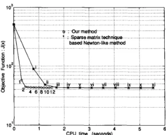
5 = lo-' as the stopping criteria for the sparse matrix technique based Newton-

like method, the test results for which are also shown in Table I. We also applied the Newton-like method without using the sparse matrix technique to the same cases on the same workstation with the same setup of Armijo-type rule, same initial guess, and same stopping criteria as the sparse matrix technique based Newton-like method. The resulting average CPU times are also reported in Table I for the cases of both systems. We see that our algorithm achieved the same final objective value as the Newton-like methods. As expected, the sparse matrix technique based Newton-like method was much faster than the Newton-like method without the sparse matrix technique in both cases, especially in the case of the IEEE 118-bus system, which has more sparsity. Compared to the sparse matrix technique based Newton-like method, our method also performs better with the larger system. From the speedup ratio shown @Table I, we see that in the case of the IEEE 118-bus system, our method is 3.45 times faster than the sparse matrix technique based Newton-like method and 48.13 times faster than the Newton-like method without the sparse matrix technique. This demonstrates the dramatic increase in efficiency provided by our method. In order to better appreciate the merits of our algorithm, in Fig. 2 we describe the details of the progression of our algorithm and the Newton-like method with the sparse matrix technique in solving the case of the IEEE 118-bus system when X = 1.35. The result of our algorithm is shown by the curve marked with circles o and associated with the Arabic numeral iteration index. Each circle indicates the CPU time accumulated (horizontal axis) at that iteration versus the corresponding value of the objective function (vertical axis) in the progression. The curve marked with asterisks

*

and associated with the Roman numeral itqation index corresponds to the Newton-like method with the sparse matrix technique. Our algorithm takes 12 iterations to meet the stopping criteria

likl,

<

lo-*, while the sparse matrix technique based Newton-like method takes only 11 iterations to meet the stopping criteria Isklm

<

lo-'. However, we see that the amount of CPU time taken up by each iteration of our algorithm is far less than that for each iteration of the Newton-like method with the sparse matrix technique. This shows the effectiveness and efficiency of using the BGSLS method to generate the descent direction. Furthermore, when our algorithm has nearly reached the optimal objective value, the Newton-like method with the sparse matrix technique has just finished its first iteration and the corresponding objective value is still quite far away from the optimal value. The efficiency of our algorithm is obvious.

IV. CONCLUSION

We have developed a globally convergent algorithm for un- constrained optimization problems of nonlinear large mesh- interconnected systems. Although, due to the nature of our method, an analytical convergence rate is not available, the dramatic increase in efficiency provided by our method can be observed both from the method itself and from the simulation results. It is worth noting that the BGSLS method can be processed by parallel processors if the order of the partitioned subnetworks is suitably arranged [ 111. Thus, the speed of our method may be further increased by using parallel processors.

494 IEEE TRANSACTIONS ON AUTOMATIC CONTROL, VOL. 40, NO. 3, MARCH 1995

'0 Ourmettrod

'

Sparse matrix technique based Newton-like method

1 Olo

Mi

CPU time (seconds)

Fig. 2. Details of the progression of our method and the sparse matrix

technique based Newton-like method in solving the weighted least squares problem for the IEEE 1 1 8-bus system.

APPENDIX

Proof of Lemma 2.3: a) Let

T =

{s E

R2"1C(zk)s

+

V J ( z k )

= 0} denote the solution set of (3). Then if s @ T, the descent

property of the BGSLS method follows directly from Lemma 2.2 and

( 1 2 x 1 4 ) . According to the Global Convergence Theorem [12, pp.

187-1881, b) can be proven if we show that i) the BGSLS method is a descent method, ii) the sequence generated by the BGSLS method lies in a compact set, and iii) the mapping of any iteration of the BGSLS method is closed. Clearly, i), which is a), has been shown. In the following, we will prove ii) and iii).

Because C( zk) is positive definite, the unique minimum solution of (3) is

s* = -C(zk)-lvJ(z". ('41)

Let the set S

=

{s E

R*"1

- $ V J ( z k ) T C ( r k ) ) - ' V J ( z k )

5

!jsTC(.rk)s

+

V J ( Z ~ ) ~ S

5

0 ). Then S

#

0,

since 0 E S. We claim that S is compact. Clearly, S is closed. Thus, it is enough to show that S is bounded. Suppose not, 3s E S 3

For this s and by the assumption that $ C ( . r k )

-

K z I >0, we have

From (A2)

( I i 2 l l s l l z -

l l ~ J ( . r k ~ l 1 2 ) l l ~ I 1 2

> Ilsll2

> l $ C J ( r k ) T ~ ( . r k ) - l ~ ~ ( s ~ )I. ('44)

Thus, from (A3) and (A4), we obtain that I $ s T C ( t k ) s

+

V J ( . ~ ~ ) ~ ~ I

>

! j I V J ( s k ) T C ( . r k ) - l V J ( s l c ) l . This inequality con- tradicts s € S. Hence S must be bounded. From (a), the BGSLS method is a descent method. Thus, every point in the sequence { s ( t ) }

generated by the BGSLS method starting from s = 0 should satisfy

; s ( t ) T ~ ( . r k ) s ( t )

+

G J ( . r ' " ) s ( t )

5

0, V t (A5)

moreover, by the descent property

i S * T C ( . r k ) S *

+

V J ( e k ) T s *

5

$ s ( t ) T C ( z k ) s ( t )

+

v J ( ~ ~ ) ~ s ( t ) , Vt. (A6)

From ( A l ) the left-hand side of (A6) equals

-!j

V J ( X : ' " ) ~ C(.rk)-l V J ( z k ) , thus from (A5) and (A6), the sequence { ~ ( t ) } , V t , must

lie inside the compact set S. This proves ii). Next, we will prove iii). Based on the fact that the composition of closed mappings is a closed mapping, and the exact line search method is also a closed mapping [12, p. 2101, it is enough to show iii) if we can show that the mapping of Step 3 of our algorithm is closed. This is true because

(8) is a bounded, unconstrained quadratic minimization problem with

positive definite C( z'). This completes the proof.

0

Proof of Corollary 2.1: Since by Lemma 2.3, the sequence

{ s ( t ) } converges to a point s * satisfying c ( z k ) s *

+

V J ( ~ ) = 0, then

l l C ( ~ k ) l l ~ l l s * l l ~

2

l l V J ( ~ k ) l l ~ . Let

K O

= ( l / s v k l l C ( z k ) l l z ) .

We have llsf(12

2

KollVJ(zk))1J2. Let

h-1

= ( I < 0 / 2 ) > 0 and let

T =

Kl

11VJ(zk)112. Then T

>

0 since we only need to consider

the case [ICJ(zk)llz

#

0. Because { s ( t ) } conver,ges to S*, there

exists a t such that \Is*

-

s ( t ) l l z

<

T for all t

>

t

.

Consequently,

IIs(t)IIz

> IIs*IIz

- T

2

,

IioIIVJ(zk)IIa - IilIIVJ(zk))lIz =

K l l l V J ( z k ) l l z for all t > t

0

Proof of Theorem 2.1: From Corollary 2.1, we see that V k , with

V J ( z k )

#

0, there must exist a t such that the stopping criteria (16)

~ l s ( t ) l l z > ~ l ~ ~ v ~ ( . r k ) ~ ~ z , forsomeIi1

> o ,

tlt>t' (A71

is satisfied. Furthermore, by assumption, we have ! j s ( t ) T C ( z k ) s ( t )

- s ( t ) T I i z s ( t )

2

0,Vt; and from (A5), we have - $ s ( t ) T C ( x k ) s ( t )

- V J ( . r k ) T s ( t )

2

0, V t ; these two inequalities lead to

-IiZlls(t)ll:

2

V J ( . r k ) T s ( t ) , V t . (A8)

Then, the following proof mostly follows the proof of the conver- gence theorem for descent algorithms given in [ l , pp. 203-2041. A Descent Lemma given in [ l , pp. 203-2041 states that if J ( . ) is continuously differentiable and there exists a positive constant Ii such that IIVJ(z)

-

VJ(y)II

5

I<llz

-

y11~. Vz,y E

R",

then

J ( z

+

y)

5

J ( z )

+

VJ(zk)'y

+

(Ii/2)[lyllz, Vz, y E

Rn.

By the assumptions on J ( . ) given in Section I, we may use the Descent Lemma and (AS) to obtain

If 0

<

7'

<

( I i z / I i ) , we can derive that

By (A9) and (AIO), we have

(A1 1)

If X

2

( I i z / I i ) , O < / ? < 1 , since {/?'"A}, m = 0, 1 ,

...

is a monotonic decreasing sequence approaching 0, there must exist an

m such that / Y X

<

( I i z / I i ) . Let mk be the smallest nonnegative integer satisfying the above inequality, then the following holds

I i 2 k

J ( r k

+

7 k i k )

5

J ( 2 )

- 2y

~ ~ P ~ ~ ; .

If 0

<

X

<

( I i Z / I < ) , 0

<

13

<

1, then

IEEE TRANSACTIONS ON AUTOMATIC CONTROL, VOL. 40, NO. 3, MARCH 1995 495

In this case, we can view m k = 0 which is the smallest nonnegative integer for

pmkX

<

(1<~/1<). Now, for any X

>

0 , O

<

p

<

1, and let

mk be either the m k determiped by (A12) :r mk = 0 by (A13); from

(A1 l), there must exist an m

5

mk (or m = 0 if mk = 0) such that

On the Possible Divergence of the Projection Algorithm

Erjen Lefeber and Jan Willem Poldennan

Abshurct-It is shown by means of an example that the projection (A14) algorithm does not always converge.

Note th? 0

<

-yk

<

( I i Z / l i ) is sufficient for ( A l l ) to hold explains why m

5

mk. This shows that S,tep 8 of our algorithm will terminate for certain m ‘ . Since

p”

2

p m k ,

from (A12) and

(A13),

p”

X

2

min{PX, b’(Ii-*/I<)}. Let 7 E $Ii-z *min{pX,

/3(1<~/1<)}, then T is finite and positive, and

Then, each iteration of our algorithm ensures a decrement of the objective function by at least the amount rllikll;. Since J ( z ) is bounded from below, we assume c E

IR

is a lower bound of J ( r ) ,

then from (A15), we have

Then, by (A16),

llikllg

5

( J ( x o ) - c / ~ )

<

CO, and (A7) shows

0

that limk-,

OJ(

e k ) = 0.

REFERENCES

[l] D. P. Bertsekas and J. N. Tsitsiklis, Parallel and Distributed Computa-

tion: Numerical Methods.

[2] L. 0. Chua and P. M. Lin, Computer Aided Analysis of Electronic

Circuits. Englewood Cliffs, NJ: Prentice-Hall, 1975.

[3] W. F. Tinney and J. W. Walker, “Direct solutions of sparse network equations by optimally ordered triangular factorization,” Proc. IEEE, vol. 55, no. 11, pp. 1801-1809, Nov. 1967.

[4] C.-H. Lin, “A new parallel processing algorithm for power system state estimation problems,” master’s thesis, Dept. of Elec. Engr., Nat’l Tsing Hua Univ., Hsinchu, Taiwan, 1991 (in Chinese).

[5] F. C. Schweppe and J. Wildes, “Power system static-state estimation, part I: exact model,” IEEE Trans. Power App. Syst., vol. PAS-89, no.

1, pp. 120-125, Jan. 1970.

[6] F. C. Schweppe, “ Power system static-state estimation, part 111: im-

plementation,’’ IEEE Trans. Power App. Syst., vol. PAS-89, no. 1, pp. 13&135, Jan. 1970.

[7] A. Simoes-Costa and V. H. Quintana, “A robust numerical technique for power system state estimation,” IEEE Trans. Power App. Syst., vol.

PAS-100, pp. 691498, Feb. 1981.

[SI A. Garcia, A. Monticelli, and P. Abreu, “Fast decoupled state estimation and bad data processing,” IEEE Trans. Power App. Syst., vol. PAS-98, pp. 1645-1652, Sep. 1979.

[9] S.-Y. Lin, C.-H. Lin, and S.-L. Yu, “An efficient descent algorithm for

a class of unconstrained optimization problems of nonlinear large mesh- interconnected systems,” in Proc. 32nd IEEE Con$ Dec. & Contr., Dec.

1993.

[IO] S.-Y. Lin and C.-H. Lin, “An implementable distributed state estimator London: Prentice-Hall, 1989.

I. INTRODUCTION

It is well known that parameter identification of linear systems depends very much on the excitation of the signals. Generally speak- ing, all identification algorithms require the signals to be sufficiently exciting. In applications such as adaptive control, however, excitation is often not possible. The question then arises how useful the standard identification schemes are. In this note we consider the case where the data can be modeled exactly by a linear time invariant discrete-time model. It is a fact, that for such systems recursive least squares always produce a convergent sequence of parameter estimates, although it is of course not guaranteed that the limit will be the true parameter [ l ] . For the projection algorithm a similar result or its negation is to the best of our knowledge not available in the literature. Properties that can be derived without any assumptions on the signals can be found in [ l ] . Nothing is said about convergence there (see also [2, Problem

12.141). In [3], the algorithm is used for adaptive pole assignment. Since the adaptive algorithm could be analyzed without proving convergence of the parameter estimates, the possible convergence is not studied there either.

In this note we show by means of an example that the projection algorithm does not necessarily converge. This is in contrast with recursive least squares.

The construction of the counter example is as follows. Firstly we construct a sequence of real vectors that satisfies at least some of the properties of the projection algorithm and which does not converge. Secondly we show that the sequence could as well have been obtained by applying the projection algorithm to an appropriate input/output system. Hence, rather than fitting the estimates to the data, we fit the data to the estimates.

11. THE PROJECTION ALGORITHM

For the sake of completeness, we briefly describe the projection algorithm. Let the system be described by

y(k

+

1) = e T d ( k )

e

€ R”. (1)

The projection algorithm is defined as follows: Suppose that the estimate of

8

at time k is 8 k , define Gk+l := ( 8 E R”

I

y( k -I- 1 ) = O T d ( k ) } . Define 8k+1 as the orthogonal projection of 8 k on G k + l .

The recursion is given by

Notice that Gk+l contains the true parameter

e.

Regardless of the

input sequence, the following two properties hold.

2) limk--(Ok+l - 8,) = 0.

Property 2.1: 1) For all k :

116

- @ k + l l l

5

118

- O k l l .

and bad data processing schemes for electric power systems,” IEEE

Trans. Power Sysr., vol. 9, no. 3, pp. 1277-1284, Aug. 1994.. [l I] S.-Y. Lin, “A parallel processing multi-coordinate descent method with

line search - algorithm and convergence,” in Proc. 30th IEEE Conf.

Deci. Contr., Dec. 1991, pp. 20962097.

[12] D. Luenberger, Linear and Nonlinear Programming, 2nd ed. Reading, MA: Addison-Wesley, 1984.

It is obvious that from Property 2.1 we cannot conclude that 0, is a fundamental sequence, and in fact we will see that it need not be.

Manuscript received November 10, 1993.

The authors are with the Department of Applied Mathematics, University IEEE Log Number 9407235.

of Twente, P.O. Box 217, 7500 AE Enschede, The Netherlands.

0018-9286/95$04.00 0 1995 IEEE