Generating Weighted Fuzzy Rules From Training Data for Handling Fuzzy Classification Problems

全文

(1)GENERATING WEIGHTED FUZZY RULES FROM TRAINING DATA FOR HANDLING FUZZY CLASSIFICATION PROBLEMS Hao-Lin Lin and Shyi-Ming Chen Department of Electronic Engineering National Taiwan University of Science and Technology Taipei, Taiwan, R. O. C. ABSTRACT In this paper, we present a new algorithm to generate weighted fuzzy rules from a set of training data, where the attributes appearing in the antecedent parts of the generated fuzzy rules may have different weights. We also apply the generated weighted fuzzy rules to deal with the "Saturday Morning Problem", where the proposed algorithm can obtain a higher classification accuracy rate and generate less fuzzy rules than the existing methods. 1. INTRODUCTION To design a fuzzy classification system, it is very important to find a set of fuzzy rules suitable for a specific classification problem. We usually have two ways to obtain a set of fuzzy rules to construct the fuzzy classification systems. One of them is to get knowledge from experts and then transfer it into fuzzy rules, but it is time consuming. The other way is to use the machine learning method [1], [2], [4], [5], [6], [7], [9], [10], [12], [14], [15], [16], [17] to automatically generate fuzzy rules from the training data. In this paper, we present a new algorithm to generate weighted fuzzy rules from a set of training data to deal with the Saturday Morning Problem [17], where the attributes appearing in the antecedent parts of the generated fuzzy rule may have different weights. Firstly, we apply γ-level cuts to each attribute, where γ ∈ [0,1] . Then, we get the frequency distribution table for each attribute by analyzing the relationship between the decision to be made and the attribute. Then, the frequency distribution table for each attribute is translated into the probability distribution table. Based on the probability distribution table for each attribute, the fuzzy subsethood value between each decision to be made and each term of each attribute can be calculated. Finally, based on the fuzzy subsethood values, the weighted fuzzy rules are generated to deal with the "Saturday Morning Problem". The proposed algorithm can obtain a higher classification accuracy rate and generates less fuzzy rules than the existing methods. The rest of this paper is organized as follows. In Section 2, we review the basic concepts of fuzzy sets form [18]. In Section 3, we present a new method to generate weighted fuzzy rules from numerical data to deal with the "Saturday Morning Problem". The conclusions are discussed in Section 4. 2. FUZZY SET THEORY In 1965, Zadeh proposed the theory of fuzzy sets [18]. A fuzzy set A in the universe of discourse U, U = {u1, u2, …, un}, can be characterized by a membership function µA , where µA : U →[0, 1] , µA (u i ) indicates the grade of membership of an element u i in the fuzzy set A, and µ A (u i ) ∈ [0, 1] . The fuzzy set. A of the universe of discourse U, U = {u1, u2, …, un}, can be represented by A= µA(u1) / u1 + µA(u2 ) / u2 +…+ µA(un ) / un =. n. ∑µ. A (u i ) / u i. ,. i =1. where µ A is the membership function of the fuzzy set A, µ A (u i ) indicates the grade of membership of u i in the fuzzy set A, where 1 ≤ i ≤ n , "/" is the separator, and "+" is the union operator. Definition 2.1: Let A and B be fuzzy sets of the universe of discourse U, and let µ A and µ B be the membership functions of the fuzzy sets A and B, respectively. The fuzzy subsethood S(A, B) [5], [8], [17] measures the degree in which A is a subset of B,. S(A,B) =. M(A ∩ B) = M(A). ∑ min (μ A(u),μ B(u)) , μ (u) ∑A. (1). u∈U. u∈U. where S(A, B) ∈ [0, 1]. Definition 2.2: Let A be a fuzzy set of the universe of discourse U, where U = {u1, u2, …, un}, A= µA(u1) / u1 + µA(u2 ) / u2 +…+ µA(un ) / un =. n. ∑µ. A (u i ) / u i. ,. i =1. and let α be a real value between zero and one. The α-level-cut A α -level of the fuzzy set A is defined as follows: n. Aα -level =. ∑µ i =1. Aα - level. ( u i ) /u i ,. (2). where if µ A (u i ) ≥ α , then A α -level (u i ) = 1 ; if µ A (u i ) < α , then A α -level (u i ) = 0 . 3. A NEW ALGORITHM FOR FUZZY RULES GENERATION In this section, we present a new algorithm to generate weighted fuzzy rules from numerical data for handling fuzzy classification problems. We use the data set of the Saturday Morning Problem[17] as shown in Table 1 to illustrate the proposed algorithm. The training data set uses four attributes (i.e., Outlook, Temperature, Humidity, Wind) to describe each instance and there are three sport plans (i.e., Volleyball, Swimming, W_lifting) to be taken, i.e., Attribute = {Outlook, Temperature, Humidity, Wind}, Plan = {Volleyball, Swimming, W_lifting}, where each attribute has linguistic terms shown as follows: Outlook = {Sunny, Cloudy, Rain}, Temperature = {Hot, Mild, Cool}, Humidity = {Humid, Normal}, Wind = {Windy, Not_Windy}..

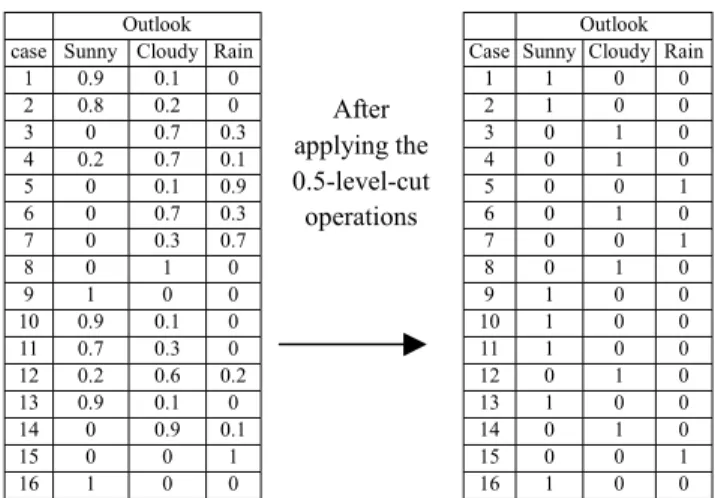
(2) Table 1. A Small Data Set for the Saturday Morning Problem [17] Outlook Temperature Humidity Wind case Sunny Cloudy Rain Hot Mild Cool Humid Normal Windy Not_Windy 1 0.9 0.1 0 1 0 0 0.8 0.2 0.4 0.6 2 0.8 0.2 0 0.6 0.4 0 0 1 0 1 3 0 0.7 0.3 0.8 0.2 0 0.1 0.9 0.2 0.8 4 0.2 0.7 0.1 0.3 0.7 0 0.2 0.8 0.3 0.7 5 0 0.1 0.9 0.7 0.3 0 0.5 0.5 0.5 0.5 6 0 0.7 0.3 0 0.3 0.7 0.7 0.3 0.4 0.6 7 0 0.3 0.7 0 0 1 0 1 0.1 0.9 8 0 1 0 0 0.2 0.8 0.2 0.8 0 1 9 1 0 0 1 0 0 0.6 0.4 0.7 0.3 10 0.9 0.1 0 0 0.3 0.7 0 1 0.9 0.1 11 0.7 0.3 0 1 0 0 1 0 0.2 0.8 12 0.2 0.6 0.2 0 1 0 0.3 0.7 0.3 0.7 13 0.9 0.1 0 0.2 0.8 0 0.1 0.9 1 0 14 0 0.9 0.1 0 0.9 0.1 0.1 0.9 0.7 0.3 15 0 0 1 0 0 1 1 0 0.8 0.2 16 1 0 0 0.5 0.5 0 0 1 0 1. In the Saturday Morning Problem, we have three sports (i.e., Volleyball, Swimming and W_lifting ) to be taken on Saturday morning. This algorithm is now presented as follows: Step 1: Applying the γ-level-cut operations to the values of each attribute, where the threshold value γ is given by the user and γ ∈ [0, 1] . Step 2: According to the results of Step 1, analyze the relationships between the sport plans to be taken and the attributes, respectively, to get the frequency distribution tables for the attributes. Step 3: Translate the frequency distribution tables of the attributes derived in Step 2 into the probability distribution tables, respectively. Step 4: For each sport plan (i.e., Volleyball, Swimming, and W_lifting) according to the probability distribution table for each attribute and based on formula (1), calculate the fuzzy subsethood values between each sport plan and each term of each attribute. Step 5: Generate fuzzy rules based on the fuzzy subsethood values derived in Step 4. If the terms whose fuzzy subsethood values with respect to a sport plan is larger than the level threshold value α, where α ∈ [0, 1] , then these terms will be chosen to form the antecedent parts of the generated fuzzy rules. If there are two terms with fuzzy subsethood values not less than the level threshold value α, then the one with the largest fuzzy subsethood value will be chosen. When a term whose fuzzy subsethold value with respect to a sport plan is equal to the fuzzy subsethood value of the complement of the term with respect to the sport plan, we choose the original term to generate fuzzy rules. If the third rule with respect to the sport plan "W_lifting" can not be generated by the above process, then generate the following rule with respect to the sport plan "W_lifting" shown as follows: Rule 3: IF Degree(Rule 1) < β AND Degree(Rule 2) <β THEN Plan is W_lifting, where Degree(Rule i) means the degree of membership in which the case matches the antecedent part of Rule i, where 1 ≤ i ≤ 2 , β is an applicability threshold value [17] given by the user ,. Step 6:. Volleyball 0 1 0.3 0.9 0 0.2 0 0.7 0.2 0 0.4 0.7 0 0 0 0.8. Plan Swimming 0.8 0.7 0.6 0.1 0 0 0 0 0.8 0.3 0.7 0.2 0 0 0 0.6. W_lifting 0.2 0 0.1 0 1 0.8 1 0.3 0 0.7 0 0.1 1 1 1 0. and β ∈ [0, 1] . Assign weights to the attributes appearing in the antecedent parts of the generated fuzzy rules.. In the following, we apply the proposed algorithm to deal with the Saturday Morning Problem, where we assume that the threshold value γ given by the user is 0.5. [Step 1] Based on Definition 2.2, after applying the 0.5-level-cut to each attribute shown in Table1, we can get the following results as shown in Fig. 1 to Fig. 4. Outlook case Sunny Cloudy Rain 1 0.9 0.1 0 2 0.8 0.2 0 3 0 0.7 0.3 4 0.2 0.7 0.1 5 0 0.1 0.9 6 0 0.7 0.3 7 0 0.3 0.7 8 0 1 0 9 1 0 0 10 0.9 0.1 0 11 0.7 0.3 0 12 0.2 0.6 0.2 13 0.9 0.1 0 14 0 0.9 0.1 15 0 0 1 16 1 0 0. After applying the 0.5-level-cut operations. Outlook Case Sunny Cloudy Rain 1 1 0 0 2 1 0 0 3 0 1 0 4 0 1 0 5 0 0 1 6 0 1 0 7 0 0 1 8 0 1 0 9 1 0 0 10 1 0 0 11 1 0 0 12 0 1 0 13 1 0 0 14 0 1 0 15 0 0 1 16 1 0 0. Fig. 1. Membership grades of the linguistic terms of the attribute "Outlook" after applying the 0.5-level-cut. case 1 2 3 4 5 6 7 8 9 10 11 12 13 14 15 16. Temperature Hot Mild Cool 1 0 0 0.6 0.4 0 0.8 0.2 0 0.3 0.7 0 0.7 0.3 0 0 0.3 0.7 0 0 1 0 0.2 0.8 1 0 0 0 0.3 0.7 1 0 0 0 1 0 0.2 0.8 0 0 0.9 0.1 0 0 1 0.5 0.5 0. After applying the 0.5-level-cut operations. Case 1 2 3 4 5 6 7 8 9 10 11 12 13 14 15 16. Temperature Hot Mild Cool 1 0 0 1 0 0 1 0 0 0 1 0 1 0 0 0 0 1 0 0 1 0 0 1 1 0 0 0 0 1 1 0 0 0 1 0 0 1 0 0 1 0 0 0 1 1 1 0. Fig. 2. Membership grades of the linguistic terms of the attribute "Temperature" after applying the 0.5-level-cut..

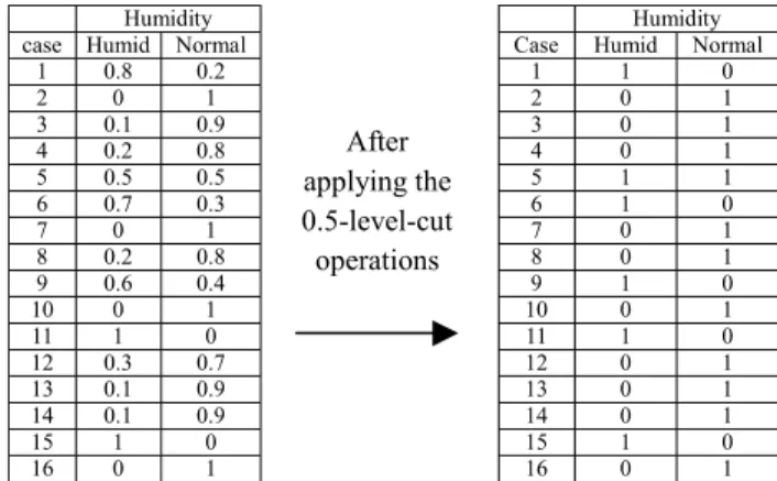
(3) case 1 2 3 4 5 6 7 8 9 10 11 12 13 14 15 16. Humidity Humid Normal 0.8 0.2 0 1 0.1 0.9 0.2 0.8 0.5 0.5 0.7 0.3 0 1 0.2 0.8 0.6 0.4 0 1 1 0 0.3 0.7 0.1 0.9 0.1 0.9 1 0 0 1. After applying the 0.5-level-cut operations. Case 1 2 3 4 5 6 7 8 9 10 11 12 13 14 15 16. Humidity Humid Normal 1 0 0 1 0 1 0 1 1 1 1 0 0 1 0 1 1 0 0 1 1 0 0 1 0 1 0 1 1 0 0 1. Fig. 3. Membership grades of the linguistic terms of the attribute "Humidity" after applying the 0.5-level-cut. case 1 2 3 4 5 6 7 8 9 10 11 12 13 14 15 16. Wind Windy Not_Windy 0.4 0.6 0 1 0.2 0.8 0.3 0.7 0.5 0.5 0.4 0.6 0.1 0.9 0 1 0.7 0.3 0.9 0.1 0.2 0.8 0.3 0.7 1 0 0.7 0.3 0.8 0.2 0 1. After applying the 0.5-level-cut operations. Wind Case Windy Not_Windy 1 0 1 2 0 1 3 0 1 4 0 1 5 1 1 6 0 1 7 0 1 8 0 1 9 1 0 10 1 0 11 0 1 12 0 1 13 1 0 14 1 0 15 1 0 16 0 1. Fig. 4. Membership grades of the linguistic terms of the attribute "Wind" after applying the 0.5-level-cut.. [Step 3] Let's consider the frequency distribution table of the attribute "Outlook" shown in Fig. 5. (1) From the first row of the frequency distribution table shown in Fig. 9, we can see that when Outlook is "Sunny", there are 2 cases in which the sport plan is "Volleyball"; there are 3 cases in which the sport plan is "Swimming"; there are 2 cases in which the sport plan is "W_lifting". Thus, when Outlook is "Sunny", the probability that the spot plan is "Volleyball" is equal to 2 2 = 2+3+ 2 7. ; the probability that the sport plan is. "Swimming". is. equal. to. 3 3 = 2 +3+2 7. ;. the. probability that the sport plan is "W_lifting" is equal to. 2 2 = 2+3+ 2 7. . The results are shown in the. first row of the probability distribution table shown in Fig. 9. (2) From the. second. row of. the. frequency. distribution table shown in Fig. 9, we can see that when Outlook is "Cloudy", there are 3 cases in which the sport plan is "Volleyball"; there is 1. [Step 2] From Fig. 1, we can see that (1) There are 7 cases in which the membership grade of the linguistic term "Sunny" of the attribute "Outlook" is equal to 1, where among 16 cases, there are 2 cases in which the plan is "Volleyball"; there are 3 cases in which the plan is " Swimming"; there are 2 cases in which the plan is "W_lifting". (2) There are 6 cases in which the membership grade of the linguistic term "Cloudy" of the attribute "Outlook" is equal to 1, where among 16 cases, there are 3 cases in which the plan is "Volleyball"; there is 1 case in which the plan is " Swimming"; there are 2 cases in which the plan is "W_lifting". (3) There are three cases in which the membership grade of the linguistic term "Rain" of the attribute "Outlook" is equal to 1, where among 16 cases, there is 0 case in which the plan is "Volleyball"; there is 0 case in which the plan is "Swimming"; there are 3 cases in which the plan is "W_lifting". Thus, we can get the frequency distribution table between the attribute "Outlook" and the sport plan to be taken as shown in the right hand side of Fig. 5. By the same way, we can analyze the relationships between the other attributes and the sport plans to be taken as shown in Fig. 6 to Fig. 8, respectively.. case in which the sport plan is "Swimming"; there are 2 cases in which the sport plan is "W_lifting". Thus, when Outlook is "Cloudy", the probability that the sport plan is "Volleyball" is equal to. 3 3 = 3 +1+ 2 6. ; the probability that the. sport plan is "Swimming" is equal to. 3 1 = 3 +1+ 2 6. ;. the probability that the sport plan is "W_lifting" is equal to. 3 2 = 3 +1+ 2 6. . The results are shown in. the second row of the probability distribution table shown in Fig. 9. (3) From the third row of the frequency distribution table shown in Fig. 9, we can see that when Outlook is "Rain", there is 0 case in which the sport plan is "Volleyball"; there is 0 case in which the sport plan is "Swimming"; there are three cases in which the sport plan is "W_lifting". Thus, when Outlook is "Rain", the probability that the sport plan is "Volleyball" is equal to 0 = 0 0 + 0 + 3. ; the probability that the sport plan.

(4) is "Swimming" is equal to. 0 = 0 0 + 0 + 3. ; the. probability that the sport plan is "W_lifting" is. By the same way, we can derive the probability. equal to. distribution tables for the other attributes as shown in. 3 = 1 0 + 0 + 3. . The results are shown in. the third row of the probability distribution table. case 1 2 3 4 5 6 7 8 9 10 11 12 13 14 15 16. shown in Fig. 9.. Outlook Sunny Cloudy Rain 1 0 0 1 0 0 0 1 0 0 1 0 0 0 1 0 1 0 0 0 1 0 1 0 1 0 0 1 0 0 1 0 0 0 1 0 1 0 0 0 1 0 0 0 1 1 0 0. Volleyball 0 1 0.3 0.9 0 0.2 0 0.7 0.2 0 0.4 0.7 0 0 0 0.8. Plan Swimming 0.8 0.7 0.6 0.1 0 0 0 0 0.8 0.3 0.7 0.2 0 0 0 0.6. W_lifting 0.2 0 0.1 0 1 0.8 1 0.3 0 0.7 0 0.1 1 1 1 0. Fig. 10 to Fig. 12.. Frequency Distribution Table Outlook Sunny Cloudy Rain Volleyball 1 0 0 2 0 1 0 3 0 0 1 0. Plan Swimming 3 1 0. W_lifting 2 2 3. Fig. 5. Frequency distribution table between the attribute "Outlook" and the sport plans to be taken.. Case 1 2 3 4 5 6 7 8 9 10 11 12 13 14 15 16. Hot 1 1 1 0 1 0 0 0 1 0 1 0 0 0 0 1. Temperature Mild Cool 0 0 0 0 0 0 1 0 0 0 0 1 0 1 0 1 0 0 0 1 0 0 1 0 1 0 1 0 0 1 1 0. Volleyball 0 1 0.3 0.9 0 0.2 0 0.7 0.2 0 0.4 0.7 0 0 0 0.8. Plan Swimming 0.8 0.7 0.6 0.1 0 0 0 0 0.8 0.3 0.7 0.2 0 0 0 0.6. W_lifting 0.2 0 0.1 0 1 0.8 1 0.3 0 0.7 0 0.1 1 1 1 0. Frequency Distribution Table Temperature Hot Mild Cool 1 0 0 0 1 0 0 0 1. Volleyball 2 3 1. Plan Swimming 4 0 0. W_lifting 1 2 4. Fig. 6. Frequency distribution table between the attribute " Temperature" and the sport plans to be taken.. Case 1 2 3 4 5 6 7 8 9 10 11 12 13 14 15 16. Humidity Humid Normal 1 0 0 1 0 1 0 1 1 1 1 0 0 1 0 1 1 0 0 1 1 0 0 1 0 1 0 1 1 0 0 1. Volleyball 0 1 0.3 0.9 0 0.2 0 0.7 0.2 0 0.4 0.7 0 0 0 0.8. Plan Swimming 0.8 0.7 0.6 0.1 0 0 0 0 0.8 0.3 0.7 0.2 0 0 0 0.6. W_lifting 0.2 0 0.1 0 1 0.8 1 0.3 0 0.7 0 0.1 1 1 1 0. Frequency Distribution Table Humidity Humid Normal 1 0 0 1. Volleyball 0 5. Plan Swimming 3 1. Fig. 7. Frequency distribution table between the attribute " Humidity" and the sport plans to be taken.. W_lifting 3 5.

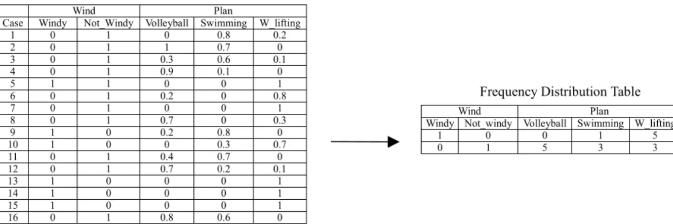
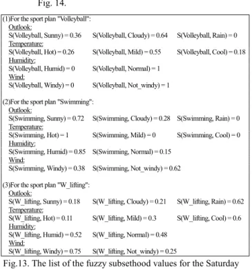
(5) Case 1 2 3 4 5 6 7 8 9 10 11 12 13 14 15 16. Windy 0 0 0 0 1 0 0 0 1 1 0 0 1 1 1 0. Wind Not_Windy 1 1 1 1 1 1 1 1 0 0 1 1 0 0 0 1. Volleyball 0 1 0.3 0.9 0 0.2 0 0.7 0.2 0 0.4 0.7 0 0 0 0.8. Plan Swimming 0.8 0.7 0.6 0.1 0 0 0 0 0.8 0.3 0.7 0.2 0 0 0 0.6. W_lifting 0.2 0 0.1 0 1 0.8 1 0.3 0 0.7 0 0.1 1 1 1 0. Frequency Distribution Table Wind Windy Not_windy 1 0 0 1. Volleyball 0 5. Plan Swimming 1 3. W_lifting 5 3. Fig. 8. Frequency distribution table between the attribute "Wind" and the sport plans to be taken. Frequency Distribution Table Outlook Sunny Cloudy Rain 1 0 0 0 1 0 0 0 1. Volleyball 2 3 0. Plan Swimming 3 1 0. Probability Distribution Table W_lifting 2 2 3. Outlook Sunny Cloudy Rain Volleyball 1 0 0 2/7 0 1 0 3/6 0 0 1 0. Plan Swimming 3/7 1/6 0. W_lifting 2/7 2/6 1. Fig. 9. Derive the probability distribution table of the attribute "Outlook". Frequency Distribution Table Temperature Hot Mild Cool 1 0 0 0 1 0 0 0 1. Volleyball 2 3 1. Plan Swimming 4 0 0. Probability Distribution Table W_lifting 1 2 4. Temperature Hot Mild Cool 1 0 0 0 1 0 0 0 1. Volleyball 2/7 3/5 1/5. Plan Swimming 4/7 0 0. W_lifting 1/7 2/5 4/5. Fig. 10. Derive the probability distribution table of the attribute "Temperature". Frequency Distribution Table Humidity Humid Normal 1 0 0 1. Volleyball 0 5. Plan Swimming 3 1. Probability Distribution Table W_lifting 3 5. Humidity Humid 1 0. Normal 0 1. Plan Volleyball 0 5/11. Swimming 3/6 1/11. W_lifting 3/6 5/11. Fig. 11. Derive the probability distribution table of the attribute "Humidity". Probability Distribution Table. Frequency Distribution Table Wind Windy Not_windy 1 0 0 1. Volleyball 0 5. Plan Swimming 1 3. W_lifting 5 3. Wind Windy Not_windy 1 0 0 1. Volleyball 0 5/11. Plan Swimming 1/11 3/11. W_lifting 5/11 3/11. Fig. 12. Derive the probability distribution table of the attribute "Wind". [Step 4] Using formula (1), we can calculate the subsethood values between each sport plan and attribute. For example, based on the probability distribution table of the attribute "Outlook" shown in Fig. 9, we can calculate the fuzzy subsethood value S(Volleyball, Sunny) between "Volleyball" and "Sunny" shown as follows: M(Volleyba ll ∩ Sunny) = min(2/7, 1) + min(3/6, 0) + min(0, 0) = 2/7 + 0 + 0 = 0.28, M(Volleyba ll). = 2/7 + 3/6 + 0 = 0.78,. S(Volleyball, Sunny) = M(Volleyba ll ∩ Sunny) M(Volleyba ll) 2/7. = 2 / 7 + 3 / 6 + 0 = 0.36. By the same way, based on Figs.9-12, we can get the list of the fuzzy subsethood values for the Saturday Morning Problem as shown in Fig. 13. [Step 5] After we get subsethood values between each sport plan (i.e., Volleyball, Swimming, and W_lifting) and each term of each attribute, we can select the terms of. attributes for each sport plan to form a rule. We select the terms of the attributes with the highest subsethood values with respect to the sport plan to form the antecedent part of the rule for each sport plan, and we use the sport plan to form the consequence part of the rule. We use a level threshold value α to decide whether we want to select the terms of attributes or not, where the level threshold value α is between 0 and 1 and is given by the user. We also consider the fuzzy subsethood values of the complement of the terms of the attributes for each sport plan. We choose the terms of the attributes whose fuzzy subsethood values are not less than the level threshold value α, where α ∈ [0, 1] . If there are two terms with fuzzy subsethood values not less than the level threshold value α, then the one with largest fuzzy subsethold value will be chosen. When a term whose fuzzy subsethood value with respect to the sport plan is equal to the fuzzy subsethold value of the complement of the term with respect to the sport plan, we choose the original term to generate fuzzy rules. For example, from Fig. 13, we can see that the fuzzy.

(6) subsethold values of the terms of the attributes with respect to the sport plan "Volleyball" are as shown in Fig. 14. (1)For the sport plan "Volleyball": Outlook: S(Volleyball, Sunny) = 0.36 S(Volleyball, Cloudy) = 0.64 S(Volleyball, Rain) = 0 Temperature: S(Volleyball, Hot) = 0.26 S(Volleyball, Mild) = 0.55 S(Volleyball, Cool) = 0.18 Humidity: S(Volleyball, Humid) = 0 S(Volleyball, Normal) = 1 Wind: S(Volleyball, Windy) = 0 S(Volleyball, Not_windy) = 1 (2)For the sport plan "Swimming": Outlook: S(Swimming, Sunny) = 0.72 S(Swimming, Cloudy) = 0.28 S(Swimming, Rain) = 0 Temperature: S(Swimming, Hot) = 1 S(Swimming, Mild) = 0 S(Swimming, Cool) = 0 Humidity: S(Swimming, Humid) = 0.85 S(Swimming, Normal) = 0.15 Wind: S(Swimming, Windy) = 0.38 S(Swimming, Not_windy) = 0.62 (3)For the sport plan "W_lifting": Outlook: S(W_lifting, Sunny) = 0.18 Temperature: S(W_lifting, Hot) = 0.11 Humidity: S(W_lifting, Humid) = 0.52 Wind: S(W_lifting, Windy) = 0.75. S(W_lifting, Cloudy) = 0.21. S(W_lifting, Rain) = 0.62. S(W_lifting, Mild) = 0.3. S(W_lifting, Cool) = 0.6. S(W_lifting, Normal) = 0.48 S(W_lifting, Not_windy) = 0.25. Fig.13. The list of the fuzzy subsethood values for the Saturday Morning Problem [17] Assume that the level threshold value α given by the user is 0.9 (i.e., α = 0.9). From Fig. 14, we can see that only S(Volleyball, NOT Rain) is not less than 0.9, so we add "Outlook is Not Rain" into the antecedent part of the rule. We can't find any terms of the attribute "Temperature" whose fuzzy subsethood values is larger than 0.9, so the terms of the attribute "Temperature" can be ignored. The third attribute "Humidity" has two terms (i.e., NOT Humid and Normal) whose fuzzy subsethood values S(Volleyball, NOT Humid) and S(Volleyball, Normal) are larger than 0.9, we choose the original term "Normal" and add "Humidity is Normal" into the antecedent part of this rule. The attribute "Wind" has a term "Not_Windy" whose fuzzy subsethood value is larger than 0.9, so we choose the term "Not_windy" of the attribute "Wind" and add "Wind is Not_windy" to the antecedent part of the rule. Thus, we can get the rule for the sport plan "Volleyball" shown as follows: Rule 1: IF Outlook is Not Rain ANDHumidity is Normal AND Windy is Not_Windy THEN Plan is Volleyball. From Fig. 13, we also can see that the fuzzy subsethood values of the terms of the attributes with respect to the sport plan "Swimming" are shown as in Fig. 15. From Fig. 15, we can see that only S(Volleyball, NOT Rain) is not less than 0.9, so we add "Outlook is Not Rain" into the antecedent part of the rule. The second attribute "Temperature" has three terms (i.e., Hot and NOT Mild, and NOT Cool) whose fuzzy subsethood values S(Volleyball, Hot), S(Volleyball, NOT Mild), and S(Volleyball, NOT Cool) are larger than 0.9, we choose. the term "Hot" and add "Temperature is Hot" into the antecedent part of the rule due to fact that the term "Hot" has the largest fuzzy subsethood value with respect to the sport plan "Swimming" among the terms "Hot", "Not Mild", and "Not Cool". We can't find any terms of the attributes "Humidity" and "Wind" whose fuzzy subsethood values is larger than 0.9, so the terms of the attribute "Humidity" and "Wind" can be ignored. Thus, we can get the rule for the sport plan "Swimming" shown as follows: Rule 2: IF Outlook is Not Rain ANDTemperature is Hot THEN Plan is Swimming. From Fig. 13, we also can see that the fuzzy subsethood values of the terms of the attributes with respect to the sport plan "W_lifting" are shown as in Fig. 16. From Fig. 16, we can't find any terms of the attributes "Outlook", "Temperature", "Humidity", and "Wind" whose fuzzy subsethood values with respect to the sport plan "W_lifting" is larger than 0.9. Thus, in this situation, we can’t generate the third rule for the sport plan "W_lifting" shown as follows: Rule 3: IF Degree(Rule 1) < β AND Degree(Rule 2) < β THEN Plan is W_lifting, where β is an applicability threshold value given by the user and β ∈ [0, 1] . In summary, if the retrieval threshold value α= 0.9 and the applicability threshod value β = 0.6 then we can get the following fuzzy rules which are the same as the ones of Chen-Lee-Lee's method [5]: Rule 1: IF Outlook is NOT Rain AND Humidity is Normal And Wind is Not-windy THEN Plan is Volleyball Rule 2: IF Outlook is Not Rain AND Temperature is Hot THEN Plan is Swimming Rule 3: IF Degree(Rule 1) < β AND Degree(Rule 2) < β THEN Plan is W_lifting. S(Volleyball, Sunny) = 0.36 S(Volleyball, Hot) = 0.26 S(Volleyball, Humid) = 0 S(Volleyball, Windy) = 0. S(Volleyball, Cloudy) = 0.64 S(Volleyball, Mild) = 0.55 S(Volleyball, Normal) = 1 S(Volleyball, Not_windy) = 1. S(Volleyball, Rain) = 0 S(Volleyball, Cool) = 0.18. Fig. 14. Fuzzy subsethood values of the terms of attributes with respect to the sport plan "Volleyball". S(Swimming, Sunny) = 0.72 S(Swimming, Hot) = 1 S(Swimming, Humid) = 0.85 S(Swimming, Windy) = 0.38. S(Swimming, Cloudy) = 0.28 S(Swimming, Rain) = 0 S(Swimming, Mild) = 0 S(Swimming, Cool) = 0 S(Swimming, Normal) = 0.15 S(Swimming, Not_windy) = 0.62. Fig. 15. Fuzzy subsethood values of the terms of attributes with respect to the sport plan "Swimming". S(W_lifting, Sunny) = 0.18 S(W_lifting, Hot) = 0.11 S(W_lifting, Humid) = 0.52 S(W_lifting, Windy) = 0.75. S(W_lifting, Cloudy) = 0.21 S(W_lifting, Rain) = 0.62 S(W_lifting, Mild) = 0.3 S(W_lifting, Cool) = 0.6 S(W_lifting, Normal) = 0.48 S(W_lifting, Not_windy) = 0.25. Fig. 16. Fuzzy subsethood values of the terms of attributes with respect to the sport plan "W_lifting". [Step 6] This step assigns weights to the attributes appearing in the antecedent parts of the generated fuzzy rules. Each attribute appearing in the antecedent parts of the generated fuzzy rules may have different important degrees, so we assign a weight to each attribute appearing in the antecedent parts of the generated fuzzy.

(7) rules. From Step 5, we can get two fuzzy rules Rule 1 and Rule 2 shown as follows: Rule 1: IF Outlook is Not Rain AND Humidity is Normal AND Wind is Not_Windy THEN Plan is Volleyball Rule 2: IF Outlook is Not Rain AND Temperature is Hot THEN Plan is Swimming In Rule 1, if we let the weights of the attributes "Outlook", "Humidity", and "Wind" be 0.3, 0, and 0.7, respectively, and in Rule 2, if we let the weights of the attributes "Outlook" and "Temperature" be 0.1 and 0.9, respectively, then we let Degree(Rule i) = Degree(sport plan i), where 1 ≤ i ≤ 2 , sport plan i is the sport plan of Rule i, and Degree(Rule i) means the degree of membership. Then, we assign weights to the attributes appearing in the antecedent part of Rule 1 as follows: Degree(Volleyball)= Degree(Not Rain) * 0.3 + Degree(Normal) * 0 + Degree(Not_Windy) * 0.7 = Degree(Not Rain) * 0.3 + Degree(Not_Windy) * 0.7. Next, we assign weights to the attributes appearing in the antecedent part of Rule 2 as follows: Degree(Swimming)=Degree(Not Rain) * 0.1 + Degree(Hot) * 0.9. Then, we can assign Degree(Rule 1) = Degree(Volleyball), Degree(Rule 2) = Degree(Swimming). For example, we can calculate Case 13 of Table 1 shown as follows: Degree(Volleyball) = Degree(Not Rain) * 0.3 + Degree(Not_Windy) * 0.7 = (1- 0) * 0.3 + 0 * 0.7 = 0.3, Degree(Swimming) = Degree(Not Rain) * 0.1+ Degree(Hot) * 0.9 = (1- 0) * 0.1 + 0.2 * 0.9 = 0.28, Degree(Rule 1) = Degree(Volleyball) = 0.3, Degree(Rule 2) = Degree(Swimming) = 0.28. When Rule 1 and Rule 2 can’t classify well for Case 13 of Table 1 (i.e., Case 13 belonging to the sport plans “Volleyball” and “Swimming” have low degrees of membership), we can then classify Case 13 into the sport plan “W_lifting”. In this situation, we need to use an applicability threshold value β given by the user, where β ∈[0, 1] , to decide the suitability of existing classification fuzzy rules. If Degree(Rule i) ≥ β , where i∈{1, 2 , ..., n} and n is the number of the existing classification fuzzy rules, then Rule i is suitable to classify this case. Thus, we generate the third rule as follows: Rule 3: IF Degree(Rule 1) < β AND Degree(Rule 2) < β THEN Plan is W_lifting. That is, if Degree(Rule 1) and Degree(Rule 2) are less than β, where β is an applicability threshold value given by the user and β ∈[0, 1] , then we set the value of Degree(W_lifting) to 1. Otherwise, we assign 0 to Degree(W_lifting).. Now we calculate Case 13 of Table 1 again, and we assume that the applicability threshold value β given by user is 0.725. Thus, we can get the classification result shown as follows: Degree(Volleyball) = Degree(Not Rain) * 0.3 + Degree(Not_Windy) * 0.7 = (1- 0) * 0.3 + 0 * 0.7 = 0.3, Degree(antecedent part of Rule 2) = Degree(Not Rain) * 0.1 + Degree(Hot) * 0.9 = (1- 0) * 0.1 + 0.2 * 0.9 = 0.28, Degree(Rule 1) = Degree(Volleyball) = 0.3, Degree(Rule 2) = Degree(Swimming) = 0.28. According to Rule 3, Because Degree(Rule 1) < 0.725 and Degree(Rule2) < 0.725, we can see that Case 13 of Table 1 is classified into the sport plan "W_lifting" (i.e., Degree(Rule 3) = Degree(W_lifting) = 1). Assume that the applicability threshold value β given by the user is 0.725. After we apply the generated weighted fuzzy rules to 16 cases of the "Saturday Morning Problems", we can get 100% classification accuracy rate as shown in Table 2, where the calculations for Case 1 are shown as follows: Degree(Rule 1) = Degree(Volleyball) = Degree(Not Rain) * 0.3 + Degree(Not_Windy) * 0.7 = (1 - 0) * 0.3 + 0.9 * 0 + 0.6 * 0.7 = 0.72, Degree(Rule 2) = Degree(Swimming) = Degree(Not Rain) * 0.1 + Degree(Hot) * 0.9 = (1 - 0) * 0.1 + 1 * 0.9 = 1. Because Degree(Rule 1) < 0.725 and Degree(Rule 2) > 0.725, based on Rule 3, we can see that Degree(W_lifting) = 0. Thus, if we let the weights of the attributes "Outlook", "Humidity" and "Wind" of Rule 1 be 0.3, 0 and 0.7, respectively, and we let the weights of the attributes "Outlook" and "Temperature" of Rule 2 be 0.1 and 0.9, respectively, where the level threshold value α = 0.9 and the applicability threshold value β = 0.725, we can get 100% classification accuracy rate and it has the smallest total Euclidian Distance between the classification result of the generated weighted fuzzy rules and known classification in the training data, where the generated weighted fuzzy rules are shown as follows: Rule 1: IF Outlook is Not Rain (Weight = 0.3) AND Humidity is Normal (Weight = 0) AND Wind is Not_Windy (Weight = 0.7) THEN Plan is Volleyball Rule 2: IF Outlook is Not Rain (Weight = 0.1) AND Temperature is Hot (Weight = 0.9) THEN Plan is Swimming Rule 3: IF Degree(Rule 1) < 0.725 AND Degree(Rule 2) < 0.725 THEN Plan is W_lifting.

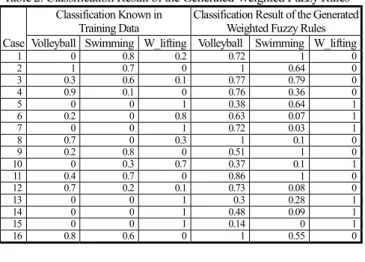
(8) 4. CONCLUSIONS In this paper, we have presented a new method to generate weighted fuzzy rules from numerical data to deal with the Saturday Morning Problem [17]. The proposed method calculates the fuzzy subsethood values between the terms of attributes and the sport plans to be made, and it uses the γ-level-cut, the level threshold value α, and the applicability threshold value β to generate weighted fuzzy rules, where γ, α and β are given by the user, γ ∈ [0, 1] , α ∈ [0, 1] , and β ∈ [0, 1] . There are 45 ways to assign different weights to different attributes appearing in the antecedent parts of the generated weighted fuzzy rules which all can get 100% classification accuracy rate. We also can see that if we let the weights of the attributes "Outlook", "Humidity" and "Wind" of Rule 1 be 0.3, 0 and 0.7, respectively, and if we let the weights of the attributes "Outlook" and "Temperature" of Rule 2 be 0.1 and 0.9, respectively, we can get 100% classification accuracy rate (under γ=0.5, α = 0.9, and β = 0.725), where it has the smallest total Euclidian distance between the classification result of the generated weighted fuzzy rules and the known classification in the training data. The proposed method is better than Yuan-and-Shaw's method presented in [17] and Chen-LeeLee's method presented in [5] due to the fact that the classification accuracy rate of the proposed method is 100%, but the classfication accuracy rate of Yuan-and-Shaw's method presented in [17] is 81.25%, and the classification accuracy rate of Chen-Lee-Lee's method persented in [5] is 93.75%. Table 2. Classification Result of the Generated Weighted Fuzzy Rules Classification Known in Classification Result of the Generated Training Data Weighted Fuzzy Rules Case Volleyball Swimming W_lifting Volleyball Swimming W_lifting 1 2 3 4 5 6 7 8 9 10 11 12 13 14 15 16. 0 1 0.3 0.9 0 0.2 0 0.7 0.2 0 0.4 0.7 0 0 0 0.8. 0.8 0.7 0.6 0.1 0 0 0 0 0.8 0.3 0.7 0.2 0 0 0 0.6. 0.2 0 0.1 0 1 0.8 1 0.3 0 0.7 0 0.1 1 1 1 0. 0.72 1 0.77 0.76 0.38 0.63 0.72 1 0.51 0.37 0.86 0.73 0.3 0.48 0.14 1. 1 0.64 0.79 0.36 0.64 0.07 0.03 0.1 1 0.1 1 0.08 0.28 0.09 0 0.55. 0 0 0 0 1 1 1 0 0 1 0 0 1 1 1 0. ACKNOWLEDGEMENTS This work was supported in part by the National Science Council, Republic of China, under Grant NSC 89-2213-E-011-060. REFERENCES [1] D. G. Burkhardt and P. P. Bonissone, "Automated fuzzy knowledge base generation and turning," Proceedings of the 1992 IEEE International Conference on Fuzzy Systems, San Diego, California, pp. 179-188, 1992 [2] J. L. Castro, J. J. Castro-Schez, and J. M. Zurita, "Learning maximal structure rules in fuzzy logic for knowledge acquisition in expert systems," Fuzzy Sets and Systems, vol. 101, no. 3, pp. 331-342, 1999. [3] J. Cendrowska, "PRISM: an algorithm for inducing modular rules," International Journal Man-Machine Studies, vol. 27,. no. 3, pp. 349-370, 1987. [4] S. M. Chen and M. S. Yeh, "Generating fuzzy rules from relational database systems for estimating null values," Cybernetics and Systems: An International Journal, vol. 28, no. 8, pp. 695-723, 1997. [5] S. M. Chen, S. H. Lee, and C. H. Lee, "Generating fuzzy rules from numerical data for handling fuzzy classification problems," Proceedings of the 1999 National Computer Symposium, Taipei, Taiwan, Republic of China, vol. 2, pp. 336-343, 1999. [6] T. P. Hong, and J. B. Chan, "Finding relevant attributes and membership functions," Fuzzy Sets and Systems, vol. 103, no. 3, pp. 389-404, 1999. [7] T. P. Hong, and C. Y. Lee, "Introduction of fuzzy rules and membership functions from training examples," Fuzzy Sets and Systems, vol. 84, no. 1, pp. 33-47, 1996. [8] B. Kosko, "Fuzzy entropy and conditioning," Information Sciences, vol. 40, no. 2, pp. 165-174, 1986. [9] H. Nomura, I. Hayashi, and N. Wakami, "A learning method of fuzzy inference ruled by descent method," Proceedings of the 1992 IEEE International Conference on Fuzzy systems, San Diego, California, pp. 203-210,1992. [10] T. Sudkamp and R. J. Hammell II, "Interpolating, complete, and learning fuzzy rules," IEEE Transactions on Systems, Man, and Cybernetics, vol. 24, no. 2, pp. 332-342, 1994. [11] T. Takagi and M. Sugeno, "Fuzzy identification of systems and its applications to modeling and control," IEEE Transactions on Systems, Man, and Cybernetics, vol. 15, no. 1, pp. 116-132, 1985. [12] L. X. Wang and J. M. Mendel, "Generating fuzzy rules by learning from examples," IEEE Transactions on Systems, Man, and Cybernetics, vol. 22, no. 6, pp. 1414-1427, 1992. [13] X. Wang, B. Chen, G. Qian, and F. Ye, "On the optimization of fuzzy decision tree," Fuzzy Sets and Systems, vol. 112, no. 1, pp. 117-125, 2000. [14] X. Wang, and J. Hong, "Learning optimization in simplifying fuzzy rules," Fuzzy Sets and System, vol. 106, no. 3, pp. 349-356, 1999. [15] C. H. Wang, J. F. Liu, T. P. Hong, S. S. Tseng, "A fuzzy inductive learning strategy for modular rules," Fuzzy Sets and System, vol. 103, no. 1, pp. 91-105, 1999. [16] T. P. Wu and S. M. Chen, "A new method for constructing membership functions and fuzzy rules from training examples," IEEE Transactions on Systems, Man, and Cybernetics, vol. 29, no. 1, pp. 25-40, 1999. [17] Y. Yuan, and M. J. Shaw, "Induction of fuzzy decision trees," Fuzzy Sets and Systems, vol. 69, no. 4, pp.125-139, 1995. [18] L. A. Zadeh, "Fuzzy sets," Information and Control, vol. 8, pp. 338-353, 1965. [19] L. A. Zadeh, "Fuzzy logic," IEEE Computer, vol. 21, no. 4, pp. 89-91, 1988. [20] L. A. Zadeh, "The concept of a linguistic variable and its application to approximate reasoning - I," Information Sciences, vol. 8, no. 3, pp. 199-249, 1975. [21] H. J. Zimmermann, Fuzzy Set Theory and Its Applications. Boston: Kluwer Academic Publisher, 1991..

(9)