Abstract
The accuracy of a finite element simulation depends mostly on the mesh model. Many parameters influence the precision of a finite element mesh. In orthopedic biomechanics, the material property of bone is one of the major parameters in the simulation, especially the heterogeneous of cortex and cancellous bone. The common approach to simulate the heterogeneous of bone is to model with several sets of elastic modulus for the bone material. However, the required set numbers of elastic modulus to obtain a feasible solution is still unclear for bone structure. The objective of this study was therefore to investigate the necessary of heterogeneous femoral material for finite element simulation. Three rabbit femora were selected as the target subjects and three-point bending test was used as the loading mode. Experimental measurement of the displacement value under the three-point bending test was used as the reference point for justification the analytical results and convergence. The results indicated that the displacement value decreased as the set number of cortex elastic modulus reduced. To achieve a 5% absolute convergence for displacement, a minimum of 60 sets of cortex bone elastic modulus is required.
Keywords: Finite element method, Femur, Heterogeneous, Three-point bending test.
Introduction
Since Breakelmans first introduced the finite element analysis for spinal simulation in 1972, the finite element method has become an important research tool in orthopedic biomechanics. Finite element method, comparing with the experimental approach, can provide comprehensive predication of the full field mechanical indices and allow effective control of the investigated parameters in the analysis thus is suitable for studying the biomechanical rational of orthopedic structures. With the advance of computer power, the applications of finite element simulation have been ext ended to the field of non-linearity such as the investigation of the bone fixation system [1], evaluation of fracture risk for osteoporosis [2,3] or even predication of bone remodeling after total hip replacement [4]. The efficiency of the finite element analysis depends on the finite element models. However, the process of setting up the finite element models in orthopedic applications still lacks a rigid guideline.
In early orthopedic applications, two-dimensional models were the major approaches due to the limitations in computer capacities and the relative ease in setting up the geometry * Corresponding author: Chih-Han Chang
Tel: +886-6-2757575 ext. 63427; Fax: +886-6-2343270 E-mail: [email protected]
and loading conditions [5,6]. These simplified models are difficulty to provide valuable clinical information. Recently, three-dimensional approaches have become the major trend for orthopedic finite element simulation [3,7,8]. The typical procedures to setup a three-dimensional mesh model, especially for the bone structure, is to employ CT images. Nodes are placed on the boundaries of bone structure with hand-digitizer or simple interval dividing programs [8]. Corresponding nodes between CT slices are then connected to form three-dimensional elements. These processes not only require intensive labor efforts but also produce ill-conditioned elements. With the advent of computer graphics techniques and computer aided design systems, many algorithms were developed to generate the three-dimensional bone mesh with less human interaction and offer better element shape.
Even with the better approximation in bone geometry by these semi-automatic mesh generators, the properties of bone material still provide obstacles in setting up a realistic finite element bone mesh. The bone material has been recognized as nonlinear, anisotropy and non-homogeneity; but in most finite element models, the bone material is generally modeled as linear, isotropy and assigned with only two material moduli, that is cortex and cancellous [5,6]. The nonlinear and anisotropic characteristics of the bone material are still difficulty to be simulated in finite element models
Figure 1. Schematic plot of the three-point bending test
Figure 2. The finite element mesh model to simulate the three-point bending at current stage. The heterogeneous property of bone is possible
to be modeled with finite number of elastic modulus based on the CT data. The objective of this study was therefore to investigate the heterogeneous modeling of bone material for finite element analysis. To justify the simulated results, displacement measurements of rabbit femora using three-point bending test were employed as the absolute convergent reference point.
Material and Methods
Three major phases were included in this study. Firstly, rabbit femora were used to execute the three-point bending experiments and the force-displacement curves were recorded to setup the reference for the validation of finite element simulations. After that, three-dimensional finite element models for the corresponding three-point bending tests were generated by a self-develop of program based on CT section images [9]. Bone material properties of these models were assigned by the power law relationship between elastic modulus and CT numbers [7]. Finally, various numbers of bone material, simulated with different elastic modulus, were applied in the finite element models to evaluate the effect of non-homogeneous bone material.
Three-point Bending Test
Three rabbit femora were used in this study including two normal femora and an osteopropostic femur induced by immobilization. After sacrifice of the rabbits, the soft -tissue
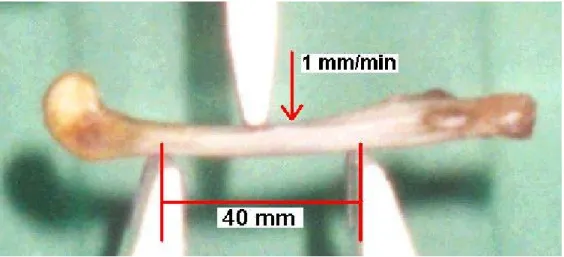
were stripped from the femora and scanned with GE fast CT (General Electric Co., USA) with 1mm slice interval and 512x512 resolution at 15mm of field of scan (FOS). In order to maintain the bone quality, the three-point bending test was performed within 1hr after each sacrificing. Before the test, each femur was warped by wet clothes and stored inside a sealed container. The experimental set up of the three-point bending test was shown in Figure 1. The loading speed was set at 1mm/min till fracture. The force-displacement curves of the three femora were recoded as the reference for finite element validation.
Three-dimensional Finite Element Mesh
For the three femora, three dimensional mesh models were generated through a self-develop of program based on the CT images of each femur [11]. In order to have an accurate approximation in the femoral geometry, the average element size for the tetrahedron elements was less than 0.6 mm. Figure 2 shows one of the three mesh models. To better simulate the three-point bending test for finite element analysis, three markers were placed on each femur before CT scanning to identify the three loading locations during bending test (Figure 3). These markers detectable in the CT images were used in each mesh model to setup the loading and constrained boundary conditions in the three-point bending simulation. The nodes at the two lower positioned markers were fixed in all directions as the boundary condition; while the node matched the upper marker position was loaded by a concentration downward force of 136.3N is one step as show in figure 2.
(a)
(b)
Figure 3. (a) The rabbit femur with three markers to identify the locations for the three-point test. (b) The CT image of rabbit femur with the marker observed.
Assignment of modulus of Elasticity
Many studies have revealed that there is a power relationship between the elastic modulus and the apparent density of bone material, and a linear correlation between the apparent density and CT number [3,7,12]. In this study, the elastic modulus of each tetrahedron element was derived from the CT numbers at its four nodes based on the following equation:
E = A*(CT/100) B (1) where E: elastic modulus, CT: CT number and A, B: material parameters.
The elastic modulus of each node, with its CT number obtained from the CT images, was calculated from above equation and the elastic modulus of a tetrahedron element was acquired from the averaged elastic modulus of the four nodes that construct this element. The values of parameters A and B for each femur were obtained by a trail and error approach to
match the displacement measured from the three-point bending test and the finite element simulation on that particular femur.
To study the non-homogeneous effect of bone material in the finite element models, fourteen groups of various numbers of elastic modulus were setup as shown in Table 1. Within the table, X stands for the number of cortex bone materials and Y identifies the number of spongy bone materials used in each femoral model. The CT range of cortex bone was assigned between 1500 and 3000 and the CT range of cancellous bone was assigned within 800 to 1500. Therefore, in the first group of Table 1, each CT number has a corresponding elastic modulus and this is the most non-homogeneous model available within the resolution of CT. The last (fourteenth) group of Table 1 would only have one material for cortex and one for cancellous respectively and this represents the most homogeneous model. The Poisson’s ratio for all materials was assigned to 0.3 as referred from literatures [8, 9]. All materials were assumed to be linear elastic.
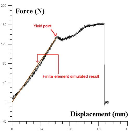
Figure 4. The force-displacement curve of a rabbit femur under three-point bending test and finite element simulated results
Table 1. Fourteen groups of different levels of heterogeneous femur models were setup. The first group represents the highest level of heterogeneous and the level of heterogeneous decreased as the group number increased.
Group Cortical bone material numbers (X) Cancellous bone material numbers (Y) Displacement (mm) 1 2000 700 0.625 2 1000 350 0.624 3 500 175 0.622 4 250 88 0.618 5 200 70 0.616 6 125 44 0.611 7 63 22 0.597 8 32 11 0.571 9 20 7 0.545 10 16 6 0.525 11 8 4 0.455 12 4 2 0.359 13 2 1 0.253 14 1 1 0.156 0 0.1 0.2 0.3 0.4 0.5 0.6 0.7 0 1 2 3 4 5 6 7 8 9 10 11 12 13 14 15 Group Displacement (mm) Results
Figure 4 shows the force-displacement curve of a femur under three-point bending test and the fracture force of this femur was 162.5 N. The yield point was determined at the end of the linear portion of the curve and the values for yield force and displacement were 136.3 N and 0.624 mm, respectively. With these measured values, the parameters of A and B in the equation for elastic modulus could be determined for the group one (the most non-homogenous) model, i.e., with 2000 cortex materials and 700 cancellous materials. Two sets of A and B (A=7.74, B=2.0 and A=4.09, B=2.2) were obtained by the trail- Figure 5. The displacement values decreased as the level of heterogeneous
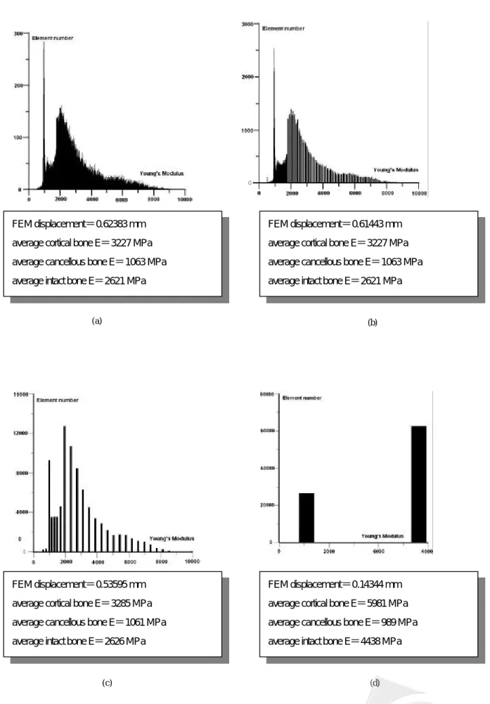
Figure 6. The histogram of number of elements for each elastic modulus in (a)group 1 (b)group 5 (c)group 9 (d)group 14 FEM displacement=0.62383 mm
average cortical bone E=3227 MPa average cancellous bone E=1063 MPa average intact bone E=2621 MPa
FEM displacement=0.61443 mm average cortical bone E=3227 MPa average cancellous bone E=1063 MPa average intact bone E=2621 MPa
FEM displacement=0.53595 mm average cortical bone E=3285 MPa average cancellous bone E=1061 MPa average intact bone E=2626 MPa
FEM displacement=0.14344 mm average cortical bone E=5981 MPa average cancellous bone E=989 MPa average intact bone E=4438 MPa
(a) (b)
with the experimental yield point.
For the first set of parameters, A=7.74 and B=2.0, the displacement value equals 0.625mm (under 136.3N force) which indicates a acceptable simulated result as compared to the experimental yield point as show in figure 4. However, as the numbers of elastic modulus reduced in each material group simulation, the displacement values decreased (under the same 136.3N loading) as shown in Table 1 and figure 5. It is observed that as the number of elastic modulus was less than 20 for the cortex, the displacement demonstrates a significant decreasing. To achieve a 5% convergence for displacement the number of cortex elastic modulus should greater than 60.
For the second set of parameters, A=4.09 and B=2.2, and the rest two femora, the results were similar, i.e., as the number of elastic modulus reduced in the simulation, the displacement decreased (under the same loading) and the minimum number of cortex elastic modulus should greater than 60 in order to achieve a 5% convergence in displacement.
Discussion and Conclusion
Three factors affect the accuracy of a finite element model, i.e., the geometry, the material and the loading (including boundary) conditions. In this study , with better approximation in geometry and loading condition, the heterogeneous of femur was evaluated to justify its influence.
When the elastic modulus is converted from CT number, which is the general approach adopted by most finite element researches, under the same loading force, the displacement decreased as the number of cortex elastic modulus reduced. To explain the results, the histograms of the elastic modulus distributions of four material groups were shown in Figure 6. For the group one model, the highest level of heterogeneous, the simulated displacement value was identical to that of the experiment and the averaged elastic modulus for the cancellous, cortex and the whole femur were 1063Mpa, 3277Mpa and 2621Mpa, respectively. For the model with 200 cortex materials and 70 cancellous materials, there was roughly 1% of error in the displacement outcome. However, for the model with only 20 cortex and 7 cancellous materials, the displacement error was greater than 10% while the difference in averaged elastic modulus (compared with group one) was less than 1% (1061Mpa, 3285Mpa and 2626Mpa for cancellous, cortex and whole femur, respectively). For the most homogeneous model (group 14), the averaged elastic modulus (989Mpa, 5981Mpa and 4483Mpa for cancellous, cortex and whole femur respectively) was much greater than the value in material group one hence induce a much smaller displacement result.
To assess the obtained elastic modulus, the analytical equation (as showed bellow) for three-point bending test was employed. I Y 48 L P E max 3 × × × = (2)
three CT section images. On each image, the cortical cross-section was approximated by an ellipse. The values of averaged I (I = 74.3 mm4), the loading (L = 136.3 N), the length (L = 40 mm), and the displacement (Ymax = 0.624 mm) were taken into the above equation, and the corresponding elastic modulus was 3920Mpa, which approximated the elastic modulus of cortex in material group one (E=3227MPa).
From figure 6, it could also be observed that the influence of cortex is larger than the effect of cancellous because the change on average cancellous elastic modulus has less impact on the displacement result than the cortex. The reason is that under three-point bending test the cortex shell located at the outer of the femur would contribute more on the moment of inertia, also the loaded portion of this model is at the femoral mid-region, where few cancellous bone existed. To justify this reason, the number of elastic modulus of cancellous material in each material group was reduced by 10 times. The result showed that the differences in displacement values were less than 1%. From this observation, it is noted that the heterogeneous material effect of this study should work on the cortex bone only.
The results of this study indicated that the heterogeneous material distribution of femoral cortex plays a vital role in biomechanical researches, especially when the elastic modulus are converted from CT number in finite element simulations. A minimum selection of 60 cortex materials is required to simulate the heterogeneous material distribution of femur for a 5% displacement convergence, for the convergence of strain or stress, the heterogenous might be more critical.
References
[1] W. M. Mihalko, A. J. Beaudoin, J. A. Cardea and W. R. Krause, “Finite – element modeling of femoral shaft fracture fixation techniques post total hip arthroplasty”, J. Biomech., 25(5): 469-476, 1992.
[2] J. C. Lotz, E. J. Cheal and W. C. Hayes, “Fracture prediction for the proximal femur using finite element models: part I - linear analysis ”, J. Biomed. Eng., 113: 353-360, 1991.
[3] J. H. Keyak, S. A. Rossi, K. A. Jones and H. B. Skinner, “Prediction of femoral fracture load using automated finite element modeling”, J. Biomech., 31: 125-133, 1998. [4] H. Weinans, R. Huiskes, B. von Rietbergen, D. R. Sumner, T. M.
Turner and J. O. Galante, “Adaptive bone remodeling around bonded noncemented total hip arthroplasty: a comparison between animal experiment and computer simulation”, J. Orthopaedic Research, 11: 500-513, 1993.
[5] H. Weinans, R. Huiskes and H. J. Crootenboer, “Trends of mechanical consequences and modeling of a fibrous membrane around femoral hip prostheses”, J. Biomech., 23: 991-1000, 1990. [6] P. J. Prendergast and D. Taylor, “Stress analysis of the proxino –
medial femur after total hip replacement”, J. Biomed. Eng, 12: 379-382, 1990.
[7] J. H. Keyak, J. M. Meagher, H. B. Skinner and C. D. Mote, “Automated three - dimensional finite element modeling of bone: a new method”, J. Biomed. Eng., 12: 389-397, 1990. [8] T. P. Harrign and W. H. Harris, “A finite element study of the
effect of diametral interface gaps on the contact areas and pressures in uncemented cylindrical femoral total hip components”, J. Biomech., 24(1): 87-91, 1991.