行政院國家科學委員會專題研究計畫 成果報告
股價指數買賣權平價理論的實證研究-探討高頻資料的證
據
計畫類別: 個別型計畫 計畫編號: NSC94-2416-H-004-032- 執行期間: 94 年 08 月 01 日至 95 年 07 月 31 日 執行單位: 國立政治大學財務管理學系 計畫主持人: 杜化宇 報告類型: 精簡報告 處理方式: 本計畫可公開查詢中 華 民 國 95 年 9 月 18 日
1. Introduction
The put-call parity(hereafter, PCP)formalized by Stoll (1969) uses the
no-arbitrage principle to price put(call)options relative to call(put)options. It has
been the subject of numerous empirical studies, but these studies typically focuse on
“direct” tests of whether arbitrage strategies earn ex post profits. They target on
testing the implication of whether the absolute deviation from fair value is less than
the cost of arbitrage. Earlier empirical studies testing the PCP include Gould and
Galai (1974), Klemkosky and Resnick (1979,1980), Evnine and Rudd (1985), Chance
(1987), and Ronn and Ronn (1989), among others. Their conclusions are best
summarized by noting that while PCP holds, on average, there are frequent,
substantial violations of PCP involving both overpricing and underpricing of calls or
puts. However, all previous studies that test PCP use American options. As shown by
Merton (1973), the PCP need not hold for American options, because the possibility
of an early put exercise cannot be completely ruled out when the portfolio is
established. Therefore, it is not possible to conclude from these studies whether, or to
what extent, observed PCP violations are due to market inefficiency or due to the
value of early exercise.
Kamara and Miller (1995) avoid the early exercise problem by testing European
options on the S&P500 stock index traded on the Chicago Board of Options
Exchange (CBOT). Using daily and intradaily prices, they find violations of PCP that
are much less frequent and smaller than those reported in studies using American
options. Furthermore, these violations reflect the premia for immediacy risk.
Some problems regarding the “direct” test of PCP have been addressed by the
recent disagreement regarding the efficiency of the market for exploiting arbitrage
Kleidon (1992) and Miller, Muthuswamy and Whaley (1997) caution that
non-synchronous trading may create the illusion of apparent arbitrage opportunities.
Kamara and Miller (1995) find that these violations of PCP suggest that the trading
strategies underlying PCP are subject to significant liquidity (immediacy) risk.
Variations in the deviations from PCP bounds are systematically positively related to
proxies for liquidity risk in the stock and option markets. Their empirical studies
provide evidence that liquidity (immediacy) risk is a substantial impediment to the
role of arbitrage in pricing assets and is likely to produce deviations from predictions
of arbitrage-based asset pricing models.
Previous arbitrage models have ignored the impact of short-sale restrictions,
early liquidation before maturity, the opportunity cost of funds for index arbitrage,
and the magnitude of transaction costs. Neal (1996) provides a detailed analysis of
actual S&P500 index futures arbitrage trades and directly relates these trades to the
predictions of index arbitrage models. He shows that (1) short-sales restrictions are
unlikely to have a large effect on mispricing. About half the arbitrage trades are
executed for institutions. Since institutions are typically net long in stocks, they can
avoid short-sale restrictions by selling the stock directly; (2) an estimate of the
implied opportunity cost of arbitrage funds is 88 basis points higher than the Treasury
bill rate; (3) the average price discrepancy captured by arbitrage trades is small, which
is consistent with an efficient market for exploiting arbitrage opportunities; (4) early
liquidation is the rule, not the exception, which is consistent with the finding of
Sofianos (1993). He concludes that “ the ability of these models to explain arbitrage
trades, however, is surprisingly low.”
In contrast with previous studies, this paper presents a model of the option price
mean reversion is appealing in several aspects. First, the threshold of mean reversion
should be interpreted more broadly than as simply reflecting proportional transaction
costs, but also as resulting from the tendency of traders to wait for sufficiently large
arbitrage opportunities to open up before entering the market and trading (Neal
(1996), Sofianos (1993)). Second, the assumption of an instantaneous trade can be
replaced with the presumption that it takes some time to observe an arbitrage
opportunity and then execute transactions and that trading is infrequent (Neal (1996)).
Third, in a market with heterogeneous agents who face different levels of transactions
costs, margin requirements, or position limits, agents essentially face no-arbitrage
bands of different sizes. Fourth, in a market with heterogeneous participants, asset
prices may reflect irrational bubbles on “fads” resulting in the persistence of PCP
deviations.
The first contribution of this paper is to employ the variance ratio (VR) statistic
to test for the mean reversion and make an appropriate allowance for
heteroskedasticity when basing inference on the VR statistic by using the Gibbs
sampling approach in the context of a three-state Markov-switching model. The
framework provides a rationale for the behavior of option prices, since it allows us to
understand the question of whether option prices do adjust to put-call parity, and if so,
how fast do they adjust as market frictions are present. As suggested by Kim, Nelson,
and Startz (1998), the sampling distribution of the VR is substantially affected by the
particular pattern of heteroskedasticity during the sample period. Simulation methods
that assume heteroskedasticity or allow for persistence in heteroskedasticity, but not
conditioned on the particular pattern of the historical period, produce a biased test,
leading us to reject the null hypothesis of no mean reversion too often.
suggested by Kim, Nelson, and Startz (1998), that standardizes historical returns,
using the Gibbs sampling approach to allow for uncertainty in parameters and states
while conditioning on the information in the data. Gibbs sampling is a Markov chain
Monte Carlo simulation method for approximating joint and marginal distributions by
sampling from conditional distributions1. Since dividend payments and liquidity premiums exhibit seasonal patterns (Harvey and Whaley (1994) ; Eleswarapu and
Reinganum (1993)), Gibbs sampling makes appropriate use of the information in the
historical data. At the end of each iteration of the Gibbs sampling, we compare the
estimate of the VR from the standardized historical data with the corresponding VR
from “randomized” data. We then estimate a p-value by counting how often the
former falls below the latter.
It is finally found that dividend uncertainty and/or the trading system might play
key roles in explaining equity index arbitrage behavior. The empirical result shows
that PCP deviations from electronic screen-traded DAX index option, which is
calculated as if the dividends are reinvested in the index, displays mean reversion at
long horizons. On the other hand, those deviations from the floor-traded S&P 500
index option, which is not corrected for dividend payments, vary randomly.
Section 2 of this paper first defines the deviation from put-call parity. Section 3
describes the data and introduces two comparable index options. Section 4 presents a
VR statistic for testing mean reversion in a framework of a three-state
Markov-switching variance model. Section 5 introduces an extended version of the
Bayesian Gibbs sampling approach and data augmentation. Section 6 describes the
VR tests based on historical and standardized deviations of data. Section 7 presents
empirical results. Finally, Section 8 concludes the paper.
1
Useful references include Casella and George (1993), Gelfand and Smith (1990), and Chib and Greenberg (1996).
2. Deviations from Put-call Parity
Put-call parity (PCP) is a well-known relation that exists, in a perfect capital
market, between the prices of European call and put options with similar terms on the
same underlying stock. In a frictionless market, the following relation must hold:
Ct− = −Pt It Dt −Xe−r T t( −)/ 365 (1a) ( )/ 365 (1b) T r t t D =
∑
d eτ − τ− t τ=where is the known annualized continuous risk-free interest rate rt
Ct is the market price of the European call at time t
Pt is the market price of the European put at time t
T is the expiration date of the option
X is the exercise (or strike) price of the option
It is the market value of the index at time t
Dt is the present value of the sum of the τ -time known non-stochastic
dividends (dτ) to be paid during the option period.
If the parity condition described in equation(1)is valid and the financial
markets are efficient, then the riskless interest rate for the options’ maturity can be
inferred from equation(1). As mentioned above, when market frictions are present,
the deviations from PCP can fluctuate within a bounded interval without giving rise to
any arbitrage profit. In other words, the implied interest rate derived from equation
(1)may not be riskless.
The implied interest rate as suggested by Brenner and Galai (1986) from
equation(1)of the European PCP is
(
)
' 365 t t t t t I D C P r Ln T t X − − + ⎛ = − × ⎜ − ⎝ ⎠ ⎞ ⎟ (2)Thus, the deviations(et)from PCP can be written as
rt' =rt +et (3) where rt denotes the riskless rate of return.
As described in Neal (1996), the “implied” interest rate, , can be treated as
the opportunity cost of arbitrage funds. Since arbitrageurs face uncertainty about
execution prices, the future value of dividends, the problem of immediacy and early
liqudation, and the magnitude of tracking error, the index arbitrage does not
necessarily provide a risk-free return. It is reasonable to assume that the opportunity
cost of arbitrage funds will exceed the risk-free rate and the deviation can be regarded
as the “risk premium” or reflects the cost of transaction
' t
r
2
. Neal (1996) further found
that the implied opportunity cost of arbitrage funds exceeds the Treasury bill rate and
the arbitrage decision is sensitive to the opportunity cost of funds.
Neal (1996) estimates the implied opportunity cost of arbitrage funds and shows
that the cost is 88 basis points higher than the Treasury bill rate. An opportunity cost
exceeding the risk-free rate is consistent with the risk of index arbitrage as noted in
Kawaller (1987).
The presence of the term allows for short-run deviations from PCP. If the
sequence exhibits mean reversion, then the deviations from equilibrium must be
temporary. Thus, PCP is said to hold. On the other hand, if the sequence
{
is serially random, then the deviations from equilibrium are permanent in nature. Thus,we can reject the theory of PCP. Our “indirect” test, as shown in the following
sections, is to determine whether t e
{ }
et}
t e{ }
e exhibits mean reversion. t2
These transaction costs include bid-ask spread, commission fees, differential interest rates, and execution costs, etc. in both stock and option markets.
3. Data and Two Comparable Equity Index Option: S&P500 and
DAX
Neal (1996) and previous studies ignore the effect of dividend uncertainty on
equity index arbitrage3. To illustrate the importance of dividend uncertainty on arbitrage, we consider two European index options, S&P500 and DAX, for
comparison purposes. The daily closing prices of two equity indices and options are
used. These data, provided by DATASTREAM, cover the period of August 23, 1999
through March 20, 2003. Because options on the S&P500 index are not corrected for
dividend payments, the put-call parity may contain an additive term of dividend
payments as shown in (1a) and (1b), but with unknown. On the other hand, the
DAX index is an example of a performance index (Grünbichler and Callahan (1994)).
On ex-dividend days, the DAX is calculated as if the dividends are reinvested in the
index so that the put-call parity for DAX index options can be expressed as t
D
Ct− = −Pt It Xe−r T t( −)/ 365 In the above equation, the dividend payments do not appear on the functional form of
PCP. In other words, the PCP deviations ( ) from the implied interest rates in
equation (3) are absent of dividend risk.
t
e
Like Neal (1996), we implement the realized dividends, as reported in the
S&P500 and DAX bulletins, as proxies for the future dividends on the PCP model.
The uncertainty of dividend payments can produce large errors of option pricing as
indicated by earlier studies (Harvey and Whaley (1992)).
These are two other specific features which lead to a relatively low level of risk
associated with ex ante arbitrage strategies in DAX as compared with S&P5004. First,
3
As suggested by Harvey and Whaley (1992), Neal (1996) uses the realized dividends, as reported in the S&P500 bulletin, as proxies for future dividends on the cost-of-carry model.
4
the DAX index is narrow, consisting of only 30 blue chips of the German equity
market which represent about 60% of the market capitalization and 85% of the trade
volume. Arbitragers are able to trade a perfect matching basket at reasonable costs and
in a reasonable span of time. Thus, tracking error risk can be avoided and the
execution risk is relatively low. Second, there is little execution risk in the derivatives
(futures and options) market as the German Futures and Options Exchange (DTB) is
an electronic screen-trading market5. It is believed that price discovery is faster in a screen-based trading system, because it is less costly to operate and may therefore
offer lower bid-ask spreads. The possibility of remote access may increase the number
of traders and thereby also lead to an increase in liquidity.
Based on these specific features of Germany’s markets, one would expect that
arbitrage opportunities can be exploited very quickly and that ex ante arbitrage
strategies are nearly risk free. Consequently, the PCP would not allow for large and
long-lasting arbitrage opportunities.
The deviations from equation (3) for S&P500 and DAX are drawn in Figures
1 (a) and (b), respectively. A preliminary look shows that shocks to the deviations for
both indices may be temporary in nature with a tendency to revert to some mean level.
However, the mean for S&P500 is subject to more occasional level shifts over time.
The actual patterns for S&P500 and DAX need more careful investigation. t
e
5
After September 1998, the DTB merged with SOFFEX, the Swiss Options and Futures Exchanges, to create Eurex, a cross-border exchange.
4. Variance Ratio Statistics in a Markov-Switching Variance Model
The indirect test in our model employs variance ratio (VR) statistic, which is
due to Cochrane (1998) and Lo and MacKinlay (1988). This test allow
heteroscedasticity in the data and, more importantly, does not require the assumption
of normality. Under the null of a heteroscedastic random walk process, Lo and
MacKinlay(1989)show that the variance ratio test is more powerful than the
Box-Pierce Q test and the Dickey-Fuller unit root test against several alternative
hypotheses. In addition, it offers a very straight-forward interpretation of how rapidly
a series reverts back to, or diverges from, its mean value.
If one-period deviations are serially random, then we have
et ~iid
(
µ,σ2)
(4) and since the k-period deviation is the accumulation of k successive et,Var
( )
etk =kσ2 (5) The VR statistic is defined in the deviation context as
( )
( )
( )
k e Var e Var k VR k t 1 = t (6)which is unity under the serially random hypothesis. On the other hand, if the series
exhibits mean reversion, so that changes in either direction tend to be offset over time
by moving back toward the starting point, then Var e
( )
tk will be less than k times as large as , such that VR will be less than unity. We therefore take values forVR of one or above as evidence against the PCP model.
( )
tVar e
6
6
The sample variance ratio, VR k , can be expressed as one plus a positively-weighted sum of the first ( )
k-1 sample autocorrelations. As shown by Cochrane (1988), the approximated value of the sample variance ratio is:
( ) 1 1 ( ) 1 2 k j k j VR k j k ρ − = − = +
∑
where ρ( )j is the jth-order sample autocorrelation of one-period deviations in this study. If the
variance ratio is greater than one, less than one, or equal to one, then autocorrelations between
t
One explanation for mean reversion is the presence of a transitory component in
asset prices. To judge whether a sample VR is significantly below unity, one needs to
know the sampling distribution of the VR under the null hypothesis. Poterba and
Summers (1988) and Lo and MacKinlay (1989) use the VR to test for mean reversion
in stock prices and conclude that a transitory component accounted for a substantial
fraction of the variance in stock returns over horizons of several years. The inference
was based on a Monte Carlo simulation of the sampling distribution of the VR under
the null hypothesis of serially random returns.
Kim, Nelson, and Startz (1991) estimate the sampling distribution of the VR by
randomizing actual returns and also suggest a “stratified randomization” that
preserves the historical pattern of high and low volatility periods. The fact that the
latter reveals substantially weaker evidence of mean reversion than the former
suggests that the specific pattern of heteroskedasticity in the sample period may play
an important role in inference. However, their approach assumes that the
econometrician has certain knowledge of the pattern, yet does not exploit any
information from the pattern of heteroskedasticity in the estimation of the VR.
Furthermore, a resampling of returns is limited by segregation into subperiods
according to volatility.
Kim, Nelson, and Startz (KNS, hereafter)(1998) find that the sampling
distribution of the VR is affected by the particular pattern of heteroskedasticity, such
as the Great Depression, during the sample period. They use a model with a
three-state Markov-Switching process estimated by an extension of the Bayesian
Gibbs sampling approach of Albert and Chib (1993) in which the parameters as well
as the unobserved states are viewed as random variables for which we obtain a
deviations are positive, negative, or zero and the series of deviation exhibit “mean aversion”, “mean reversion”, or “random walk”, respectively.
conditional distribution given the data. It suggests two changes in the way that that
interpret the VR in the presence of heteroskedasticity. First, they fully utilize the
information in the data about the pattern of heteroskedasticity in simulating the
sampling distribution of the VR without pretending to have prior knowledge of the
pattern. Second, they modify the VR statistic to make more efficient use of the
information in the data about mean reversion by weighting observations appropriately
based on information in the data about the timing and magnitude of volatility changes.
Following KNS, we consider the following three-state Markov-switching model
of stock index returns:
et ~ N
(
0,σt2)
, (7) σt2 =σ12S1t+σ22S2t+σ32S3t (8) SKt =1 if St =k, and SKt= 0, otherwise;k =1, 2, 3 (9) Pi1+Pi2 +Pi3 =1, where Pr[
St = jSt−1 =i]
= pij, i j, =1, 2, 3 (10) σ12 <σ22 <σ32 (11) where is demeaned deviation, and is an unobserved state variable whichevolves according to a first-order Markov process with transition probabilities in (10). t
e St
The adoption of a three-state Markov switching variance model is suggested by
KNS for several reasons. Porterba and Summers (1988) use VR statistics to
investigate whether stock prices are mean-reverting, taking data that consists of
monthly total returns on all NYSE stocks for both value-weighted and equal-weighted
portfolios from 1926 through 1985. In measuring the statistical significance of the VR
statistic, they implement an estimate of the standard error based on Monte Carlo
simulations assuming independently and normally-distributed returns. Although stock
returns are actually unconditionally non-normal and heteroskedastic with high
VR statistic with heteroskedasticity is no different from that with homoskedasticity. In
other words, it suggests that the degree of persistence in heteroskedasticity does not
affect the distribution of the VR statistic very much.
Instead of using Monte Carlo simulations, which require a distributional
assumption, Kim, Nelson, and Startz (1991) employ “randomization” methods to
estimate the unknown distribution of the VR for the same sample period7. To estimate the distribution of the VR statistic under the null, they first shuffle the date to destroy
any time dependence, and then recalculate the test statistic for each reshuffling. They
presente results for a “stratified randomization” that preserves the historical pattern of
heteroskedasticity. Their results suggest that significance levels are much lower than
previously reported. Even though their stratified randomization provides a way to
retain information in historical heteroskedasticity in returns, their division of the
sample into low- and high-variance states is arbitrary and limited.
KNS criticize the above two papers for (1) Poterba and Summers (1988)
reported a Monte Carlo experiment that mimics the actual persistence of volatility, but
does not preserve the historical pattern. This may be valid when the particular
historical pattern of heteroskedasticity, such as the Great Depression, does not affect
the sampling distribution of the VR statistic. (2) In the presence of persistence in
heteroskedasticity, the randomization destroys any time dependence in variance. Thus,
the usual randomization method may fail, because errors are not interchangeable.
Employing a three-state Markov-switching variance model, KNS find that the
empirical distribution of the VR is much different from that in the homoskedastic case,
7
Randomization focuses on the null hypothesis that one variable is distributed independently of another. Randomization shuffles the data to destroy any time dependence and then recalculates the test statistic for each reshuffling to estimate its distribution under the null. Repeating the experiment, we count how many times the calculated variance ratio after randomization falls below the value of the actual historical statistic in order to estimate the significance level. The advantage of this approach is that the null hypothesis is very simple and no assumptions are made concerning the distribution of stock prices.
when the pattern of heteroskedasticity is the historical one. The distribution has wider
variance and is more skewed than in the homoskedastic case. This suggests that the
VR tests of Poterba and Summers (1988) based on Monte Carlo experiments and
those of Kim, Nelson, and Startz (1991) based on the usual randomization method
have the wrong size, rejecting the null of random returns in favor of mean reversion
5. Bayesian Gibbs Sampling and Data Augmentation
The Markov-switching variance model from (7) to (11) could traditionally be estimated using the maximum likelihood estimation method of Hamilton (1989)
and Hamilton and Susmel (1994). However, the MLE approach, which is based on
asymptotic normality, may not be valid when the sample size is not large enough. In
addition, it is difficult to determine how large the sample size should be in order for
asymptotic normality to hold. In this paper we employ an extended version of Albert
and Chib’s(1993)Bayesian Gibbs sampling approach to estimate the model8.
The Gibbs sampler is a path-breaking technique for generating random samples
from a multivariate distribution by using conditional distributions without having to
compute the full joint density. In regime-switching models, the full joint density is
extremely difficult to calculate, but the conditional distributions are easy to evaluate.
In addition, the Gibbs sampling approach can provide us with a way to deal with
uncertainty associated with underlying parameters and unknown states of the model.
It is an iterative Monte Carlo technique that generates a simulated sample from the
joint distribution of a set of random variables by generating successive samples from
their conditional distribution9.
In the Gibbs sampling approach, all the parameters of the model are treated as
random variables with an appropriate but unknown prior distribution. Thus, random
variables to be drawn in the above model from(7)to(11)are given by
{
, 1,2,...}
, and ~ T t S St = t = σ12,σ22,σ32{
11 12 21 22 31 32}
~ , , , , ,P P P P P P P=Starting from arbitrary initial values of the parameters, Gibbs sampling proceeds by
taking:
8
Advantages of the Gibbs sampling approach over the maximum likelihood method are discussed in detail in Albert and Chib(1993).
9
For more details of the Gibbs sampling approach to a three-state Markov-switching variance model given below, readers are referred to Kim and Nelson (1999).
Step 1:a drawing from the conditional distribution of given the data, , , and ~ S σ12 σ22 2 3 σ P ;then ~
Step 2:a drawing from the conditional distribution of given the data, , ,
and 2 1 σ S~ σ22 2 3 σ P ;then ~
Step 3:a drawing from the conditional distribution of given the data, , ,
and 2 2 σ S~ σ12 2 3 σ P ;then ~
Step 4:a drawing from the conditional distribution of given the data, , ,
and 2 3 σ S~ σ12 2 2 σ P ;then ~
Step 5:a drawing from the conditional distribution of ~
P given the data, , , and . ~ S σ12 2 2 σ 2 3 σ
By successive iteration from step 1 to step 5, the procedure simulates a drawing
from the joint distribution of all the state variables and parameters in the model. It is
straightforward then to summarize the marginal distribution of any of these, given the
data10.
KNS find that the sampling distribution of the VR is affected by the particular
pattern of heteroskedasticity, and that this effect is also substantially important in the
case of daily deviations of PCP. Simulation methods that assume heteroskedasticity or
allow for persistence in heteroskedasticity, but are not conditioned on the particular
pattern of the historical period, produce a biased test, leading the investigator to reject
the null hypothesis of no mean reversion too often. Since dividend payments and a
liquidity premium exhibit seasonal patterns (Harvey and Whaley (1994), Eleswarapu
and Reinganum (1993)) in the data, we follow KNS and consider two new tests of
mean reversion that are conditioned on the information that the data contain the
historical pattern of heteroskedasticity. We employ a resampling strategy for
10
For details of the Gibbs sampling approach to a three-state Markov-switching variance model given above, readers are referred to Kim and Nelson (1999) P219-224.
estimating the sampling distribution of the VR that standardizes historical returns
using estimated variances. Instead of conditioning on the estimates of these variances
and the dates of regime switches, the Gibbs sampling approach is used so as to allow
for uncertainty in these parameters and states while being conditioned on the
6. Tests Based on the Variance Ratios of Historical and Standardized
Deviations
This section suggests a modification of the VR statistic to make more efficient
use of the information in the data about mean reversion by weighting observations
appropriately based on the information in the data about the timing and magnitude of
volatility changes.
Assume that
et ~
(
0,σt2( )
θ)
θ =
{
σ12,σ22,σ32,P11,P12,P21,P22,P31,P32}
where et is the demeaned deviation which shows heteroskedasticity with variance
2 t
σ
θ is a vector of parameters that describes the dynamics of σt2
By standardizing historical returns before calculating the VR test statistic,
appropriate weights can be assigned to observations depending on their volatility. An
additional complication of this approach is that unlike the test based on original
returns, the test statistic itself is subject to sampling variation due to uncertainty in the
parameters that describe the dynamics of heteroskedasticity. Thus, we compare two
distributions:the distribution (due to parameter uncertainty) of the VR test statistic for
standardized historical returns and the distribution of the VR test statistic under the
null hypothesis estimated from randomizing the standardized returns.
A natural way to randomize returns without losing time dependence in historical
returns would be the following:
Step 1:Standardize et to obtain
⎭ ⎬ ⎫ ⎩ ⎨ ⎧ = = e t T e t t t , 1,2,... * σ
Step 3:Destandardize etr* to obtain
{
etr =etr*×σt,t=1,2,...T}
From the above procedure, we obtain the following four data series:
1. original series et
2. standardized series et*
3. randomized standardized series etr*
4. randomized de-standardized series etr
Step 4:Calculate VRs for each series. They are respectively VR
( )
k ,VR*( )
k ,VRr*(
k)
and VRr
( )
k , k =1,2,...K .Step 5:Repeat the Gibbs sampling and steps 1 to 4.
These steps are repeated, say, M times to get the posterior distribution of the VR
for standardized historical returns, VR*
( )
k , and the empirical distribution of the VR under the null of no mean reversion, VRr*( )
k . To estimate the significance level for the test of mean reversion, we count how many times the variance ratio for thestandardized and randomized returns
(
VRr*( )
k)
from Gibbs-sampling-augmented randomization falls below the variance ratio for standardized historical returns( )
(
VR* k)
from Gibbs sampling. For comparison purposes, we also conduct the same analysis for the original returns. Thus, the p-value, which is defined as
[
( )
( )
]
M k VR k VR of No p r >= . for original returns
and
( )
( )
M k VR k VR of No p r ] [ . * * * = >for standardized returns.
It is important to calculate the above p-values exactly rather than using a
standard deviation under an assumption of normality for VR, because its sampling
If the variance of deviations for each time point σt2 or the parameters θ that govern the evolution of are known, then the above procedure would be
straightforward. In practice, or the parameter 2
t
σ
2 t
σ θ associated with has to be
estimated using historical data. Because
2 t
σ
θ is subject to parameter uncertainty, the standardized deviations are also subject to sampling variation.
To incorporate the effect of uncertainty in the parameters associated with the
variance of deviations, we augment the Gibbs-sampling approach introduced in
Section 5 with the standardizing step of the above procedure. As in Section 5, each
run of Gibbs sampling based on historical returns provides us with particular
realizations of the set,
{
St,t=1,2,...T}
and{
}
2 3 2 2 2 1,σ ,σσ , which are used to calculate according to Equation(8). Using , t =1,2,…T, simulated in this way, we can
proceed with the above Steps 1 through 3. 2
t
σ 2
t
σ
If the above procedure is repeated, say, 10,000 times, with each iteration
augmented by simulations of from each run of Gibbs sampling, then we have
10,000 sets of randomized returns. These artificial histories are conditioned on the
information about the pattern of heteroskedasticity contained in the historical returns,
incorporate parameter uncertainty, and are consistent with the null of mean reversion
due to randomization. For each of these 10,000 sets of artificial histories, the variance
ratio statistic is calculated, which can be used to estimate the empirical distribution of
the variance ratio statistic. To estimate the significance level, we calculate the
p-values to know how many times the variance ratios for the artificial histories fall
below the variance ratios for original historical returns. 2
t
7. Empirical Results
The procedures for Gibbs-sampling described in the previous sections are
applied here to the PCP deviations of S&P 500 and the DAX. Gibbs-sampling is run
such that the first 2,000 draws are discarded and the next 10,000 are recorded. We
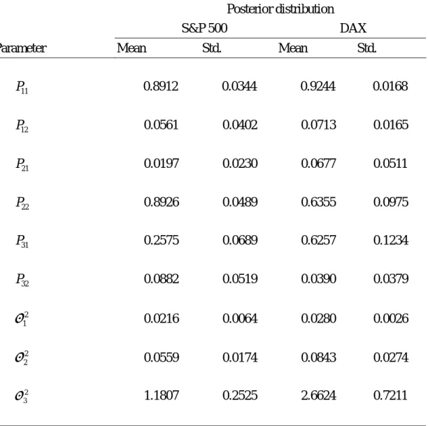
employ almost non-informative priors for all the models’ parameters. Table 1 presents
the marginal posterior distributions of the parameters that result from Gibbs-sampling
for the PCP deviations of S&P 500 and the DAX, respectively. At the end of each run
of Gibbs-sampling, we have a simulated set of
{
St, t =1,2...T}
and thus, of{
Sjt,t =1,2,...T, j=1,2,3}
, and . Figures 2(a), 2(b), 2(c) and Figures 3(a), 3(b), and 3(c) depict probabilities of low-, medium-, and high-variancestates for the PCP deviations of S&P 500 and the DAX, respectively, that result from
the Gibbs-sampling simulation.
3 , 2 , 1 , 2 = j j σ P%
Using the particular realizations of the states and the parameters for each run of
Gibbs-sampling, we can calculate σt2 for t=1,2,LT using equation (8). Thus, when all the iterations are over, we have 10,000 sets of realized variances
{
t t T}
T , 1,2,L ~2 = σ2 =
σ of PCP deviations. Figures 2(d) and 3(d) plot the average of
10,000 sets of σ~T2, which are our estimates of the variance of the S&P 500’s and the DAX’s PCP deviations. Tables 2 (a) and (b) present variance ratios for original daily
deviations from PCP for S&P 500 and DAX, respectively. Only the DAX displays
mean reversions at long horizons. The smallest p-value is 0.028 at 45 days lag.
Table 3 (a) and (b), in which variance ratios for standardized daily deviations
from PCP for S&P 500 and DAX are presented, respectively. The DAX also displays
mean reversion at long horizons and its smallest p-value is 0.028 at a lag of 40 days.
The evidence is weak that the standardized returns approach to estimating the VRs
8. Summary
Previous studies indicate that when market frictions are taken into account, the
deviations from PCP can fluctuate within a bounded interval without giving rise to
any arbitrage profit. This study presents a model of the option price mean reverting to
a function form of PCP. The variance ratio test is employed to examine whether the
deviations of PCP exhibit mean reversion. We make appropriate allowance for
heteroskedasticity when basing inference on the VR statistic by using the
Gibbs-sampling approach in the context of a three-state Markov switching model.
The empirical result shows that PCP deviations from the electronic
screen-traded DAX index options, which are calculated as if the dividends are
reinvested in the index, display mean reversion at long horizons. On the other hand,
those deviations from floor-traded S&P 500 index options, which do not correct for
Table 1:The estimated parameters from the Bayesian Gibbs-sampling approach to a three-state Markov-switching model of heteroskedasticity for S&P 500’s and DAX’s daily PCP deviations
Posterior distribution
S&P 500 DAX Parameter Mean Std. Mean Std.
P11 0.8912 0.0344 0.9244 0.0168 P12 0.0561 0.0402 0.0713 0.0165 P21 0.0197 0.0230 0.0677 0.0511 P22 0.8926 0.0489 0.6355 0.0975 P31 0.2575 0.0689 0.6257 0.1234 P32 0.0882 0.0519 0.0390 0.0379 σ12 0.0216 0.0064 0.0280 0.0026 σ22 0.0559 0.0174 0.0843 0.0274 2 1.1807 0.2525 2.6624 0.7211 3 σ
Table 2(a):Variance ratios for original daily deviations from PCP in S&P500
Lag(days) VR sampling distribution
(
VRr( )
k)
K VR(k) Mean Std Median p-value
2 1.4616 1.0343 0.0621 1.0340 1.0000 5 2.1525 1.0796 0.1266 1.0738 1.0000 10 1.1489 0.9957 0.0578 0.9950 0.9950 15 1.1816 0.9699 0.0922 0.9671 0.9854 20 1.2202 0.9536 0.1177 0.9491 0.9824 25 1.2907 0.9561 0.1385 0.9490 0.9864 30 1.3059 0.9564 0.1602 0.9467 0.9790 35 1.2527 0.9491 0.1812 0.9376 0.9440 40 1.1663 0.9425 0.2004 0.9288 0.8667 45 1.1181 0.9464 0.2172 0.9284 0.7957 50 1.0792 0.9496 0.2341 0.9290 0.7294
Note:1. The sampling distribution is based on Gibbs-sampling-augmented randomization.
2. The p-value is the frequency with which the simulated VR is smaller than the historical sample value, which is observed in the Gibbs-sampling-augmented randomization under the null hypothesis.
Table 2(b):Variance ratios for original daily deviations from PCP in DAX
Lag(days) VR sampling distribution
(
VRr( )
k)
K VR(k) Mean Std Median p-value
2 1.2283 1.0245 0.0648 1.0245 0.9991 5 1.5501 1.0438 0.1184 1.0401 0.9999 10 1.0528 0.9789 0.0471 0.9794 0.9456 15 1.0141 0.9520 0.0808 0.9529 0.7782 20 0.9131 0.9313 0.1043 0.9315 0.4293 25 0.8369 0.9294 0.1237 0.9257 0.2279 30 0.7666 0.9291 0.1450 0.9230 0.1305 35 0.6626 0.9216 0.1671 0.9131 0.0513 40 0.5893 0.9153 0.1859 0.9049 0.0282 45 0.5635 0.9174 0.2007 0.9050 0.0237 50 0.5484 0.9189 0.2158 0.9029 0.0254
Note:1. The sampling distribution is based on Gibbs-sampling-augmented randomization. 2. The p-value is the frequency with which the simulated VR is smaller than the historical
sample value, which is observed in the Gibbs-sampling-augmented randomization under the null hypothesis.
Table 3(a):Variance ratios for standardized daily deviations from PCP in S&P500
Lag(days) VR posterior distribution
(
VR*( )
k)
VR sampling distribution(
VRr*( )
k)
k Mean Std Median Mean Std Median p-value
2 1.5519 0.0209 1.5503 1.0001 0.0346 0.9998 1.0000 5 2.6193 0.0887 2.6043 0.9998 0.0758 0.9981 1.0000 10 1.3209 0.0387 1.3120 0.9982 0.0645 0.9984 1.0000 15 1.4444 0.0788 1.4244 0.9971 0.1047 0.9938 0.9996 20 1.5463 0.0975 1.5243 0.9963 0.1358 0.9911 0.9997 25 1.6176 0.0995 1.6000 0.9959 0.1619 0.9890 0.9995 30 1.6019 0.0992 1.5897 0.9958 0.1850 0.9862 0.9959 35 1.5043 0.0997 1.4955 0.9961 0.2063 0.9827 0.9811 40 1.3640 0.1008 1.3590 0.9966 0.2263 0.9803 0.9228 45 1.2431 0.1001 1.2410 0.9971 0.2449 0.9760 0.8256 50 1.1392 0.1031 1.1396 0.9975 0.2622 0.9726 0.7141
Note:1. The sampling distribution is based on Gibbs-sampling-augmented randomization 2. The p-value is the frequency with which the realizations of the Gibbs sampling of the
posterior distribution are smaller than the corresponding realization under the null hypothesis. 26
Table 3(b):Variance ratios for standardized daily deviations from PCP in DAX
Lag(days) VR posterior distribution
(
VR*( )
k)
VR sampling distribution(
VRr*( )
k)
k Mean Std Median Mean Std Median p-value
2 1.3804 0.0299 1.3852 1.0001 0.0343 1.0002 1.0000 5 2.0731 0.0830 2.0853 1.0001 0.0752 0.9979 1.0000 10 1.1008 0.0201 1.1017 0.9970 0.0642 0.9966 0.9388 15 0.9341 0.0389 0.9332 0.9963 0.1050 0.9931 0.2978 20 0.8265 0.0461 0.8252 0.9960 0.1367 0.9906 0.1166 25 0.8670 0.0449 0.8664 0.9963 0.1632 0.9876 0.2313 30 0.8349 0.0455 0.8347 0.9970 0.1868 0.9845 0.2062 35 0.7005 0.0483 0.7003 0.9976 0.2081 0.9801 0.0641 40 0.6078 0.0504 0.6068 0.9983 0.2281 0.9769 0.0277 45 0.6136 0.0526 0.6121 0.9991 0.2467 0.9728 0.0411 50 0.6213 0.0542 0.6196 1.0000 0.2645 0.9683 0.0580
Note:1. The sampling distribution is based on Gibbs-sampling-augmented randomization. 2. The p-value is the frequency with which the realizations of the Gibbs sampling of the
posterior distribution are smaller than the corresponding realization under the null hypothesis. 27
Figure 1(a):Daily PCP Deviations from S&P500
Figure 1(b):Daily PCP Deviations from DAX
Figure 2(a):Probability of a Low-variance State for S&P500’s PCP Deviations (Gibbs Sampling)
Figure 2(b):Probability of a Medium-variance State for S&P500’s PCP Deviations (Gibbs Sampling)
Figure 2(c):Probability of High-variance State for S&P500’s PCP Deviations (Gibbs Sampling)
Figure 2(d):Estimated Variance of S&P500’s PCP Deviations (Gibbs Sampling)
Figure 3(a):Probability of a Low-variance State for DAX’s PCP Deviations (Gibbs Sampling)
Figure 3(b):Probability of a Medium-variance State for DAX’s PCP Deviations (Gibbs Sampling)
Figure 3(c):Probability of a High-variance State for DAX’s PCP Deviations (Gibbs Sampling)
Figure 3(d):Estimated Variance of DAX’s PCP Deviations (Gibbs Sampling)
33
Reference
Albert, J. H. and Chib, S.(1993)“Bayes Inference via Gibbs Sampling of
Autoregressive Time Series Subject to Markov Mean and Variance Shifts”,
Journal of Business and Economic Statistics, 11, 1-15.
Brenner, M. and D. Galai (1986), “Implied Interest Rate”, Journal of Business, 59,
493-507.
Bühler, W. and A. Kempf, (1995), “DAX Index Futures:Mispricing and Arbitrage in
German Markets”, Journal of Futures Markets, 15, 833-59.
Casella, G. and E. I. George, (1993) “Explaining the Gibbs Sampler”, The American
Statistician 46(3), 167-174.
Chance, D. M.(1987)“Parity Tests of Index Options”, Advances in Futures and
Options Research, 2, 47-64.
Chib, S. and E. Greenberg, (1996) “Markov chain Monte Carlo simulation methods in
Econometrics”, Econometric Theory, 12, 409-431.
Cochrane, J. H.(1988)“How big is the random walk in GNP? ” Journal of Political
Economy, 96, 893-920.
Eleswarapu, V.R. and M.R. Reinganum, (1993), “The Seasonal Behavior of the
Liquidity Premium in Asset Pricing”, Journal of Financial Economics, 34, 373-86.
Evnine, J. and A. Rudd,(1985)“Index Options:The Early Exercise”, Journal of
Finance, 40, 743-55.
Gelfand, A. E. and A. F. M. Smith, (1990) “Sampling-Based Approaches to Calculating
Marginal Densities”, Journal of American Statistical Association, 85(410),
398-409.
Gould, J. P. and D. Galai,(1974)“Transaction Costs and Relationship Between Put and
34
Grünbichler, A., F. Longstaff, and E. S. Schwartz, (1994), “Electronic Screen Trading
and the Transmission of Information:An Empirical Examination”, Journal of
Financial Intermediation, 3, 166-87.
Hamilton, J. D.(1989), “A New Approach to the Economic Analysis of Nonstationary
Time Series and the Business Cycle”, Econometrica 57, 357-84.
___________(1990), “Analysis of Time Series Subject to Change in Regime”, Journal of Econometrics, 45, 39-70.
Harris, L.(1989)“The October 1987 S&P500 Stock-Futures Basis”, Journal of Finance, 43, 77-99.
Harvey, C. R. and R. E. Whaley (1992), “Dividends and S&P100 Index Option
Valuation”, Journal of Futures Markets, 12, 123-137.
Kamara, A. and T. W. Miller, (1995) “Daily and Intradaily Tests of European Put-Call
Parity”, Journal of Financial and Quantitative Analysis, 30, 519-39.
Kawaller, I.(1987)“A Note:Debunking the Myth of a Risk-Free Return”, Journal of
Futures Markets, 7, 327-31.
Kim, C. J. and Nelson, C. R. (1999), State-Space Models with Regime Switching:
Classical and Gibbs-sampling Approaches with Application, MIT press
Kim, M. J. , Nelson, C. R. and Startz, R.(1991)“Mean Reversion in Stock Prices?A
Reappraisal of the Empirical Evidence”, Review of Economic Studies 58, 515-28.
Kim, C. J. , Nelson, C. R. and Startz, R.(1998)“Testing for Mean Reversion in
Heteroskedasticity Data Based on Gibbs-Sampling-Augmented Randomization”,
Journal of Empirical Finance, 5, 131-54.
Kleidon, A.(1992)“Arbitrage, Nontrading and Stale Prices”, Journal of Business, 65,
483-507.
Klemkosky, R. C. and B. G. Resnick,(1979)“Put-Call Parity and Market Efficiency”,
35
___________,(1980)“An Ex Ante Analysis of Put-Call Parity”, Journal of Financial
Economics, 8, 363-78.
Lo, A. W. and A. C. MacKinlay,(1989)“The Size and Power of the Variance Ratio Test in Finite Samples:A Monte Carlo Investigation”, Journal of Econometrics, 40,
203-38.
Merton, R. C.(1973)“The Relationship between Put and Call Option Prices:
Comment”, Journal of Finance, 28, 183-84.
Miller, M. , J. Muthuswamy, and R. Whaley,(1994)“Predictability of S&P500 Index
Basis Changes:Arbitrage Induced or Statistical Illusion?” Journal of Finance, 49,
479-514.
Neal, R.(1996)“Direct Tests of Index Arbitrage Models”, Journal of Financial and
Quantitative Analysis, 31, 541-62.
Poterba, J. M. and L. H. Summers,(1988)“Mean reversion in Stock Prices:Evidence
and Implications”, Journal of Financial Economics, 22, 27-59.
Ronn, A. G. and E. I. Ronn,(1989)“The Box Spread Arbitrage Conditions:Theory,
Tests and Investment Strategies”, Review of Financial Studies, 2, 91-108.
Sofianos, G..(1993)“Index Arbitrage Profitability”, Journal of Derivatives, 1, 6-20.
Stoll, H. R.(1969)“The Relationship between Put and Call Option Prices”, Journal of