行動無線隨意網路之可適性拓撲控制

(1)

行動無線隨意網路之可適性拓撲控制

Adaptive Topology Control in Mobile Ad Hoc Networks

研究生: 鄭安凱

Student

:

An-Kai

Jeng

指導教授: 簡榮宏博士

Advisor: Rong-Hong Jan

國立交通大學

資訊工程學系

博士論文

A dissertation

Submitted to Department of Computer Science

College of Computer Science

National Chiao Tung University

in Partial

Fulfillment of the Requirements for the Degree of

Doctor of Philosophy

in computer Science

July 2007

(2)

國立交通大學

資訊工程學系

博士論文

行動無線隨意網路之可適性拓撲控制

Adaptive Topology Control in Mobile Ad Hoc Networks

研究生 : 鄭安凱

(3)

行動無隨意網路之可適性之撲控制

研究生: 鄭安凱指導教授 : 簡榮宏博士

國立交通大學資訊工程學系

摘要

在無線環境中，網路的效能會高度受到底層的拓撲所影響。而一個稀疏的拓撲具有減少多餘流量的特性，因此可提升網路擴增性。然而一個稀疏拓撲經常會犧牲許多重要的網路線段，這些線段有可能是型成要能源有效路由的必經路徑。因此，在拓撲的能源有效性和稀疏度之間存在了相互牽制的議題。在這篇論文中，我們將提出以幾合圖型為基礎的拓撲控制方法，這個方法可透過參數的設定達到在能源有效性和稀疏度之間調整的彈性，理論結果證明此方法可保證拓撲的連通性、平行性，和對稱性。更重要的是，每一個節點利用區域內所收集的資訊即可建構出所需的拓撲。為了解決節點的移動性，我們以前面的圖型方法為基礎，提出了一個可適性的拓撲控制協定，此協定具有在保有節點能源和改進整體耗能之間動態調整的能力。數據及摸擬結果提出，我們的方法可有效減少能源消耗，特別是對高度行動的網路有明顯的改進。

(4)

Adaptive Topology Control in Mobile Ad Hoc Networks

Student: An-Kai Jeng Advisor: Dr. Rong-Hong Jan

Department of Computer Science,

National Chiao Tung University

Abstract

The wireless ad hoc network is convenient to many applications, such as conferences, hospitals, battlefields, and etc. In these environments, the network performance heavily relies on the underlying topology. Especially, keeping the topology sparser enhances network scalability. However, a sparse topology may sacrifice some routes that consume less power. Therefore, a tradeoff is between the sparseness and the energy efficiency of the topology.

In this dissertation, we propose a geometric structure, named the r-neighborhood graph, to control the topology. The structure allows the flexibility to be adjusted between energy efficiency and node’s degree through a parameter r, 0 ≤ r ≤ 1. Theoretic results show that it can always result in a connected planar topology with symmetric edges. More importantly, the structure can be constructed in localized fashion using only 1-hop information.

To cope with node’s mobility, we investigate an adaptive protocol, based on a generalized version of the r-neighborhood graph. In this protocol, the parameter r can be adjusted distributively by each node according to the overall energy efficiency. To reduce the construction power, we further incorporate the protocol with a shrinking power mechanism for the topology maintenance. Simulation and numeric results show that the proposed approaches can significantly improve the energy consumption,

(5)

Acknowledgements

Special thank goes to my advisor Professor Rong-Hong Jan for his guidance in my dissertation work. Thank also to all member of Computer Network Lab for their assistance and kindly helping both in the research and the daily life during these years. Finally, I will dedicate this dissertation to my families for their love and support.

(6)

List of Tables

Table 2.1: The properties of the four main purely localizable structures………….. 13

Table 2.2: The properties of representative adjustable structures……….. 14

Table 4.1: The sufficient status of each variable……… 54

Table 6.1: The shrunken radius and power (n = 50)……….. 69

(9)

List of Figures

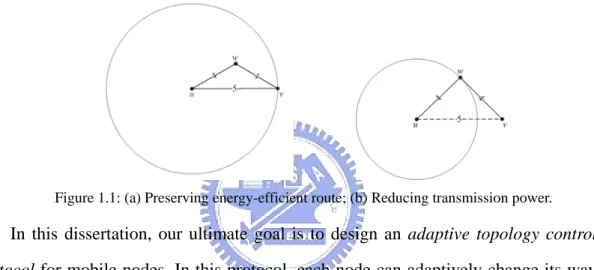
Figure 1.1: Preserving energy-efficient route vs. reducing transmission power …… 3

Figure 2.1: The RNG(V), GG(V), YGk(V), and UDel(V) ……… 10

Figure 2.2: The relations of pure localizable structures and their extensions ……… 12

Figure 3.1: The r-neighborhood region of nodes u and v ………... 18

Figure 3.2: The enclosed angles of two r-neighborhood regions ………... 25

Figure 3.3: The unbounded node degree without the assumption AS ……… 26

Figure 3.4: The r-neighbor region of nodes u and v, and in D2 and D3 ………. 27

Figure 3.5: The enclosed angles of two r-neighborhood regions in_NG*(_V)………… 28

r Figure 3.6: The worst-case instances V of n nodes in _NG*(_V)……… 33

r Figure 3.7: The r-neighborhood region vs. the (r, α)-neighborhood region ……….. 34

Figure 3.8: The(r, α)-relaying region vs. (r, α)-neighborhood region……… 37

Figure 3.9: The (r, α)-enclosed region……… 38

Figure 3.10: The (fr, fα)- neighborhood graph………. 39

Figure 4.1: The semicircle SC(u, v) and the circle χ(u, d)………... 43

Figure 4.2: the shrunk power λw and the enlarge power (r = 1, α = 2)……… 49

Figure 4.3: The statues of each variable over time intervals………... 56

Figure 5.1: The considerations of the self-configuration process……… 61 Figure 6.1: The upper bounds on the power stretch factor and maximum node degree

(10)

of NGr………...65

Figure 6.2: The topologies for 3 different levels of r. ……… 66 Figure 6.3: The power stretch factors the (r, α)-neighborhood graph……… 67

Figure 6.4: The maximum node degree of the (r, α)-neighborhood graph…………. 68

Figure 6.5: The shrinking power mechanism of variant r’s……… 69 Figure 6.6: The comparison of the overall energy-efficient……… 72

r

(11)

Chapter 1 Introduction

The continuing growing of techniques in mobile ad hoc network (MANETs) have led to many available applications in such as commercial, hospitals, military, search and rescue teams, education, etc. In MANETs, all transmissions are carried on wireless links without any wired connection, which enhances the conventional deployment of communicating environments. However, unlike a wired network, mobile devices are usually powered by limited energy supplies, where a continuing replacing or recharging could be hardly attainable. Hence, a substantial body of research has been devoted to improve the energy efficiency [34].

Due to the severe path loss in wireless links, the power required to transmit from one end to another will be exponentially grown by their distance. Thus, instead of a single long-distance transmission, relaying message through multiple hops with shorter distances usually consume less energy [24]. During the relaying process, each participating node has to consume energy to transmit or/and receive messages. Thus the total power required for a communication will be crucially influenced by the choice of relaying path. This motivates the recent research efforts on designing the energy-efficient communication protocols [35].

To compute the energy-efficient route, the global view of the network topology is required. However, the information is typically invisible to an individual node in

(12)

wireless environments. Thus, if without addition information, such as the position of destination, enormous control packets have to be flooded all over the entire network to find out the route. The incurred overhead will quickly drain out node’s energy.

In order to achieve the energy-efficient routing with less overhead, one promising way is by controlling the topology. Generally speaking, the basic idea is to keep the underlying topology as sparse as possible, while still preserve the energy-efficient route that consume less power for communications. A sparser topology can significantly mitigate the excessive flow flooded by nodes.

To reduce the communication overhead, one promising way is to control the underlying topology as sparse as possible to avoid excessive messages, while still preserve the energy-efficient route for any nodes pair. This is the so called

energy-efficient communication topology control problem. The topology control

problem in wireless ad hoc networks has been widely studied in recent years [3, 15, 18, 19, 20, 23, 29, 32]. Generally speaking, the core of this problem is to determine set of wireless links such that the composed topology is able to achieve certain goals [23]. These goals would be variant depending upon the circumstances and could be either qualitative features or quantitative objectives.

In general, the current effort on mobile topology control is mainly focused on reducing the transmission power required for each node to maintain the network connectivity. This objective is most appealing when the energy consumption of an individual node is crucial. However, to support an energy-efficient communication, the quality of routes preserved in the underlying topology is also important. Overall, the two goals are equally important in regard to deign an energy-efficient topology control: The former avoids exhausting individual node that in turn causes network partition and the later declines the per-packet energy consumption.

(13)

However, there is usually a tradeoff between the two desires: In order to constitute an energy-efficient route, a node may connect itself with a neighbor that is farther than the least requirement for connectivity. Contrarily, lowering down a node’ transmission power may instead increase the total relaying power. See the example in Figure 1.1 (a), the communicate power between u and v is 5, while the least power of

u to achieve connectivity is 3. In contrast, in Figure 1.1 (b), u’s transmission power is

minimal, while the total relaying power (4 + 4 = 8) is now worse.

Figure 1.1: (a) Preserving energy-efficient route; (b) Reducing transmission power.

In this dissertation, our ultimate goal is to design an adaptive topology control

protocol for mobile nodes. In this protocol, each node can adaptively change its way

to contribute to the overall energy efficiency: if a node has sufficient energy, it will aggressively participate in supporting the energy-efficient communication; and when the deposited energy downs to a relatively low level, the node will turn to conserve its own energy.

The main idea is based on a geometric structure, named the r-neighborhood

graph. The structure consists of several theoretic properties that can be exploited for

designing the mobile topology control with the adaptive goal. Most importantly, based on such structure, each node can decide its neighbors in a fully distributive and

(14)

extensions enable an elegant self-configuration process on each node

On the other hand, to keep the design clean and compatible with the IEEE 802.11 DCF, we let each node periodically announce its current position using beacon message. However, such maintenance power could be considerable, especially when the broadcasting range is large. For this reason, we incorporate the protocol with a

shrinking power mechanism. It can reduce the topology maintenance power

significantly.

Furthermore, our protocol can simultaneously achieve the following desirable features without additional control message.

1. Symmetric: A topology is symmetric if the presence of an edge uv implies that its inverse vu exists. If without the symmetricity, the implementations of many network primitives, such as ACK in link-layer, will be much complicated [21]. Our protocol ensures this property for any resulted topology.

2. Connected: Connectivity is unquestionably the most essential prerequisite in any communicable topology [23]. Two nodes u and v are strongly connected if there is a directed path from u to v and vice versa. A directed topology is strongly connected if all pairs of nodes are strongly connected. If the links are symmetric, we should aim at the connectivity of an undirected topology.

3. Sparse: Numerous distributed and localized routing protocols are based on flooding [13]; however this may burden networks with unavoidable redundant messages. Thus, keeping a sparse topology, consisting of linear number of links [15], would be an ingenious way to shrink the expenditure from network operations. 4. Bounded Maximum node degree: For some nodes with overly-large degrees, the network flows will concentrate on them and rapidly draw out their energy. Besides, a larger node degree means tighter dependency among nodes, which is not expected

(15)

when wireless nodes move frequently. Therefore, the maximum node degree over a topology should be bounded from above by some constant.

5. Planar: A graph is planar if it has no crossed links inside. It is helpful for many geometric problems: The shortest path (least energy unicast route) can be quickly found in linear time when the underlying topology is planar [12]; Besides, in many position-based routing algorithms, the successful delivery can be guaranteed only if the underlying topology is a planar [2, 11].

In addition, in wireless ad hoc networks, due to the absence of a central arbitrator and the limited sensing range, a centralized approach for controlling the topology is rarely attainable [3, 30]. Therefore, a variety of distributed approaches were proposed[17,19,29]. A distributed protocol passes messages hop-by-hop. This however may cause considerable overhead through the entire network. So, a localized approach is more preferred. According to the definition given by Stojmenovic and Lin [27], a localized topology control approach allows each node to determine its neighbors using only constant hop information. However, in some localized approaches [15, 16, 18, 27], the operations should recursively depend upon the computed status or partial results from nearby nodes, which may hurt their practicability. Therefore, in the following we define a new type of mythology for more practicability.

DEFINITION 1.1: An algorithm L is purely localized if it is localized and all operations

depend upon only the information inherent1 in nodes, available before any execution of L.

A purely localized topology control algorithm is more useful to large scale and high mobility environments, since the operation of a node is completely isolated from any

1

The node’s position and id are usually assumed to be inherited in nodes. See Chapter 2 for more explanation.

(16)

execution of other nodes. Further, we say that a structure is purely localizable if we can construct it by a purely localized algorithm. One of our goals is to investigate a purely localizable structure so that all desired features mentioned above can achieve.

The rest of this dissertation is organized as follows. Chapter 2 specifies the network model and formally describes the problem under study. In Chapter 3, we review and summarize the related works. The main geometric structures, components, and their theoretical results are presented in Chapter 4. In Chapter 5, we suggest a localized algorithm for stationery nodes and a shrinking power mechanism to constitute the skeleton of the desired protocol. In Chapter 6, we present the theoretic definition, properties, and algorithms of the self-configured process in mobile environment. Extensive simulation and numeric studies are conduced in Chapter 7. Finally, concluding remarks and some worth directions for the further research are given in the last Chapter. Detailed derivations are given in Appendix.

(17)

Chapter 2 Background and Related Works

In this chapter, the network model studied in this dissertation will be formally described. Then, we will review some related works in the literature. According to the assumption of node mobility, existing works for stationary and mobile nodes will be discussed, respectively, in Chapter 2.2 and Chapter 2.3.

2.1 Network Model

The wireless ad hoc network concerned in this paper consists of a set V of n wireless nodes distributed on a deployment region ℵ, which is a subset of the

two-dimension plane ℜ2

. We assume that each node is equipped with an omnidirectional antenna and can change its transmission range by adjusting the transmitting power at any level. The maximum transmission ranges are equal among all nodes. In other words, we can normalize the maximum transmission ranges of all nodes to be 1 for simplicity. In addition, each node u can obtain its location Loc(u) through a lower-power GPS or some other ways [14], and an unique id(u) is also available to each node u.

This network can be modeled as a unit disk graph, UDG(V). In this graph, an edge uv exists if and only if the Euclidean distance between u and v, denoted as ||uv||, is at most 1.

(18)

The least power required to transmit immediately between u and v is modeled as

p(u, v) = ||uv||α, where α is typically taken on a value between 2 and 4, depending on

the attenuation strength of the communication environment [5]. To measure the power efficiency of a topology, Li et al. [15] defined a well-formed measure, named power

stretch factor. We reintroduce it as below.

Let π(u, v) = v0v1…vh-1vh be a unicast path connecting nodes u and v, where v0 = u and

vh = v. The total transmission power consumed by path π(u, v) is defined as

∑

= − = h i i i v v p v u p 1 1, ) ( )) , ( (π .

Let be the least-energy path connecting u and v in graph G(V). Given a

controlled topology S(V) of UDG(V), tthe power stretch factor of S(V) with respect to

UDG(V)is defined as,

) , ( * ) (V u v G π

(

)

(

( , )

)

) , ( max )) ( ( _* ) ( * ) ( , _p _u _v v u p V S V UDG V S V v u π π ρ ∈ = .

This factor indicates the worst ratio of the least energy required to relay on S(V) in compared to that of a uncontrolled topology for all possible communication pairs. Clearly, a smaller ratio is preferable. On the other hand, the maximum node degree of the topology S(V) is defined as

)) ( ( max )) ( ( max S V d G V d _u V u∈ = ,

where du(S(V)) is the degree of node u in S(V).

In addition, the following symbols will be used throughout this article. z D(u, d): the closed disk centered at Loc(u) with radius d.

z C(u, d): the circled centered at Loc(u) with radius d. z N_u(G(V)): the set of neighbor of u in a graph G(V).

(19)

2.2 Stationery Topology Control

In the field of topology control for stationary nodes, a majority of researches were conducted by designing the proximate graph. A proximate graph is a geometric structure in which each node determines its neighbors based on the positions of nodes in its province. In other words, a topology approach based on such structure can be carried out in a fully distributed and localized way. A number of instances can be found in the literature [15, 16, 18, 26]. These works are diverse in their sparseness and the energy efficiency of preserved routes. We discuss the most well-know structures below. Most of them or their extensions are purely localizable:

 The constrained Relative Neighborhood Graph [28], denoted by RNG(V), has an edge uv if and only if ||uv|| ≤ 1 and the intersection of two open disks1

centered at

u, v with radius ||uv|| contains no node w ∈V, see Figure 2.1 (a),

 The constrained Gabriel Graph [6], denoted by GG(V), has an edge uv if and only if ||uv||≤ 1 and the open disk using ||uv|| as diameter contains no node w ∈V, see Figure 2.1 (b).

 The constrained Yao Graph [33] with a parameter k ≥ 6, denoted by YGk(V) is

constructed as follows. For each node u, define k equal cones by k equal-separated rays originated at u. At each cone, a directed edge uv exists, if ||uv|| ≤ 1 and the cone contains no vertex w ∈V such that ||uw|| < ||uv||. Ties are broken arbitrarily. YGk(V) is denoted as the underlying undirected graph of

) (V

YGk , see Figure 2.1 (c).

 A Delaunay Triangulation, denoted by Del(V), is a triangulation of V in which the interior of the circumcircle of each Δuvw contains no node w ∈ V. The unit

1

An open disk centered at point x with radius d is the collection of points with distance less than d from Loc(x).

(20)

Delaunay Triangulation, denoted by UDel(V), has all edges of Del(V) except

those longer than 1 [8, 18], see Figure 2.1 (d).

(a) (b)

(c)

(d) Figure 2.1: (a) RNG(V) (b) GG(V) (c) YGk(V), k = 8 (d) UDel(V).

Let us discuss the properties of these structures and their extensions. We say a objective f(.) of a structure S(V) is bounded if there is a constant C such that f(S(V)) ≤

C, for any set V of n nodes. Li et al. [15] showed that dmax(RNG(V)) is unbounded if

there is a node u ∈ V having an unbounded number of neighbors adjacent to u at exactly the same distance in the underlying UDG(V). To overcome this problem, Wattenhofer and Zollinger [32] proposed an algorithm to find a structure, denoted by

XTC(V). They showed that that XTC(V) is a subgraph of RNG(V) and the dmax(XTC(V))

(21)

the same distance in V, XTC(V) is identical to RNG(V) [24]. Their results infer the following theorem.

THEOREM 2.1: Given a set V of nodes on ℜ2, if there is no node having two or more

neighbors at exactly the same distance, then dmax(RNG(V)) ≤ 6.

We denote the condition in Theorem 2.1 as assumption AS. That is,

AS : There is no node in V having two or more neighbors at exactly the same distance.

This theorem reveals that even RNG(V) has no constant bound on its node degree, it is still useful since the distances of nodes in real world are rarely exactly the same. The constrained Gabriel Graph GG(V) has the least power stretch factor 1, in comparison with the unbounded power stretch factor n – 1 of RNG(V) [15]. However, dmax(GG(V))

could be as large as n – 1. An extended structure, Enclosure graph [16, 14, 24], denoted by EG(V) is generalized from GG(V). It can always result in a subgraph of

GG(V) [16]. Even so, its maximum node degree is still unbounded [20, 24].

To overcome the tradeoff between the maximum node degree and the power stretch factor, an adjustable structure, having the flexibility to be adjusted between the two objectives, becomes more attractive. YGk(V)is an adjustable structure. It can be

adjusted through a parameter k such that for any given k, the maximum out-degree is at most k, and the power stretch factor is at most 1

(

1−

(

2sinπ/k

)

α

)

[15]. We say an objective f(.) of an adjustable structure Sk(V) with parameter k is partially bounded if

there is at least one k0 such that is bounded. According this definition, the

maximum out-degree and power stretch factor of )) ( ( 0 V S f _k ) (V

YGk are partially bounded

since for some ranges of k, k and 1

(

1−

(

2sinπ/k

)

α

)

are constants. However, the asymmetric edges of YGk(V) may lead to large in-degrees even when k is very small

[15]. So, can be neither bounded nor partially bounded. To improve

this, an extension of )) ( ( max YG V d _k ) (V

(22)

limit the maximum node degree in (k +1)2 – 1 and result symmetric edges. Unfortunately, in this structure the neighbors of some node should be recursively determined by one another so that it can not be purely localizable. The unit Delaunay triangulation UDel(V) has bounded power stretch factor. However, neither Del(V) nor

UDel(V) can be computed locally. So, Li et al. [18] suggested a localized version of

the Delaunay graph, denoted by LDel(h)(V), where h means that each node uses at most k-hop information. The power stretch factor of LDel(k)(V) is bounded for all k ≥ 1. Even so, its maximum node degree is not bounded for any h.

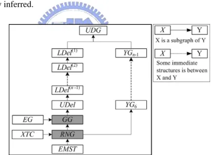
The relations among these structures were studied in several papers [7, 10, 16, 22, 24, 33]. We summarize them on Figure 2.2, where EMST(V) is the Euclidean minimum spanning tree of UDG(V). With these relations, their connectivity can planarity can be easily inferred.

Figure 2.2: The relations of the pure localizable structures and their extensions.

Regarding the connectivity: we know that EMST(V) is connected if UDG(V) is itself a connected component of V. Therefore, when UDG(V) is connected, all graph containing EMST(V) are connected. That is, RNG(V), GG(V), EG(V), UDel(V),

(23)

LDe(k)l(V), YGk(V) are all connected. The connectivity of XTC(X) was proven by

different way [24].

Regarding the planarity: LDel(k)(V) is planar for any k ≥ 2 [18]. Therefore, all subgraphs of LDel(2)(V) are planar. That is, UDel(V), GG(V), EG(V), RNG(V), XTC(V),

EMST(V) are all planar. On the contrary, YGk(V), and LDe(1)l(V) can not avoid

producing the crossed link, so they are not planar [15, 18]. Table 2.1 summarizes above discussion.

From above table, we can see that no presented structure can bound or even partially bound the two objectives. Besides to the best of our knowledge, no other structure can be purely localizable and achieve this goal. Therefore, we will propose the first purely localizable structure, named r-Neighborhood Graph, to fill this gap. This structure is adjustable and can always result in a connected planar with symmetric edges. In addition, we can show that our structure is a generation of both

GG(V) and RNG(V).

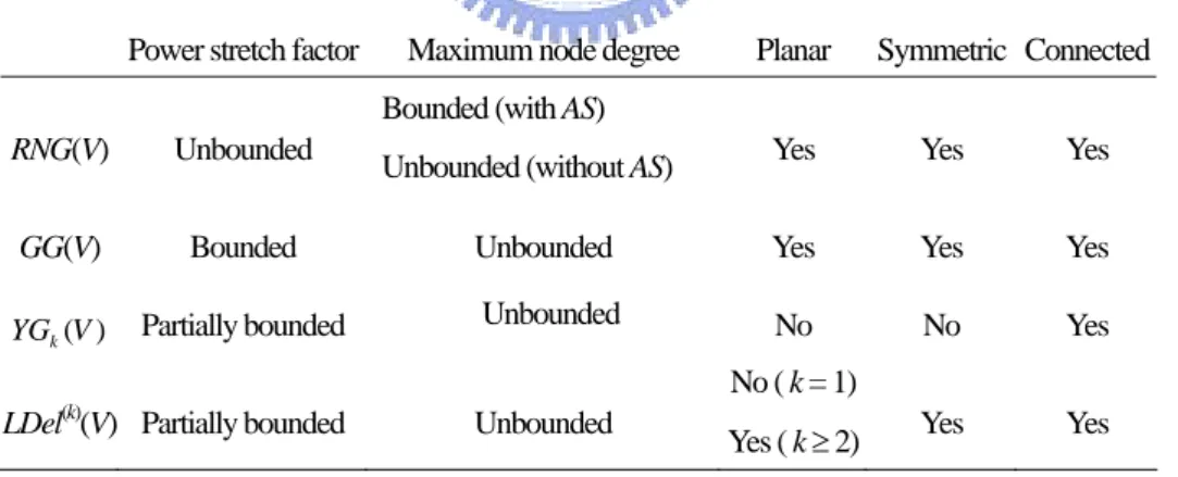
Table 2.1: The properties of the four main purely localizable structures. Power stretch factor Maximum node degree Planar Symmetric Connected

RNG(V) Unbounded

Bounded (with AS)

Unbounded (without AS) Yes Yes Yes

GG(V) Bounded Unbounded Yes Yes Yes

) (V

YGk Partially bounded

Unbounded _{No No Yes}

LDel(k)(V) Partially bounded Unbounded

No ( k = 1)

Yes ( k ≥ 2) Yes Yes

Apart from the purely localizable structures, several composite methods, based on combining two or more existent structures, were investigated in the last few years [17, 19, 25, 31]. Conceptually, the main idea is to use the virtue of one structure to

(24)

patch up the fault in the other structures. For examples, the ordered Yao structure,

denoted as OrdYao(V) [1], is a variation of . It has the partially bounded

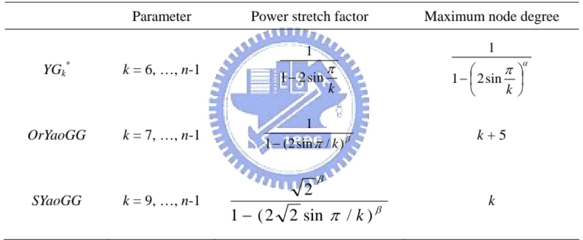
maximum node degree and length stretch factor. However, the planarity can not be guaranteed. Therefore, Wang and Li [19, 31] applied OrdYao(V) onto LDel(2)(V) to avoid the crossed edges produced by OrdYao(V); Song et al. [25] improves it by applying the OrdYao(V) on GG(V), using only one-hop information. Their Result are summary in Table 2.2. However, the construction of OrdYao(Y) requires exchanging the computed status as well as partial results between nodes. Consequently, none of them is purely localized or purely localizable.

) (

*

V YG_k

Table 2.2: The properties ofrepresentative adjustable structures.

Parameter Power stretch factor Maximum node degree

YGk* k = 6, …, n-1 k π sin 2 1 1 − π⎟α ⎠ ⎞ ⎜ ⎝ ⎛ − k sin 2 1 1 OrYaoGG k = 7, …, n-1 ₁ ₍₂_sin_π_/ ₎β 1 k − k + 5 SYaoGG k = 9, …, n-1 _β β π / ) sin 2 2 ( 1 2 k − k

2.3 Mobile Topology Control Protocols

Distributed protocols for proximate graphs can be also found in the literature [34]. However, existent results are all applied to stationary network only. There is no approach explicitly designed for mobile nodes based on such structure. The reason is probably that the construction depends on node positions, so that even a slight change in nodes placement could trigger a reconstruction process to handle the broken link or

(25)

deteriorated link quality.

There are relatively fewer works considering nodes mobility. The LINT (and its extension LILT) is perhaps the first topology control protocol explicitly designed for mobile network [36, 37]. In this protocol, each node continually adjusts its transmission power such that the number of covered neighbors is within a lower and high threshold. Accordingly, the energy can be saved by declining the high threshold, and the network connectivity can be achieved by uplifting the low threshold. It however has no guarantee on connectivity if the low threshold is underestimated. To improve that, Blough et al [38] proposed a similar approach, named the K-NEIGH. The protocol connects each node with its k-closest neighbors and removes all asymmetric links, where k is a predefined parameter. The most interesting result is that if n nodes are uniformly distributed at random and k is taken as Θ(logn), then the connectivity can be held with high probability. These protocols are called the

neighbor-based approach, since a node’s construction relays on the ability of ordering

or measuring distances of nodes in its province [34]. The direction-based approach is another stem. It uses the angles among nodes for the construction. An example is the Cone Based Topology Control (CBTC) [39]. The basic idea is to let each node transmits with the minimum power that covers at least one neighbor in every cone of an angle ρ centered at it. The authors show that ρ ≤ 2π/3 is a sufficient condition to ensure connectivity. Li et al. [40] proposed a reconfiguration procedure to deal with node mobility by detecting changing events from received beacons.

The most important features of these protocols are that their constructions are based on either nodes distance or nodes directions. Compared with the proximate graph, both the neighbor-based and direction-based approaches can be more accommodating to nodes movement. The reason is that the changing on nodes

(26)

distances or directions will be relatively small with respect to nodes positions. Therefore, by using either of the two less precise information, a fewer number of topology reconstruction will be required when nodes move.

Even thought our protocols are based on a proximate graph. We will show that such disadvantage can be easily mitigated in an elegant way. In addition, Compared with K-NEIGH, LINT (LILT) and CBTC, our protocol guarantees the network connectivity in any stabilized status, without any assumption on nodes distribution, or parameter setting. Furthermore, both CBTC and K-NEIGH attend symmetricity by exchanging linking status among nodes. This will incur additional control overhead. Our protocol ensures that any established link is inherently bidirectional.

(27)

Chapter 3 Graphic Structures

In this chapter, we will introduce a new adjustable structure, called the

r-neighbor graph. It can be adjusted between the maximum node degree and power

stretch factor through the parameter r. The structure can also produce connected planar with symmetric edges. However, its maximum node degree will be unbounded in certain cases. To comprehend the theoretic property, we will then propose an enhanced version, called the extended r-neighborhood graph to deal with the special circumstance.

To apply the proposed structure to our mobile protocol, extensive investigations on the r-neighborhood graph will be given. First of all, we define a generalized structure, called the (r, α)-neighborhood graph. The generalization can gain better quantitative results. Next, an equivalent structure, called the (r, α)-Enclosed graph will be given. Its diverse representation enables the design of a shrinking power mechanism in Chapter 4. Then, we further generalized the structure such that each node having its own r, named the (fr, α)-neighborhood Graph. This graph provides

essential properties for the self-configuration process in Chapter 6.

3.1 r-Neighborhood Graph

(28)

ℜ2

. It will be used to compose our structure.

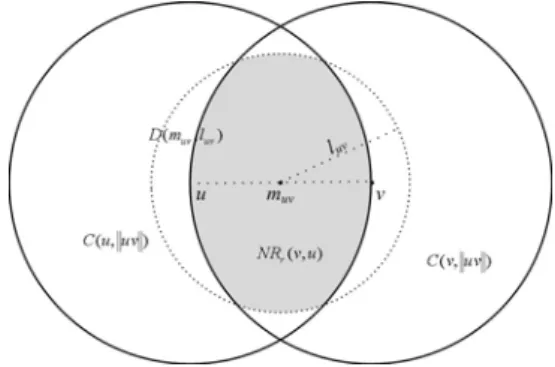
DEFINITION 3.1: Given a nodes pair (u, v) on ℵ, the r-neighborhood region of (u, v),

denoted as NRr(u, v), is defined as:

) , ( ) , ( ) , ( ) , ( _uv _uv r u v D u uv D v uv D m l NR = ∩ ∩ ,

where muv is the middle point on uv, luv = (||uv||/2)(1 + 2r2)1/2, and 0 ≤ r ≤ 1.

Figure 3.1: The r-neighborhood region of nodes u and v.

When no confused, we use m and l instead of muv and luv respectively. In Figure 3.1,

the shaded region intersected by the three open disks sketches an example of the

r-neighborhood region. This region is obviously equivalent to the following point set:

} , , | ) ( { ) , (u v Loc x 2 ux uv vx uv mx l NR_r = ∈ℜ < < < (3.1)

For any node w located on NRr(u, v), this region limits the power consumed by path

uwv. This property is shown in Lemma 3.1 and derived in Appendix.

LEMMA 3.1: Given two nodes u and v on ℵ, for any node w such that Loc(w) ∈ NRr(u,

v), p(uwv) < ||uv||α(2 + rα), for all α ≥ 2.

This lemma explains why we call such plane a neighborhood region: For any node w located in the region NRr(u, v), it should be an alternative neighbor for u with respect

to v, in the sense that the power required for relaying from u to v through w is no greater than 1 + rα times of the immediate transmission. Based on this region, we structure is defined below.

(29)

DEFINITION 3.2: Given a set V of nodes on ℵ, the r-neighborhood graph of V,

denoted as NGr(V), has of an edge uv if and only if ||uv|| ≤ 1 and NRr(u, v) contains no

node w ∈ V, where 0 ≤ r ≤ 1.

By Definition 3.2, if edge uv is not in UDG(V) or a node w is inside NRr(u, v), there is

no direct link connecting u and v in NGr(V), which mean that all transmissions

between u and v should be relied through some other node(s) in NGr(V). Now, we

explore the desired properties in our structure. Before this, we shall discussion the following relations.

LEMMA 3.2: For any set V of nodes on ℵ, RNG(V) ⊆ NGr(V) ⊆ GG(V), for all 0≤ r≤1.

Proof. Consider the open disk D(m, ||uv||/2), defining GG(V). Suppose uv ∈ NGr(V),

the region NRr(u, v) has no node inside. Since D(m, ||uv||/2) is obviously a subregion

of NRr(u, v), for any 0 ≤ r ≤ 1, there is also no node in D(m, ||uv||/2). Therefore,

according to the definition of GG(V), we get uv ∈ GG(V). On the other hand, consider the two open disks D(u, ||uv||) and D(v, ||uv||), defining RNG(V). Suppose uv ∈

RNG(V), no node is inside the intersection of D(u, ||uv||) and D(v, ||uv||), which

obviously covers the region NRr(u, v), for any 0 ≤ r ≤ 1. Therefore, no node can be

inside NRr(u, v) and we get uv ∈ NGr(V). □

Specifically, as r = 0, NR0(u, v) ≡ D(m, ||uv||/2), which is the disk defining GG(V). On

the contrary, as r = 1, NR1(u, v) ≡ D(m, ||uv||), which is the disk defining RNG(V).

Therefore, GG(V) ≡ NG0(V) and RNG(V) ≡ NG1(V). So, we can conclude the

following theorem.

THEOREM 3.1: The r-neighborhood graph is a generalized structure of both the

restricted Gabriel graph and the restricted relative neighborhood graph.

Since a subgraph of a planar graph is always planar, and a supergraph of a connected graph is always connected, with the planarity of GG(V) and connectivity of RNG(V),

(30)

we can infer the following two theorems.

THEOREM 3.2: For any set V of nodes on ℵ, NGr(V) is planar, for all 0 ≤ r ≤ 1.

THEOREM 3.3: For any set V of nodes on ℵ, if the underlying UDG(V) is connected,

NGr(V) is connected, for all 0 ≤ r ≤ 1.

Now we consider the energy efficiency and node degree of NGr(V). We will

show that the upper bound of ρ(NGr(V)) is increased by r and contrarily the upper

bound of dmax(NGr(V)) is decreased by r. In other words, the r-neighborhoodgraph is

adjustable to the two objectives through the parameter r. With these results, we can further show that the power stretch factor and maximum node degree are partially bounded in our structure. Before these, a property proposed by Li et al.[15] shall be mentioned first. It can be used to simplify our proof.

LEMMA 3.3 [15]: Given a subgraph G’(V) ⊆ UDG(V) and a constant C, ρ(G’(V)) ≤ C

if and onlyiffor any edge uv in G(V), there is a path π(u, v) in G’(V) such that

α uv C v u p_G_'₍_V₎( , )≤ .

This lemma indicates that to derive an upper bound for ρ(NGr(V)), it is sufficient to

the consider only those nodes pairs having direct links in UDG(V). So, we aim to derive a strictly decreasing function F(r), such that for any uv in UDG(V), a path

) , ( vu

π is in NGr(V) such thatp

(

π( vu, )

)

≤ F(r)||uv||α. To achieve this, we investigate

an algorithm EXPANSION with an input of any two nodes (u, v) and outputs subgraph S

of NGr(V) related to (u, v). Let P(S) be the total transmission power of edges in S. i.e.

P(S) = ∑st∈Sp(s, t). We can show that there is some path in S connecting (u, v) and P(S)

≤ F(r)||uv||α.

In this algorithm, S’ is a set of nodes pairs, in which an edge st in NGr(V) can be a part

of S only if its two ends (s, t) are in S’ as described at step 3. So, to determine S, we have discuss the S’ first. Initially, S’ contains only (u, v). Then, it will be recursively

(31)

expanded as follows: for each (s, t) in S’, if a node w is in NRr(s, t) and not considered

before, replace (s, t) with (s, w) and (w, t); if a node w is in NRr(s, t) but considered

before, replace (s, t) with (s, w); Otherwise, keep (s, t) unchanged. We use the set Q to record the considered nodes.

ALGORITHM EXPANSION

Input: A nodes pair (u, v) in V

Output: A subgraph S and a positive value P.

Step 1: S = {}, S’ ={(u, v)}, Q = {u, v}, P = ||uv||α;

Step 2: When some node pair (s, t) is in S such that a node w ∈ NRr(s, t)

S’ = S’ – (s, t); If w ∉ Q then S’ = S’ ∪ (s, w) ∪ (w, t); Q = Q ∪{w}; P = P + (||st||r)α; Otherwise, S’ = S’ ∪ (s, w); Step 3: S = {xy ∈ NGr(V) | (x, y) ∈ S’};

Step 4: Stop and output E and P.

When some (s, t) is in S’ such that a node w ∈ NRr(s, t), no matter w is

considered or not, by (4.1), the replaced nodes pair(s) must be shorter than ||st||. i.e. ||sw|| < ||st|| and ||wt|| < ||st||. Thus after finite iterations, each node pair in S’ can be replaced by another node pair with shortest distance. So, the algorithm is terminable. Now we show that (u, v) is connected by some path in the subgraph S when termination.

(32)

LEMMA 3.4: Given any set V of node on ℵ, for any two nodes u and v in V, if edge uv

is in UDG(V) and UDG(V) is connected, there is some path in S connecting (u, v).

Proof: Since Q includes u and v, we can prove this lemma by showing that all nodes

in the Q are connected in S. For each expansion of S’, we define a dummy graph S” in which an edge st exists if and only if (s, t) is in S’ (Note that any edge in S” is not necessarily in either UDG(V) or NGr(V)). First, we show that at any iteration, all

considered nodes in Q are connected by S”. Initially, Q is connected by S”, since S’ = {(u, v)} and Q ={u, v}. We assume for induction that all nodes in Q are connected by

S” at k-th iteration. Then, we show that it is true for the next iteration. At k+1-th

iteration, if there is no pair in S’ satisfies the entrance condition of step 2, the claim is correct, since Q and S” are unchanged; Otherwise, a node pair (s, t) ∈ S’ is expended. In this case, if the chosen w ∉ Q, w is connected with all nodes in Q via dummy edges

sw and wt; otherwise, w ∈ Q, which implies all nodes in Q are still connected by S” as

the previous iteration. As described above, the distance of any expended nodes pair is no longer than the previous one. So, if uv is in UDG(V), all edges in S” are also in

UDG(V). Then, as the algorithm processes to step 3, no nodes can be in the r-neighborhood region of any nodes pair in S’. With these two facts, all dummy edges

in S” are also in NGr(V) when termination. So S is equivalent to the last S”.

Consequently, if UDG(V) is connected, by Theorem 4.4, all nodes in the last Q are

connected S. □

Then we derive a strictly decreasing function F(r) using the value P in this algorithm. LEMMA 3.4: Given any set V of n nodes on ℵ, for any two nodes u and v in V,

α uv r F S P( )≤ ( ) and F(r)=1+(n−2)rα

for all 0 ≤ r ≤ 1 and α ≥ 2.

(33)

Initially, S’ = {(u,v)}. We can get P(S’) = ||uv||α = P. Then at the first iteration, if no node w is in NRr(u, v), the claim remains true since neither P nor S is changed;

Otherwise, a node w is in NRr(u, v). Besides, any chosen w can not be in Q, since no

nodes except u and v are in Q so far. So, uv is replaced by vw and wv. By Lemma 4.1,

P(vw)+P(wu) ≤ P(uv)(1+rα) = P + (||uv||r)α. Consequently the new P remains a upper bound of P(S’) . We assume for induction that P(S’) ≤ P at k-th iteration. Then we prove the claim is true at the next iteration. If the entrance condition of step 2 is not satisfied or the chosen w ∉ Q, it can be proved by the same reasons as in the first iteration. Otherwise, assume (s, t) is taken, st is replaced by only sw. By (4.1), P(vw) ≤

P(uv), which implies that the unchanged P is still an upper bound of P(S’). Besides,

(4.1) further implies that all distance of two nodes in E are no greater than ||uv||. So, another upper bound P’ can be get by replacing P = P + (||st||r)α by P’ = P’ + (||uv||r)α. Moreover, we can observe that the situation that as a w is chosen from some NGr(s, t)

is not in Q never happens over n – 2 times, since in this case the size of Q must be increased 1. Consequently, P(S’) ≤ P ≤ P’ ≤ P(uv) + P(uv)rα(n – 2) . Finally, we get

F(r) = (1+rα)(n – 2). □

With lemmas 3.3, 3.4 and 3.5, we can conclude the following theorem. THEOREM 3.4: ForanysetVofnnodesonℜ,forall0≤r ≤ 1 and α ≥ 2,

) ( ) 2 ( 1 )) ( (NG_r V ≤ +rα n− =F r ρ .

Although this bound is related to the node size n so that ρ (NGr(V)) can not be

bounded, it can still be constant when r is 0 or some sufficiently small. i.e. ρ (NGr(V))

is bounded in some range of r. So, we can make the following conclusion.

COROLLARY 3.1: The power stretch factor of the r-neighborhood graph is partially

bounded.

Consider the maximum node degree of the r-neighborhood graph. Since NGr(V)

(34)

that of RNG(V). In Chapter 2, we know that dmax(RNG(V)) is not always bounded in

any case of V. Thus, dmax(NGr(V)) is also unbounded. Fortunately, Theorem 2.1

indicates that dmax(RNG(V)) is bounded in most cases of V, where AS is assumed.

Therefore, in the following theorem, we analyze the maximum node degree of the

r-neighborhood graph under assumption AS.

THEOREM 3.5: For any set V of nodes on ℵ with assumption AS, for all 0 ≤ r ≤ 1,

⎡

/sin ( /2)

⎤

)) ( ( 1 max NG V r d _r ≤ π − .

Proof. To prove this statement, it is sufficient to show that in , there are no adjacent edges enclosing an angle less than 2sin-1(r/2). Assume for contradiction that two edges uv and uw in enclose an angle θ < 2sin-1(r/2) at node u, where w,

v ∈ V. Without a loss of generality, we assume that ||uw|| < ||uv||. With assumption AS,

all nodes are placed on different positions. i.e. Loc(x) ≠ Loc(y), for any two nodes x, y ∈ V; Consider the length of vw: If ∠uwv is obtuse, it is clear that ||vw|| < ||uv|| (note that ||vw|| can not be equal to ||uv||, since Loc(u) ≠ Loc(w)), see Figure 3.2 (b); Otherwise, if ∠uwv is not obtuse, ||vw|| is less ||vw’||, where ||uw’|| = ||uv||, see Figure 3.2 (a). By the law of cosine, we have

) (V NG_r ) (V NG_r θ cos ' 2 ' '2 uw 2 uv 2 uw uv vw = + − θ cos 2 2uv 2 − uv 2 =

( )

(

2sin /2

)

cos 2 2uv 2− uv 2 −1 r < (3.2)

Letθ'=2sin−1

(

r/2

)

, we get sin

(

θ'/2

)

=r/2 . Then one of the corresponding

right-angled triangles is as shown in Figure 4.2 (c). In this case, .

Thus we can get that

2 / ) 2 ( ' cosθ = −r2

( )

/

(

)/2

)

sin 2 −1 r 2 =θ'=cos− (2−r2 . Consequently, (3.2) =2uv 2 −2uv 2cos

(

cos−

(

2−r2

)

/2

)

(

)

(

2 /2

)

2 2uv 2− uv 2 −r2 = 2 2 r uv = (3.3)

(35)

{

uvr uv

}

uv

vw <max , = (3.4)

Consider the length of um: if ∠uwm is obtuse, ||wm|| < ||uv||/2 see Figure 3.2 (b); Otherwise, ||mw|| is less ||mw’||, see Figure 3.2 (b). By the law of cosine, we have

θ cos ' ' 2 ' ' ' 2 uw 2 um 2 uw um mw = + − . θ cos 4 / 2 2 2 uv uv uv + − <

(

)

(

2 /2

)

4 / 5uv 2 − uv 2 −r2 < = uv 2

(

1+2r2

)

/4

)

(3.6)

Similarly, we have for any case of ∠uwm

{

uv r uv

}

l

mw <max 1+2 2 /2, /2 = . (3.6)

By (3.4), (3.6) and the assumption of ||uw|| < ||uv||, w is included in the set of points specified in (3.1). Therefore, P(w) ∈ NRr(u, v). It however contradicts the assumption

that uv is in NGr(V). Thus we conclude this theorem. □

(a) (b) (c)

Figure 3.2: (a) ∠uwv and ∠uwm are not obtuse; (b) ∠uwv and ∠uwm are obtuse; (c) a right-angled triangle with angleθ=2sin−( )r/2 .

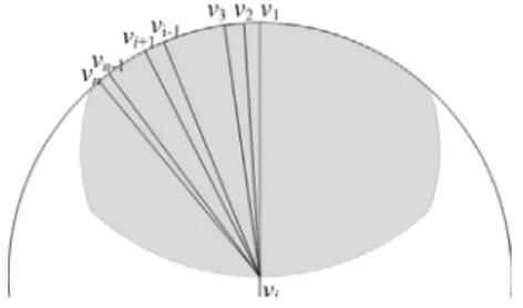
However, for those instances of V without AS, Theorem 3.5 can not hold anymore. See the instance in Figure 3.3, all nodes except vi are placed on the outlier

of NRr(vi, v1). This will result n – 1 neighbors adjacent to vi in NGr(V). So, in the next

section, we propose an extended version the r-neighborhood graph. As the readers will see, the extended structure has the partially bounded maximum node degree for

(36)

all cases of V and inherits almost all desired features in NGr(V).

Figure 3.3: dmax(NGr(V)) is not bounded if assumption AS does not hold.

3.2 Extended r-Neighborhood Graph

In this section, an extended structure of the r-neighborhood graph is given. The

main goal is to avoid the unbounded maximum node degree in NGr(V). In this

extension, assumption AS is not required anymore. Instead, a unique identifier id(u) is available to each node u in V. The structure is defined as follows.

DEFINITION 3.3: Given a set V of nodes ℵ, the extended r-neighborhood graph of V,

denoted as , has an edge uv if and only if ||uv|| ≤ 1 and there exists no node w ∈ V satisfying one of the following three conditions:

) ( * V NG_r D1: Loc(w)∈NRr(u,v); D2: Loc(w)∈D(muv,luv)∩C(v, uv)andid(u)>id(w); D3: Loc(w)∈D(muv,luv)∩C(u, uv)andid(v)>id(w).

Without D2 and D3, is clearly equivalent to the original r-neighborhood

graph. In conditions D2 and D3, the two sub-regions of D(muv, luv) intersected by C(v,

||uv||) and C(u, ||uv||) are, as depicted in Figure 3.4, the solid left arc and right arc along the outlier of NRr(u, v), respectively. When a node w is located in these two arcs,

the existence of edge uv should be further determined by their identifiers. )

(

*

V NG_r

(37)

Hereafter, we say that a node w ∈ V blocks an edge uv in UDG(V) if and only if w satisfies one of the three conditions in Definition 3.3.

Figure 3.4: The r-neighbor region of nodes u and v, and the two intersections defined in D2 and D3.

In , an edge uv of UDG(V) will not only be blocked by some node w

in , but may also be blocked when either D2 or D3 happens. Therefore,

constitutes a subgraph of NGr(V), which means that the maximum node

degree of is no worse than its original version. In the following theorem,

we show that the upper bound of in Theorem 3.5 remains correct in

, and the correctness is for any case of V, not subject to assumption AS. ) ( * V NG_r ) , v u ) ( * V NG_r )) ( * V r ( NR_r ( * V NG_r ( max NG ) )) ( ( max NG V d _r d

THEOREM 3.6: For any set V of nodes on ℵ, for all 0 ≤ r ≤ 1,

⎥ ⎥ ⎤ ⎢ ⎢ ⎡ ≤ ₋ ) 2 / ( sin )) ( ( * ₁ max r V NG d _r π .

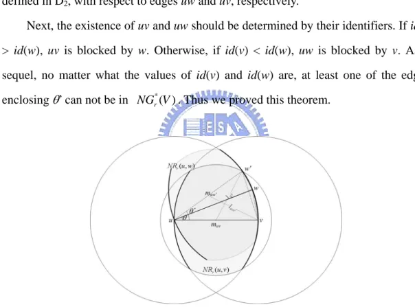
Proof. Using the same argument as Theorem 3.5, we assume for contradiction that

two edges uv and uw in enclose an angle at node u.

Without loss of generality, we assume that ) ( * V NG_r θ'<2sin−1(r/2) uv uw ≤ . If uw < uv , the argument

of Theorem 3.5 has proved the contradiction. Consider uw = uv : Let be a

point crossed by C(u, ||uv||) and the outlier of D(muv, luv), as shown in Figure 3.5. The

two edges and uv enclose an angle

'

w

u

(38)

(

)

uv uw w m uv uw _uv ' ' 2 / ' ' cos 2 2 2 − + = θ

(

)

uv uv l uv uv uv 2 2 2 2 2 / − + = =1+r2/2

Then one corresponding right-angle triangulation is as Figure 3.2 (c). In this case,

(

'/2

)

/2

sinθ =r . Thus, we can get that θ <θ'=2sin−1(r/2). Since uw = uv , both

Loc(w) and Loc(v) are on C(u, ||uv||). The fact that θ <θ' further limits Loc(w) on the arc intersected by D(muv, luv). Similarly, Loc(v) is limited on the arc intersected by

D(muw, luw) for the same reason. Therefore, Loc(w) and Loc(v) are on the regions

defined in D2, with respect to edges uw and uv, respectively.

Next, the existence of uv and uw should be determined by their identifiers. If id(v) > id(w), uv is blocked by w. Otherwise, if id(v) < id(w), uw is blocked by v. As a sequel, no matter what the values of id(v) and id(w) are, at least one of the edges enclosing θ’ can not be in NG_r*(V). Thus we proved this theorem. □

Figure 3.5: If θ < 2sin-1

(r/2) and ||uw|| = ||uv||, either uw or uv can not be in NG*r(V)

From Theorem 3.6, we can see that is constant when r is sufficiently

large. Therefore, there has some setting of r such that is bounded by

some constant, for any set V of n nodes. So, we reach the following conclusion. )) ( ( * max NG V d _r )) ( ( * max NG V d _r

(39)

COROLLARY 3.2: The maximum node degree of the extended r-neighborhood graph

is partially bounded.

In the rest part, we show that inherits all desired properties achieved

by NGr(V), except the generality for RNG(V). The fact that

confirms the planarity of , since NGr(V) is planar for any r. Moreover, when

r = 0, the two arcs defined in D2 and D3 are empty. Thus whether an edge is in

is solely depending on D1, which means that .

Therefore, remains a general structure of GG(V).

) ( * V NG_r ) ( ) ( * V NG V NG_r ⊆ _r ) ( ) ( 0 V GG V NG ≡ ≡ ) ( * V NG_r ) ( * V NG_r NG₀*(V) ) ( * V NG_r

However, as shown Theorem 3.6, some adjacent edges having the same length in

RNG(V) would be avoided in . Thus RNG(V) is not always a subgraph of

. This means that is not essentially equivalent to RNG(V). Even

more, could be a subgraph of RNG(V). Therefore, is no longer a

general structure of RNG(V). ) ( * V NG_r ) ( * 1 V ) ( * V NG_r NG NG ) ( * 1 V ( ) * V NG_r

About the connectivity, because RNG(V) is not always a subgraph of ,

we cannot ensure the connectivity of directly from that of RNG(V).

Therefore, we apply an entirely different logic to prove this property. The idea is based on comparing the lexicography orders of nodes pairs. This idea has been successfully used to prove the connectivity of XTC(V) [32], another subgraph of

RNG(V). ) ( * V NG_r ) ( * V NG_r

We define a three-field tuple (||uv||, id(u), id(v)) for each nodes pair (u, v). The lexicographic order of (u, v) is smaller than that of another nodes pair (s, t) if one of the following three cases happens: 1) ||uv|| <||st||; 2) ||uv|| =||st|| and id(u) < id(s); 3) ||uv|| =||st|| , id(u) = id(s) and id(v) < id(t). Now, we prove the connectivity of

in Theorem 3.7. ) ( * V NG_r

(40)

) (

*

V

NG_r is connected, for all 0 ≤ r ≤ 1.

Proof. Suppose UDG(V) is connected. Let U(V) be the set of unconnected nodes pairs

in . We assume for contradiction that some nodes pairs in are not

connected. i.e., U(V) is not empty. Let (u, v) be the node pair with smallest lexicographic order in U(V).

) (

*

V

NG_r NG_r*(V)

Assume that edge uv is not in UDG(V), i.e. ||uv|| > 1. Since UDG(V) is connected, there must be some path longer than one hop connecting u and v. Let π(u, v) be such path in UDG(V). Since ||uv|| > 1, the lengths of each edge on π(u, v) is less than ||uv||.

When this path is mapped to , there is some nodes pairs on π(u, v)

unconnected in . Thus some unconnected node pair on π(u, v) has length

shorter than ||uv||, which however contradicts that (u, v) has the smallest lexicographic order in U(V). Therefore, edge uv must be in UDG(V).

) ( * V NG_r ) ( * V NG_r

Since edge uv is in UDG(V) and not in , there must be some node w satisfying

one of the three conditions in Definition 3.3. Besides, either (u, w) or (w, v) is in U(V), otherwise (u, v) can be connected by path uwv. We consider the three cases:

) (

*

V NG_r

1) If D1 happens, Loc(w) ∈ NRr(u, v). So, we has ||uw|| < ||uv|| and ||wv|| < ||uv||, which

means that the lexicographic orders of (u, w) and (w, v) are less than that of (u, v). 2) If D2 happens, we have ||wv|| = ||uv|| and id(u) > id(w), which means that the

lexicographic order of (w, v) is less than that of (u, v);

3) If D3 happens, we have ||uw|| = ||uv|| and id(v) > id(w), which means that the

lexicographic order of (u, w) is less than that of (u, v).

Therefore, we cannot find any nodes pair in U(V) having the smallest lexicographic order. In other words, U(V) is empty, which however is a contradiction. Thus, we

proved this. □

(41)

not inNG*_r(V). Therefore, ρ(NG_r*(V)) is no better or even worse than ρ(NG_r(V)).

Even so, the upper bound of can be as good as that proved in Theorem

3.4; we briefly explain this: All arguments in Theorem 3.4 are not related to the two additional conditions D2 and D3, except those referred from Lemma 3.1. Whatever D1,

D2 or D3 happens, ||uw|| ≤ ||uv||, ||vw|| = ||uv|| and ||mv|| < l, which means that all

inequalities in the proof of Lemma 3.1 are unchanged. Consequently, Theorem 3.4 is still correct, even if all conditions of Definition 3.3 are considered. So,

is also partially bounded.

)) rα ( (NG_r* V ρ 1+ )) ( (NG_r* V ρ )) V

Below, we show that the bound in Theorem 3.4 is not only correct,

but also asymptotically tight to the worst possible value of . In other

words, it is very hard to find another upper bound of better than ours.

We apply the same argument as that used to verify the tightness of the length stretch factor [3] and the power stretch factor [15] of RNG(V)

) 2 (n− ( (NG_r* ρ )) (V (NG_r* ρ

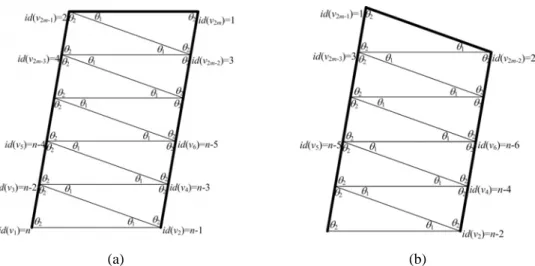
THEOREM 3.8: For any n ≥ 2 and 0 ≤ r ≤ 1, there is a set V of n nodes such that ε α ₋ ₋ + = 1 ( 2) sup r n n V ρ(NG_r*(V))> , for any sufficient smallε >0.

Proof. Let θ1 = 2sin–1(r/2) – 2λ and θ2 = π/2 – sin–1(r/2) + λ, where λ > 0. We

construct a set V = {v1, v2, …,v2m–1,v2m,…, vn}of n nodes, where n ≥ 2 is even and m =

n/2 , as follows:

, for i = 2, 3,…, 2m – 1; 1) v₁v₂ ≤1 and v_iv_i₊₁ = v₁v₂

2) ∠vivi+1vi+2 = θ1, for i = 1, 2,…, 2m – 2;

3) ∠vi+2vivi+1 = ∠vivi+2vi+1 = θ2, for i = 1, 2,…, 2m – 2;

4) id(vi) = n – i + 1, for i = 1, 2,…, n;

One corresponding UDG(V) is as shown in Figure 3.6. For i = 1, 2,…, 2m – 2, since ∠vivi+1vi+2 = θ1 < 2sin-1(r/2) and vivi+1 = vi+1vi+2 , by the argument in Theorem 7, we

(42)

get . That is, is in the regions with respect to edge vivi+1, defined in D2. Moreover, . Thus, edge vivi+1 is

not in . Then, the remaining edges are exactly a path (spanning tree)

v1v3v5…v2m–3v2m–1 v2mv2m–2…v6v4v2 of V, connecting all nodes, as the bold links in

Figure 3.6 (a). Therefore, we can get that ) , ( ) , ( ) ( 1 1 1 2 ∈ + ∩ + + + i i vivi vivi i D v v C m l v P ) ( * V NG_r ) (v_i₊₂ P ( )> i id v ) ( v_i₊₂ id

(

)

∑

− = + − + =2 2 1 2 1 2 2 ) m i m m i iv v v v rα α α 2 1 * ) ( ( , *_V NG v v p r π 0 →

As λ , , which implies that θ₁→2sin−1(r/2) v_iv_i₊₂ →r v_iv_i₊₂ =r v₁v₂ , according to (3.3). Consequently, as λ→0, we get that

∑

− = + − + 2 2 1 2 1 2 2 m i m m i iv v v v rα α α

∑

− = + →2 2 2 2 1 2 1 h i v v v v rα α α

(

( 2) 1

)

2 1 − + = α α r n v v

On the other than, since v₁v₂ ≤1, we get p

(

π_UDG* ₍_V₎(u,v)

)

= uvα . Therefore, as

0 →

λ , _NG_(V₎(UDG(V))→1+rα(n−2). That is,

r ρ ε ρ _> ₊ α ₋ ₋ = ( ( )) 1 ( 2) sup_|_V_| _n NG_r* V r n ,

for any sufficient ε >0. For any odd n ≥2, the result can be obtained by applying the

same argument to the instance as shown in Figure 3.6 (b). So, we proved this it. □

Actually, an equivalent structure of , without a original version like

NGr(V), was mentioned in our previous paper

) ( * V NG_r 2

[9]. In that preliminary work, however only qualitative results were given. To prove the quantitative results, we separate

NGr(V) from in this paper, because NGr(V) has a clearer form in definition

that can be used to highlight the main tricky in our derivations. Besides, all qualitative results in [9] are re-evaluated here using different arguments.

) ( * V r NG 2

The term “r-neighborhood graph” in [9], is not refereed to the original version in Definition 3, but the extended version in Definition 4. In this paper, we reuse the same term to name the original version and

(43)

(a) (b)

Figure 4.6: A worst-case instance V of n nodes in _NG*(_V): (a) n is even; (b) n is odd.

r

3.3 (r,

α

)-Neighborhood Graph

In [7], we showed that for any point x∈ NRr(u, v), ||ux||α + ||xv||α < ||uv||α (1 + rα).

This result combined with Definition 3.2 indicates that if an edge uv of UDG(V) is not in NGr(V), there must be a node w located in NGr(u, v), such that p(u, w) + p(w, v) <

p(u, v)(1 + rα). In other words, for any uv ∈ UDG(V), if there is no node w such that p(u, w) + p(w, v) < p(u, v)(1 + rα), then uv ∈ NGr(V). The upper bound of the power

stretch factor in Theorem 3.4 is then an inductive consequence of this fact. This argument implies the following lemma,

LEMMA 3.6: For any graph S(V), if it contains an edge uv, whenever there is no other

node w such that p(u, w) + p(w, v) < p(u, v)(1 + rα), then ρ(S(V)) ≤1 + rα(n – 2). According to this lemma, a structure that has the same upper bound on the power stretch factor of NGr(V) is defined as follows.

DEFINITION 3.3: Given two nodes u and v on ℵ, a parameter r, 0 ≤ r ≤ 1, and a

constant α≥ 2, the (r, α)-neighborhood region, is defined by

{

| , , ( , ) ( , ) ( , )(1 )

}

) , ( α α r v u p v x p x u p uv vx uv ux x v u NR_r = ∈ℵ < < + < + .

(44)

DEFINITION 3.5: Given a set V of nodes on ℵ, the (r, α)-neighborhood graph, denote

as , has an edge uv if and only if ||uv|| ≤ 1 and there is no other node w

located in .

) (V

NG_rα

NR_rα( vu, )

Figure 3.7: NRr(u, v) vs. NRrα(u, v).

Their relationships are as follows. We can see that is actually a general

structure of NGr(V). Notably, it achieves the same upper bound on the power stretch

using equal or less edges.

) (V

NGr

α

PROPERTY 3.1: For any two nodes u and v on ℵ, 0 ≤ r ≤ 1, and α ≥ 2

(i)NGr (V)⊆NGr(V);

α

(ii)NG_r2(V)≡NG_r(V).

Proof: Consider an edge . By definition, there is no node w such that

, which implies that uv ∈ NGr(V).

) (V NG uv r α ∈ ) 1 )( +rα , ( ) , ( ) , (u w p w v p u v p + <

Consider an edge . There is no nodes w such that ||mw|| < (||uv|| /

2)(1 + 2r2)1/2. Consider a point x. From simple derivation, we get

) (V NG uv∈ _r 2 2 2 2 2 2 \ xm uv vx ux + = + .

Combining these two facts, ux2+ vx2 < uv 2(1+rα). So, uv NGr (V).

α

∈

行動無線隨意網路之可適性拓撲控制

行動無線隨意網路之可適性拓撲控制

Adaptive Topology Control in Mobile Ad Hoc Networks

研 究 生: 鄭安凱

Student

:

An-Kai

Jeng

指導教授: 簡榮宏 博士

Advisor: Rong-Hong Jan

國 立 交 通 大 學

資 訊 工 程 學 系

博 士 論 文

A dissertation

Submitted to Department of Computer Science

College of Computer Science

National Chiao Tung University

in Partial

Fulfillment of the Requirements for the Degree of

Doctor of Philosophy

in computer Science

July 2007

國 立 交 通 大 學

資 訊 工 程 學 系

博 士 論 文

行動無線隨意網路之可適性拓撲控制

Adaptive Topology Control in Mobile Ad Hoc Networks

研 究 生 : 鄭安凱

行動無隨意網路之可適性之撲控制

研 究 生: 鄭安凱 指導教授 : 簡榮宏 博士

國立交通大學 資訊工程學系

摘要

Adaptive Topology Control in Mobile Ad Hoc Networks

Student: An-Kai Jeng Advisor: Dr. Rong-Hong Jan

Department of Computer Science,

National Chiao Tung University

Abstract

Acknowledgements

Contents

List of Tables

List of Figures

Chapter 1

Introduction

Chapter 2

Background and Related Works

2.1 Network Model

∑

(

)

(

)

2.2 Stationery Topology Control

(

(

)

)

(

(

)

)

2.3 Mobile Topology Control Protocols

Chapter 3

Graphic Structures

3.1 r-Neighborhood Graph

(

)

⎡

⎤

( )

(

)

(

)

(

)

( )

(

)

(

(

研究生: 鄭安凱

指導教授: 簡榮宏博士

國立交通大學

資訊工程學系

博士論文

國立交通大學

資訊工程學系

博士論文

研究生 : 鄭安凱

研究生: 鄭安凱指導教授 : 簡榮宏博士

國立交通大學資訊工程學系