國
立
交
通
大
學
物理研究所
碩
士
論
文
Lennard-Jones 流 體之瞬 間正則模 頻譜內 遷移邊界 的 多重 碎形分 析
Multifractal analysis for mobility edge in the instantaneous normal mode
spectra of Lennard-Jones fluids
研 究 生:施益慎
指導教授:吳天鳴 教授
Lennard-Jones 流體之瞬間正則模頻譜內遷移邊界的多重碎形分析
學生:施益慎 指導教授:吳天鳴
國立交通大學物理研究所
摘要
在本論文中,探討在 Lennard-Jones 位能交互作用下的流體內瞬間正則模之局域至 非局域轉變,即系統由局域模態到擴張模態的轉變。而在瞬間正則模頻譜中,分別存在 有實頻與虛頻瞬間正則模之局域至非局域遷移邊界。我們利用瞬間正則模在遷移邊界上 表現出多重碎形的特性,即奇異頻譜及振動幅度的機率密度函數在遷移邊界上不隨系統 大小改變, 就此特性進行推估遷移邊界所在位置的頻率。但實頻遷移邊界在計算上仍 然有因系統效應難以克服之問題,無法準確計算出遷移邊界,因此本文主要探討虛頻瞬 間正則模遷移邊界。我們的結果證實奇異頻譜幾乎與安德森模型在臨界亂度及在一簡單 短程斥力流體內正則模之遷移邊界具有良好的一致性。在不同的熱力學狀態下,正則模 遷移邊界也仍然具有一致相同的多重碎形特性,且在振動幅度的機率密度函數上的最大 值具有不隨系統大小改變的特性。Multifractal analysis for mobility edge in the instantaneous normal mode
spectra of Lennard-Jones fluids
Student:Yi –Shen Shih Adviser:Ten-Ming Wu
Institute of Physics
National Chiao-Tung University
Abstract
In this thesis, we have investigated the localization-delocalization transitions (LDTs) of the instantaneous normal modes (INMs) in simple fluids with Lennard-Jones (LJ) potential. The LDT is the transition of the instantaneous vibrations in the system from the localized to extended states. The INM spectrum of a simple fluid consists of the real- and imaginary-frequency branches, corresponding to the positive and negative eigenvalues. The multifractal properties of the INMs at a mobility edge (ME) show that the singularity spectrum (SSP) and the probability density function (PDF) of vibrational amplitudes are invariant with the system size. Therefore, we use these properties to locate the ME in an INM frequency spectrum. Since the multifractal analysis for the ME in the real-frequency branch still has the formidable system size effect, we are not able to locate the ME precisely. So, we only consider the ME in the imaginary-frequency branch. Our results indicate that the singularity spectrum of the multifractal INMs almost agrees with that of the Anderson Model (AM) at the critical disorder and that of the INMs at the ME of the short-range truncated Lennard-Jones fluid. Also, for the LJ fluids at the thermodynamic states that we have simulated, the SSP of the multifractal INMs still has the same agreement. This agreement is a numerical evidence for the universality of the multifractals at the LDT. Besides this, within numerical errors, the location of the maximum in the PDF of vibrational amplitudes is also evidenced to be invariant with the system size.
致謝
感謝我的家人對於我就讀碩士班的兩年期間,給我不只是精神上及經濟上的支持, 更要感謝我的指導教授吳天鳴教授和所上教授在課業上及做人處事上的諄諄教誨,讓我 學習到一個研究生應該有的行為跟表現,我深感獲益良多,最後還要感謝交大的同學、 學長及學弟,還有一群一起到新竹讀研究所的大學同學,讓我在這兩年的期間中有歡笑 也有淚水,因為有你們的陪伴才能有今天小小的成就。List of tables and figures ... 2
1. Introduction ... 4
2.Theory ... 6
2.1 Instantaneous normal modes of simple fluids ... 6
2.2 INMs at Mobility Edge ... 9
2.3 Multifractal Analysis ... 10
2.3.1 Fractal Dimension and Singularity Spectrum ... 12
2.3.2 Box-size scaling and System-size scaling ... 15
2.3.3Probability Density Function of Vibrational Amplitudes ... 16
2.4Multifractality of INMs at ME ... 17
2.4.1 Determination of mobility edge by MFA ... 18
3.Model and Numerical method ... 19
3.1The Lennard-Jones potential ... 19
3.2The Monte Carlo method ... 22
3.3 The JADAMILU method ... 24
4.Results... 26
4.1 Box-size scaling and system-size scaling for different thermodynamics
states ... 26
4.2 Singularity spectrum... 39
4.3Probabilty density function of vibrational amplitudes ... 42
5.Conclusions ... 53
Appendix A ... 55
A.1 Derivation for Legendre Transform of SSP from the Mass Exponents 55
Bibliography ... 57
List of tables and figures
Table3.1: Coefficient A and B in different cutoff distance………..20 Table3.2:Five different thermodynamic states of LJ fluids with different cutoff distance,
reduced density, reduced temperature, Nc and equilibrium MCsteps. ………20
Fig(3.1) The truncated Lennard-Jones (TLJ) potential (the dashed line) , Lennard-Jones
potential with two different cutoff distances =2.5 and =3.5 (the red solid and block solid line, respectively) and full Lennard-Jones potentail. ………..21
Fig(3.2-a) The radial distribution functions of LJ fluids for three different cutoff distances
under same reduced density and reduced temperature. ………22
Fig(3.2-b) The radial distribution functions of LJ fluids for different reduced density under
same cutoff distance, and reduced temperature. ………..22
Fig(3.2-c) The radial distribution functions of LJ fluids for different reduced temperature
under same cutoff distance, reduced density. ………...23
Table 4.1: The cube of the length is calculates by L= . ………..26
Table.(4.2) The ME at different thermodynamic states ………...28 Table.(4.3) The position of the singularity strength (q=0) under box-size scaling and
system-size scaling. ………..29
Fig.(4.1-a) At thermodynamic state , the box-size scaling
of the singularity spectrum of the INMs LJ simple fluids at a ME. ……….30
Fig.(4.1-b) At thermodynamic state , the system-size
scaling of the singularity spectrum of the INMs LJ simple fluids at a ME. ………….31
Fig.(4.2-a) At thermodynamic state , the box-size scaling
of the singularity spectrum of the INMs LJ simple fluids at a ME. ………..32
Fig.(4.2-b) At thermodynamic state , the system-size scaling
of the singularity spectrum of the INMs LJ simple fluids at a ME. ………..33
Fig.(4.3-a) At thermodynamic state , the box-size scaling of
the singularity spectrum of the INMs LJ simple fluids at a ME. ………..34
Fig.(4.3-b) At thermodynamic state , the system-size scaling of
the singularity spectrum of the INMs LJ simple fluids at a ME. ………..35
Fig.(4.4-a) At thermodynamic state , the box-size scaling of
the singularity spectrum of the INMs LJ simple fluids at a ME. ………..36
Fig.(4.4-b) At thermodynamic state , the system-size scaling of
Fig.(4.5-a) At thermodynamic state , the box-size scaling
of the singularity spectrum of the INMs LJ simple fluids at a ME. ………..38
Fig.(4.5-b) At thermodynamic state , the system-size
scaling of the singularity spectrum of the INMs LJ simple fluids at a ME. ………….39
Fig(4.6-a) The system-size scaling of the singularity spectrum of the INMs LJ simple
fluids at a ME under different thermodynamic states. ……….40
Fig(4.6-b) The box-size scaling of the singularity spectrum of the INMs LJ simple
fluids at a ME under different thermodynamic states. ……….41
Fig.(4.7-a) At thermodynamic state , the probability
density function of vibrational amplitudes change with different simulated system size for INMs LJ fluids at . . ………..43
Fig.(4.7-b) At thermodynamic state , the singularity
spectrum of the INMs LJ simple fluids at a ME. ………..44
Fig.(4.8-a) At thermodynamic state ,the probability density
function of vibrational amplitudes change with different simulated system size for INMs LJ simple fluids at . . ………45
Fig.(4.8-b) At thermodynamic state , the singularity
spectrum of the INMs LJ fluids at a ME. ………..46
Fig.(4.9-a) At thermodynamic state , the probability density
function of vibrational amplitudes change with different simulated system size for INMs LJ fluids at . . ………...47
Fig.(4.9-b) At thermodynamic state , the singularity spectrum
of the INMs LJ fluids at a ME. ………..48
Fig.(4.10-a) At thermodynamic state , the probability density
function of vibrational amplitudes change with different simulated system size for INMs LJ fluids at . . ………...49
Fig.(4.10-b) At thermodynamic state , the singularity spectrum
of the INMs LJ fluids at a ME. ………..50
Fig.(4.11-a) At thermodynamic state , the probability
density function of vibrational amplitudes change with different simulated system size for LJ fluids INMs at . . ………..51
Fig.(4.11-b) At thermodynamic state , the singularity
Chapter1
1. Introduction
The localization-delocalization transition (LDT) induced by disorder has been known for many years. No matter for Anderson Model (AM) or other physical systems related with waves [1,2,3,4,5,6,7], the researches on this subject are more active. Thanks for the recent advance in computers and algorithms, the AM has been calculated at even larger sizes so that the investigations for the multifractality at the LDT are also considerably progressed. The LDT also happens to vibrational excitations, the waves of atomic motions, in disordered media. [8,9,10,11]. The studies of vibrational excitations have the benefit to avoid the complicated many body problems. Vibrational modes are classified into extended modes and localized modes: The extended modes are in perfect lattices and the localized modes causes by impurities and defects in the disordered lattices. Such as amorphous materials, the disorder in atomic structures makes the systems performed not like a lattice anymore. The vibrational modes at low frequencies are generally extended and the high-frequency modes are localized. Therefore, the LDT occurs at some vibrational frequency; this special point is called to be a mobility edge (ME). The ME provides an alternative universality for investigating. Recently, localization of ultrasound is observed in a three-dimensional elastic network of aluminum beads and the localized ultrasounds show strong multifractality [4,12].
In this thesis, we are interested in the LDT in the instantaneous-normal-mode (INM) spectrum of simple fluids [13]. We want to confirm that the ME of the INMs has the universal properties for fluids with different ranges in the pair potential and at different thermodynamic states. Therefore, we calculate the eigenmodes of the Hessian matrices at the instantaneous configurations. The fluid configurations are not necessary located at the local minima of
the multifractal analysis and the probability density function of vibrational amplitudes, we identify the location of the negative-eigenvalue ME in the INM spectrum. But, these two methods for the ME in the real-frequency branch have the formidable system size effect.
Our results agree with the AM at the critical disorder and the INM spectrum of a simple fluid with TLJ potential. This agreement indicates that the MEs in the INM spectra of simple fluids with the LJ potential and at different thermodynamic states still have the universality. In the future, how to remove the formidable system size effect on the location of the ME in the real-frequency branch and solving the crystallization problem of the simple fluids at high densities or low temperatures are still considerable issues. Moreover, generalizations of the multifractal analysis to other physical systems are also the future works.
Chapter2
2.Theory
2.1 Instantaneous normal modes of simple fluids
We consider a fluid of N particles with equal mass. The total potential energy V(R) of the fluid at a configuration R, which is a 3N-dimensional vector indicating the particle positions, is a sum of the pair potential for all particle pairs
=
In a short-time scale, a harmonic approximation can be applied for V(R) [14], and by expanding V(R) to the second order of particle displacement about R0, V(R) is approximated
as
V(R)=V(R0)-F(R0)‧(R-R0)+ (R- R0)‧K(R0)‧(R- R0), (2.1.1)
where F(R0) denotes 3N-dimensional force vector. Since R0 may not be a configuration at
local minimum of V(R), F(R0) is generally non-zero. K(R0) is the 3N3N Hessian matrix
composed of 3X3 blocks, which are functions of relative displacements of particle pairs. With
U=R-R0, the displacement from R0 the harmonic potential in Eq.(2.1.1), the equations of
the motion are
=U-K-1.F,
this leads to the equation of motion
=-K(R0). .
A configuration of the fluid system can be specified as a point on the potential energy
surface (PES) of V(R) in the 3N-dimensional space. The evolution of the system can be
described by the motion of the point on the PES, which is composed of many mountains, valleys and saddle points. The eigenmodes of the Hessian matrix at a configuration are referred as the instantaneous normal modes (INMs) of the system. The eigenvalues of the INMs are associated with the curvatures of the PES, where a positive eigenvalue corresponds to a valley along the normal mode degree of freedom, while a negative one represents the curvature at a mountain top or on a shoulder along another normal mode degree of freedom. The square roots of the eigenvalues characterize the frequencies of the INMs. It is justified that only the negative-eigenvalue INMs specified as “true unstable modes” contribute to the self-diffusion coefficient of the fluid system [15]. Here, the “true unstable modes” mean that the steepest descent paths along the eigenvector direction of an unstable mode and along the reversed direction on the PES will not lead to the same local minimum of V(R) in the 3N-dimensional space. And, the number of local minimum does not lose in this process.
For a fluid with the pair potential , the elements of Hessian matrix K(R0), which are
the second derivatives of V(R) with respect to the particle displacements, are expressed as = , = t(r)= + ,
where , are particle indices and , coordinate indices. I is the 3-dimensional unit matrix , and denote the first and the second derivatives of with respect to , is the unit vector along , and t( ) is a 3x3 matrix. The ratio, fopp, of the nonzero
off-diagonal blocks in a Hessian matrix is estimated to be Nc/N, where Nc is the average
number of the neighbors around a particle within a cutoff distance . Evaluated from the radial distribution function of the LJ fluid at ( reduced density reduced temperature), Nc is about 61 with equal to 2.5 and independent of N. Thus,
fopp is inversely proportional to N, with a value about 2.03% for N =3000. For each Hessian
matrix, the trace of the off-diagonal block associated with particles and j at distance is given by the negative of = +2 , where and are the force constants of the vibrational and rotational binary motions of the two particles, respectively. [16]. The trace of the diagonal block associated with particle , expressed as
, is the sum of all force constants connected to this particle.
The elements of each Hessian matrix are subject to constraints [17], which are classified into three categories: First, the off-diagonal matrix elements represent the force constant between pairs of atoms. The balance of these two kinds of force cause momentum conservation of the system and, consequently, the sum rules between the diagonal and off-diagonal blocks make the diagonal blocks determined by the off-diagonal ones as follow;
The Second is the triangle rule for the relative positions of any three particles [18], which makes only N-1 off-diagonal blocks independent, with N being the particle number of the system. The Third is the internal constraints of each off-diagonal block, which reduce the degrees of freedom of an off-diagonal block to the three components of relative displacement of the related particle pair. None of these constraints appear in the Anderson Model (AM).
reference frame [19][20]. The third constrains are ignored in the scalar-vibration models [21]. The Hessian matrices of a fluid can be recognized as a generalized version of the Euclidean random matrices [22], with randomness originated from the disorder of particle positions.
2.2 INMs at Mobility Edge
With the definition given in [23], the Hessian matrices of the generated configurations are evaluated and then diagonalized with the JADAMILU package [24][25]. The INM-eigenvalue spectrum consists of real and imaginary-frequency branches, corresponding to the positive and negative eigenvalues [26]. According to the results of the multifractal analysis for five system sizes between N=3000 to N=48000. We want to find out the location of the ME in the INM spectrum of the LJ fluid at several thermodynamic states.
For each configuration of N particles, there are 3N INMs with discrete eigenvalues , where the INM label s is from 1 to 3N. For INM s, the 3N components of the normalized eigenvector are denoted as for j = 1,....,N, where is the three-dimensional projection vector of particle j in the INM [27]. The magnitude of the projection vector, , stands for the vibrational amplitude of particle j in INM s. Due to the normalization of an INM eigenvector, the vibrational amplitudes of all particles in an INM are subject to a sum rule
Generally, the geometric structure of an INM eigenvector can be represented by the spatial distribution of the vibrational amplitudes.
2.3 Multifractal Analysis
One representation of the multifractal analysis (MFA) reveal as a set of general fractal
dimensions Dq, describing the scaling relation between the summation of the q-th moment squared vibrational amplitudes with the system size or the measuring-box size, which are referred as the system-size scaling and the box-size scaling, respectively. The general fractal dimensions are related with some exponents by a Legendre transform. [31,32,33]
The exponents represent the scaling exponents of the squared vibrational amplitudes with the system size L as
~L. (2.3.1)
Define the singularity strength =- , which characterizes the magnitudes of squared vibrational amplitudes. The number of particles with within the interval [,+d] is N,which scales as
N~L f(), (2.3.2)
where denotes the fractal dimensions of the set of particles with within the interval [,+d]. The function f() is called the singularity spectrum (SSP). Generally,
is a convex function with the maximum at =0 equal to the space dimension of the system and the function of f() depends on the system size and the magnitude of disorder in the system. Another feature point in f() is the one where f(1)=1, so that the slope of f()
at 1 is one. In the completely localized region of the INM spectrum, the eigenvectors are
characterized by a few components of the order of L and all other components of the order of
-
, the SSP approaches and . It means two extreme
situations. When , there is only a particle in the system: When , we already know that the maximum value of occurs at . But, we could not find
. On the other hand, in the fully extended region, the components of an
eigenvector are almost uniform with the value =L-3 so that the spectrum reaches . Due to the finite system-size effect, the extended state has a narrow curve close to while the localized wave function is represented by a very wide spectrum with larger 0 and smaller .
The SSP was used to characterize the MIT in the Anderson model many years ago [36]. By using different disorder distributions, the SSP at an ME was found to be invariant with the system size. Therefore, it was argued that the critical SSP is universal and not dependent on energy or disorder [35]. This property serves as a condition to locate the
localization-delocalization transition (LDT) in the AM [34] and the vibrational systems [37].
Despite the results support that the universality exists in SSP, there are still some problems: First, to claim the universality of the SSP, the precisions of previous numerical works are not convincible. Second, the fluctuation of electronic waves in the AM at the ME is strong, how to deal with the fluctuation between different electronic waves? Recently, with more powerful computers and more efficient algorithm, roles of the typical average and the ensemble average were carefully compared by R mer and his coworkers [38,39] and, therefore, the precision of the SSP at the LDT of the AM is highly improved. The SSP at a ME turns out to be invariant with respect to the system size of the 3D Anderson model [35][34]. Suppose that this is also true for the 3D vibrational systems, one can use this property of SSP to determine the mobility edge. In this thesis, we try to locate the MEs in the INMs of the LJ fluids by the MFA, and further verify the universality of the SSP at the LDT in the INM spectrum.
2.3.1 Fractal Dimension and Singularity Spectrum
Here we introduce the definition for the general fractal dimensions of the multifractal structures. In theory, the fluctuations of eigenvectors can be characterized by a set of inverse
participation ratio (IPR) defined as sum over the q-th moment of squared vibrational
amplitudes , where and are the index of particle and the Cartesian coordinate, respectively, is the vibrational amplitude on the particle of a INM and the vector consists of three basis vector along the Cartesian coordinate. Underlying the assumption of multifractality, which, in principle, has no relevant length scale, is assumed to follow the power-law behavior
, (2.3.4) where the mass exponent is a quantity characterizing the nature of the INMs under investigation. Using the normalization condition , we have and the
. Therefore,
.
The mass exponent is for the fully delocalized INMs, and equals to zero for the completely localized INMs. From this argument, the definition of the fractal dimension of the q-th moment of the squared vibrational amplitudes is given as
where is so-called generalized fractal dimensions [31]. The value of is less or larger than d for positive or negative q, respectively.
There are two scenarios to extract the mass exponent and corresponding fractal dimensions : the system-size scaling and box-size scaling. For the system-size scaling, one has to calculate the q-th moment of squared vibrational amplitudes for different system sizes, so the calculations are more expansive. For the box-size scaling, it is a coarse-grain procedure intrinsically. Here, we consider the box-size scaling by the box-counting method. All particles are divided into small boxes with size , where with . The coarse-graind squared vibrational amplitudes are defined as the local probability density
(LPD), which is a sum over all components within box k,
Consequently, we define the general Inverse Participation Ratio (gIPR) as summation over the q-th moment of LPD ,
Because the strong fluctuation of an individual INM at a ME, a proper average for the gIPR must be taken [38,39]. Generally, there are two kinds of average for : the ensemble average and the typical average defined, respectively, as
, (2.3.7) , (2.3.8)
where denotes the arithmetic average over the INMs with eigenvalues within a small window of width and centered at , and and denote the mass exponents for the ensemble average and the typical average, respectively. For a very broad distribution, the typical average of , which is the geometric mean, provides more intrinsic information about the distribution than the arithmetic mean. Therefore, we take the typical average in ours research. From the scaling relation of Eq. (2.3.8), the mass exponents
is given as
(2.3.9)
Generally, there are two methods to calculate the SSP . First, the SSP can be obtained from the mass exponents via a Legendre transformation [33][20],
(2.3.10) where and . (2.3.11)
The underline physics of the Legendre transform can be understood by the probability density function of the singularity strength , and the detail derivation is given in Appendix A.1. Second, the SSP can be directly obtained from the probability density function (PDF) of the singularity strength , which will be discussed in the Sec. 2.4.1.
Now we take the first approach. The number q is chosen as discrete numerical values, which introduce numerical errors for the derivative of with respect to q. To avoid such numerical errors, the Legendre transformation is translated into the scaling form. Substitute Eq.(2.3.9) to Eq.(2.3.11-2.3.10), after carefully derivative on q, we have
where . With the Eq.(2.3.12) and Eq.(2.3.13), the and values of certain q can be obtained directly through the scaling formula without introducing numerical errors from discrete q points. The brackets in the right hand side of Eq.(2.3.12) and (2.3.13) are define for the and .
The thermodynamic limit in Eq.(2.3.9) is achieved by either or . But, due to the discrete nature of our model in particle size and the finite sizes of simulated systems, the numerical method practically could not achieve these two limits. Instead of taking the limit, the value is the slope of a linear fit of versus within a finite interval of . Similarly, the values of and in Eq.(2.3.12) and (2.3.13) are obtained by the slope of a linear fit for and versus , respectively.
In principle, as q varies from - to , is monotonically increase function, but the slope of the function, which gives the value of , decreases from the limiting value to . The two limiting values, and , confine the range of the singularity spectrum under the typical average[37].
2.3.2 Box-size scaling and System-size scaling
The scaling of the three quantities , and versus
can be calculated in two different ways: the box-size scaling and the system-size scaling. In the box-size scaling, only one system with very large L is needed so that L is a constant and the variations of the three measured quantities with the box size l are calculated. In the system-size scaling, all simulated systems with different L are partitioned into small boxes of the same size so that l is a constant and the variations of the measured quantities with L are evaluated.
In the box-size scaling, by averaging INM eigenvectors at the ME in the negative branch and taking the scaled size as an integer varied from 2 to 8, we have calculated , and for q between -5 and 5. Generally, for each
q, the , and data have a linear behavior at small .
system of N=3000 is exactly partitioned into 216 boxes, with and the average particle number (l changes with reduced density ). For other larger simulated systems and with this l, the ratio is not exactly an integer so that we partition each realization into small boxes of size l as many as possible, with some remains not enough to be a small box. In such a partition, the number of small boxes available is , where is maximum integer which is smaller than or equal to L/ . Thus, for the five system sizes that we have simulated, the values of are 6,7,9,12 and 15. Correspondingly, the definition of in the system-size scaling changes as 1/ . For a partition with remains, only particles in those small boxes are involved in the calculations of ; however, by requiring that one corner of the partitioned box of size coincides with one of the simulation box, each realization may have eight different ways of partition, which enhances the number of sampling for statistical average.
2.3.3Probability Density Function of Vibrational Amplitudes
Another approach to characterize the multifractal INMs is the statistics of the squared vibrational amplitudes in a INM eigenvector. Averaged over the multifractal INMs of N particles in a system of size L, the probability density functions (PDF) of the squared vibrational amplitudes is defined such that is the ratio , where is the averaged number of particles with squared vibrational amplitudes lying between and in an INM. By changing variable to the singularity strength , the corresponding PDF is given as . The probability of finding a singular strength corresponding to is . Based on the physical
.
Recently, it has been proved analytically and confirmed with the numerical results of the AM in 3D [41], that the proportionality of the scaling is the maximum value of the PDF at because of . Therefore, can be expressed as
,
and the SSP based on the PDF reads as
. (2.3.14)
Since the scale invariance of with system size, the position of the maximum PDF is expected to be independent of L.
2.4Multifractality of INMs at ME
We present the multifractal properties of the INMs at a ME, including the generalized singularity strength, the singularity spectrum and the probability density function of vibrational amplitudes introduced in last section. All these quantities are used to confirm the universal properties of INMs at a ME. In principle, at a ME, the singularity spectrum should not change with the system size and the scaling method. Moreover, the probability density function of vibrational amplitudes shows that the maximum probability should not change with the system size. These two conditions are the most important
issues to confirm the location of a ME. So, we will further compare the results of these two methods on checking the universality on ME of INMs simple fluidsand discuss each method in the chapter of conclusion.
2.4.1 Determination of mobility edge by MFA
Based on the system size dependence of SSP, the strength of squared vibrational amplitudes can serve as a quantity to locate the mobility edge. Recently, it is suggested that, with q=1, directly correlates with the von Neumann entropy of quantum entanglement [28], and the entanglement entropy also serves as a quantity to determine the localization-delocalization transition [29].
MFA is an alternative analysis to locate the ME. We calculate the and of the imaginary-frequency INMs at different fixed eigenvalues for five system sizes from N=3000 to N=48000. By following reference [30], it has been clearly shown that near a ME both and reveal the system-size invariance. This work has been done by my partner [46], so I do not discuss it anymore in my thesis. In the following, based on my partner’s results for the locations of the MEs, I perform the Multifractal analysis for the INMs at the MEs and calculate the probability density function of vibrational amplitudes, with the purpose for a double check on the precise locations of the MEs.
Chpater3
3.Model and Numerical method
3.1The Lennard-Jones potential
The potential consisted of attractive and repulsive interactions is described by the following equation:
where ε and σ are the length and energy parameters of the LJ potential. And the specific Lennard--Jones parameters are different for different interacting particles. In the thesis, we assume that the potential of a liquid system with N particle is a pairwise summation of a pair potential . But, for ensuring continuity for both the potential and the force at the
cutoff distance for simulation consideration, we need to add a linear term σ to the LJ potential . We choose two different cutoff distances =2.5 , =3.5 and
perform Monte-Carlo simulations to construe the configuration with the periodic boundary condition. The A and B coefficient change with the cutoff distance, showing in the Table3.1.
Table3.1: Coefficient A and B in different cutoff distance.
A
B
We give the cutoff distances , reduced densities and reduced temperatures of the finite-range LJ fluid at five thermodynamic states, where and are in the units of the two LJ parameters in Table3.2. With N particles confined in a cube of the length L= and using the boundary conditions, the fluid configurations are generated by Monte Carlo simulation for five system sized from N=3000 to 48000.
Table3.2:Five different thermodynamic states of LJ fluids with different cutoff distance,
reduced density, reduced temperature, Nc and equilibrium MCsteps.( Nc is the average
number of the neighbors around a particle within a cutoff distance . )
c Nc Monte Carlo steps
2.5 0.972 0.836 61 40000
2.5 1.0 0.836 63 100000
2.5 1.0 0.7 63 100000
2.5 1.0 0.5 63 200000
3.5 0.972 0.836 172 40000
by ,
= .
Because the truncated Lennard-Jones (TLJ) potential has been done by changing the pair interaction potential . Therefore, we will compare the result with ours. All the pair potentials show in Fig(3.1).
Fig(3.1) The truncated Lennard-Jones (TLJ) potential (the dashed line) , Lennard-Jones
potential with two different cutoff distances =2.5 and =3.5 (the red solid and block solid line, respectively) and full Lennard-Jones potentail. Each potential is scaled with the depth of the potential well, , and the distance is scaled with the collisopn length, .
3.2The Monte Carlo method
The Monte Carlo method follows the canonical ensemble and is widely used in numerical simulations [42]. Here we briefly introduce the algorithm.
Define the system have an initial m state and to take the system from state m into any one of its neighboring states n with equal probability. The energy difference of the states is
The probability of a state can be expressed as the Boltzmann factor of the energy difference
.
where is the partition function. If <0, the transition probability >1, the transition is accepted .If
>0, a random number s will be generated. If >s, the transition is accepted. Otherwise, if <s the transition is
rejected. Consequently, the transition between two states is performed. A complete Monte Carlo step is defined as that every transition is perturbed.
In a Monte Carlo step, the transitions are accepted while others are not. The accepted rate of total transitions in a Monte Carlo step depends on the choosing of n state and is related with the distinction between m and n for a system reaching equilibrium. In our algorithm, about 40000 Monte Carlo steps system are used to reach the equilibrium, but in high density and low temperature system the Monte Carlo steps are more than 40000. The numbers of Monte Carlo steps in different thermodynamic states have showed in Table3.2. And we determine the system reaching the equilibrium or not by the radial distribution function. The radial distribution functions of the different thermodynamic states all show in Fig(3.2).
Fig(3.2-a) The radial distribution functions of LJ fluids for three different cutoff distances
under same reduced density and reduced temperature.
Fig(3.2-b) The radial distribution functions of LJ fluids for different reduced density under
Fig(3.2-c) The radial distribution functions of LJ fluids for different reduced temperature
under same cutoff distance, reduced density.
3.3 The JADAMILU method
The underlying algorithm of JADAMILU combines the Jacobi-Davidson (JD) method with efficient multilevel incomplete LU(ILU) preconditioning which has been used to solve many problem successively[43,44]. The detail of JD method is referred to the original paper [45] and reference therein. The main features of JADAMILU are modest memory requirements and robust convergence to accurate solutions.
The preconditioning plays a key role in the speed of execution. For a given matrix C, a good preconditioner is a matrix P that is cheap to construct and invert, while still being a good approximation of the original matrix. This means C is close to the identity matrix,
whereas cheap to invert means that solving a system Px=y should not cost more than a few multiplications by C.
The algorithm can calculate a single eigenvalue and the corresponding eigenvector close to desired value . When more eigenvectors are sought, the code uses a simple deflation process: the algorithm is restarted but restricted to the subspace orthogonal to converged eigenvectors. Experiments show that the later eigenvectors can be computed with similar accuracy. In practice, if several eigenvalues are desired, some eigenvalues close to the boundary of the interval could be missed.
Chapter4
4.Results
4.1 Box-size scaling and system-size scaling for different thermodynamics
states
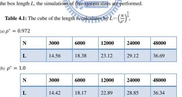
Using Monte-Carlo simulation for N particles in a cubic box of length L and with the periodic boundary conditions, we generate the configurations of the Lennard-Jones fluid with a linear term and with different cutoff distances [10]. Given in table 3.2 for different thermodynamic system we have done and in table 4.1 for the particle number N and the box length L, the simulations of five system sizes are performed.
Table 4.1: The cube of the length is calculates by L= ,
(a) N 3000 6000 12000 24000 48000 L 14.56 18.38 23.12 29.12 36.69 (b) N 3000 6000 12000 24000 48000 L 14.42 18.17 22.89 28.85 36.34
And we used the configurations to construct the 3N3N Hessian matrices. By using the JADAMILU package to solve the Hessian matrices, we achieve the eigenvectors and
the imaginary-frequency branch of INMs spectrum. At first, we roughly locate the ME by the property of and reveal the system-size invariance with the eigenvectors and eigenvalues receive from Hessina matrices. And, we are going on further analysis to check the universality of different thermodynamic states. Under the box-counting measuring, there are two different finite size scaling analysis methods: system-size scaling and box-size scaling. But the scaling behavior will breakdown for small box l near lattice constant a, the choice of small box size should be .
By average INMs of N=3000,6000,12000,24000 and 48000 at the ME in the imaginary-frequency branch and taking the ratio in the box-size scaling method as an integer varied from 2 to 8, we have calculated the and for q between -5 and 5. And in the system-size scaling, we defined l=2.427 in =0.972 and
l=2.403 in =1.0, it means in the simulated system of N=3000 was exactly partitioned into 216 boxes. For other larger simulated systems and with this l, L/l is not exactly an integer so that we partition each realization into small boxes of size l as many as possible, with some remains not enough to be a small box. Therefore, the five system sizes that we have simulated, the values of are 6,7,9,12 and 15. is maximum integer which is smaller than or equal to
L/ . And, we have calculated , the and for q between -6 and 5.9. Indicated our results, the maximum of occurred at on all the thermodynamic state have been showed in Table.(4.2).
With the data sets of and , the singularity spectrum at ME is shown in Fig.(4.1-4.5) Within numerical errors, the singularity spectrum at the ME is generally identical and agrees with the AM and the INMs at the ME of the short-range truncated Lennard-Jones fluid [37]. The results of SSP curve provide an evidence to confirm the location of the ME in the INMs spectrum. The reference figures all obtain from [40], the purpose is to compare with my data and confirm the mobility edges at different thermodynamics states still have the same properties. And, the ME at different
thermodynamic states are shown in Table.(4.3).
In conclusion, the system-size scaling is better than the box-size scaling in theory. Because the system-size scaling is exactly partitioned all the simulated system into equal size of small box. The box-size scaling is partitioned one simulated system into several unequal sizes of small boxes. Therefore, the fluctuation of the particle number between each small box for system-size scaling is much smaller than box-size scaling. From the view of our results, the system-size scaling is much sensitive to the precision of the ME frequency spectrum. Because it is hard to tell the different between the SSP curve at the frequency spectrum A and the frequency spectrum B. A and B frequency are all nearby the ME. Finally, we locate the exactly frequency of ME based on the system-size scaling result.
(All the reference data in Anderson model and INMs of TLJ fluid come from [38][39][40])
Table.(4.2) The ME at different thermodynamic states.
c ME( ) 2.5 0.972 0.836 -69.60.5 2.5 1.0 0.836 -70.40.5 2.5 1.0 0.7 -59.60.5 2.5 1.0 0.5 -43.30.5 3.5 0.972 0.836 -72.10.5
Table.(4.3) The position of the singularity strength (q=0) under box-size scaling and system-size scaling. (a) (b) Box-size System-size 3000 4.0940.0342 4.1770.0435 6000 4.0670.0306 12000 4.0520.0639 24000 4.0480.0262 48000 4.0830.0402 (c) (d) Box-size System-size 3000 4.0950.0557 4.0470.0224 6000 4.0850.0124 12000 4.0940.0178 24000 4.1140.0246 48000 4.1230.0406 (e) Box-size System-size 3000 4.0960.0138 4.1040.0346 6000 4.1060.0202 12000 4.1190.0375 24000 4.1270.0448 48000 4.1230.0101 Box-size System-size 3000 4.0390.0132 4.1090.0244 6000 4.0480.0312 12000 4.0750.0184 24000 4.0540.0252 48000 4.090.041 Box-size System-size 3000 4.1430.0378 4.0020.0491 6000 4.1780.0174 12000 4.1390.0274 24000 4.2170.0851 48000 4.2350.0435
Fig.(4.1-a) At thermodynamic state , the box-size scaling
of the singularity spectrum of the INMs LJ simple fluids at a ME. The INMs of
imaginary-frequency is calculated with (blue line with error bar). And, the circles, squares and red dashed line are all reference data come from [38][39][40].
Fig.(4.1-b) At thermodynamic state , the system-size
scaling of the singularity spectrum of the INMs LJ simple fluids at a ME. The INMs of imaginary-frequency is calculated with (green line with error bar) for five different system sizes from N=3000 to 48000. In each panel, is generated with the data of and with a step of .
Fig.(4.2-a) At thermodynamic state , the box-size scaling
of the singularity spectrum of the INMs LJ simple fluids at a ME. The INMs of
imaginary-frequency is calculated with (blue line with error bar). And, the circles, squares and red dashed line are all reference data come from [38][39][40].
Fig.(4.2-b) At thermodynamic state , the system-size scaling
of the singularity spectrum of the INMs LJ simple fluids at a ME. The INMs of imaginary-frequency is calculated with (green line with error bar) for five different system sizes from N=3000 to 48000. In each panel, is generated with the data of and with a step of .
Fig.(4.3-a) At thermodynamic state , the box-size scaling of
the singularity spectrum of the INMs LJ simple fluids at a ME. The INMs of imaginary-frequency is calculated with (blue line with error bar). And, the circles, squares and red dashed line are all reference data come from [38][39][40].
Fig.(4.3-b) At thermodynamic state , the system-size scaling of
the singularity spectrum of the INMs LJ simple fluids at a ME. The INMs of imaginary-frequency is calculated with (green line with error bar) for five different system sizes from N=3000 to 48000. In each panel, is generated with the data of and with a step of .
Fig.(4.4-a) At thermodynamic state , the box-size scaling of
the singularity spectrum of the INMs LJ simple fluids at a ME. The INMs of
imaginary-frequency is calculated with (blue line with error bar). And, the circles, squares and red dashed line are all reference data come from [38][39][40].
Fig.(4.4-b) At thermodynamic state , the system-size scaling of
the singularity spectrum of the INMs LJ simple fluids at a ME. The INMs of imaginary-frequency is calculated with (green line with error bar) for five different system sizes from N=3000 to 48000. In each panel, is generated with the data of and with a step of .
Fig.(4.5-a) At thermodynamic state , the box-size scaling
of the singularity spectrum of the INMs LJ simple fluids at a ME. The INMs of
imaginary-frequency is calculated with (blue line with error bar). And, the circles, squares and red dashed line are all reference data come from [38][39][40].
Fig.(4.5-b) At thermodynamic state , the system-size
scaling of the singularity spectrum of the INMs LJ simple fluids at a ME. The INMs of imaginary-frequency is calculated with (green line with error bar) for five different system sizes from N=3000 to 48000. In each panel, is generated with the data of and with a step of .
4.2 Singularity spectrum
In this section, we further compare the Singularity Spectrum curve at different thermodynamic states. Check to confirm if the SSP of INMs LJ fluids under different thermodynamic states still have invariance curve of . The results in Fig.(4.6) show that the SSP curve under different thermodynamic states almost consist with each other. But, the two edges of SSP curve (the spots at big |q| ) disperse to independent curve. We think that is
came from the gIPR to the power of big |q|. When the gIPR to the power of
|q| is big, it will amplify the numerical error in data base. If the average number of INMs can
be increased, the the numerical error in data base will be reduced. The SSP curve also will be able to perfectly consist with different thermodynamic states of INMs LJ fluid.
Fig(4.6-a) The system-size scaling of the singularity spectrum of the INMs LJ simple
fluids at a ME under different thermodynamic states. These thermodynamic states already have showed in Table.4.3.
Fig(4.6-b) The box-size scaling of the singularity spectrum of the INMs LJ simple
fluids at a ME under different thermodynamic states. The results of five different simulated system sizes from N=3000 to 48000 show in order. These thermodynamic states already have showed in Table.4.3.
4.3Probabilty density function of vibrational amplitudes
The probability density function of vibrational amplitudes is calculated with 7000-9000 INM eigenvectors for each N from 3000 to 48000. The variation of with each system size is shown in Fig(4.6-4.10). The position of the maximum is almost invariant with system size. Within numerical resolution, this maximum position almost located at , it is very close to the value of obtained from the box-size scaling and system size scaling. Moreover, we used the Eq.(2.3.14) to calculate the singularity spectrum , and all the results showed in Fig(4.6(b)-4.10(b)).
The reason why we let the probability density function of vibrational amplitudes become a method to locate the position of ME is the maximum point of must be locate at . Because the SSP curve at , . When this situation occurred, it means that it is the spot closest the extended mode and the number of particle are the most. The meanings are the same. But this method still has a disadvantage. The discrete numerical point of will induce numerical error for PDF. So, the precision of must been influenced by the average number of INMs and the numerical resolution ( ). If the average number of INMs can increase, the numerical resolution can be smaller and the curve of PDF does not become rough. Our results have showed this situation at some thermodynamic states. It means that the position of do not consist with different simulated system and the relation between the maximum value of ) and is not linear.
Fig.(4.7-a) At thermodynamic state , the probability
density function of vibrational amplitudes change with different simulated system size for INMs LJ fluids at . . The numerical results with the resolution equal to 0.05. And, the inset shows versus and fit of (red solid line), with A= 0.026988 and B=0.27511.
Fig.(4.7-b) At thermodynamic state , the singularity
spectrum of the INMs LJ simple fluids at a ME obtained by
(Eq.(2.3.14)) with five different simulated system sizes from 3000 to 48000. And, the circles, squares and red dashed line are all reference data come from [38][39][40].
Fig.(4.8-a) At thermodynamic state ,the probability density
function of vibrational amplitudes change with different simulated system size for INMs LJ simple fluids at . . The numerical results with the resolution equal to 0.05. And, the inset shows versus and fit of (red solid line), with A= 0.0833 and B=0.2462.
Fig.(4.8-b) At thermodynamic state , the singularity
spectrum of the INMs LJ fluids at a ME obtained by
(Eq.(2.3.14)) with five different simulated system sizes from 3000 to 48000. And, the circles, squares and red dashed line are all reference data come from [38][39][40].
Fig.(4.9-a) At thermodynamic state , the probability density
function of vibrational amplitudes change with different simulated system size for INMs LJ fluids at . . The numerical results with a resolution equal to 0.05. And, the inset shows versus and fit of (red solid line), with A= 0.082 and B=0.2455.
Fig.(4.9-b) At thermodynamic state , the singularity spectrum
of the INMs LJ fluids at a ME obtained by
(Eq.(2.3.14)) with
five different simulated system sizes from 3000 to 48000. And, the circles, squares and red dashed line are all reference data come from [38][39][40]..
Fig.(4.10-a) At thermodynamic state , the probability density
function of vibrational amplitudes change with different simulated system size for INMs LJ fluids at . . The numerical results with the resolution equal to 0.05. And, the inset shows versus and fit of (red solid line), with A= 0.1028 and B=0.228.
Fig.(4.10-b) At thermodynamic state , the singularity spectrum
of the INMs LJ fluids at a ME obtained by
(Eq.(2.3.14)) with
five different simulated system sizes from 3000 to 48000. And, the circles, squares and red dashed line are all reference data come from [38][39][40].
Fig.(4.11-a) At thermodynamic state , the probability
density function of vibrational amplitudes change with different simulated system size for LJ fluids INMs at . . The numerical results with the resolution equal to 0.05. And, the inset shows versus and fit of (red solid line), with A= 0.0686 and B=0.246.
Fig.(4.11-b) At thermodynamic state , the singularity
spectrum of the INMs LJ fluids at a ME obtained by
(Eq.(2.3.14)) with five different simulated system sizes from 3000 to 48000. And, the circles, squares and red dashed line are all reference data come from [38][39][40].
Chapter5
5.Conclusions
In this paper, we have investigated the multifractality of the INMs at the imaginary-frequency branch ME of simple fluids. The locations of the MEs are determined by the invariance of the singularity spectrum (SSP) and the maximum position in the probability density function of vibrational amplitudes with the system size. We generalize the multifractal analysis for the INMs at a ME with the box-counting method for the LJ fluids at different thermodynamic states. In the box-counting method, the simulated system is partitioned into equal-volume small boxes. The multifractal analysis under typical ensemble is performed for both the box-size scaling and the system-size scaling. By the box-size scaling and the system-size scaling, the singularity spectrum of the multifractal INMs agree with the results calculated for the AM and the short-range interaction fluid. Moreover, the SSP curve consist with different thermodynamic states in INMs LJ simple fluids. Therefore, we can confirm that the SSP is a universal quantity. But, the SSP under the system-size scaling is more sensitive for predicting the precise location of the ME. So, we suggest the system-size scaling for determining the imaginary-frequency branch ME.
The probability density function of vibrational amplitudes provides another method to determine the location of ME. But, this method is influenced in numerical resolution by the average number of the INMs, which means that the average total number of INMs that we have calculated for each system size in our researches are not enough to reduce the fluctuation in the values of and . Also, the precision of and the SSP curve calculated by PDF of vibrational amplitudes can not compare with the MFA. Especially, the SSP curve
calculated by PDF of vibrational amplitude on two edges of curve (big ) do not consist with the AM and short-range interaction fluid.
In conclusions, these two methods perform well in the researches on this subject. The precision of the SSP curve and probability density function of amplitudes would be better as long as the average number of INMs is enhanced in 2 or 3 orders. The other direction is to increase the simulated system size to check whether the universality still exists. In principle, these improvements will produce higher precisions in numerical data by reducing error bars. We still need to overcome the formidable system size effect on the real-frequency ME and solve the crystallization problem of a simple fluid at high densities or low temperatures. These problems are still considerable issues. Moreover, let the multifractal analysis apply to the other physic system, because the multifractal analysis has the advantage in theory to be easy and understandable. The most importance is that the multifractal theory is easier to be realized than the complicated many-body theories for realistic physical systems.
Appendix A
A.1 Derivation for Legendre Transform of SSP from the
Mass Exponents
Generally, the general inverse participation ratio scales with system size as
(A.1) where is the mass exponent. Here, we derive the Legendre transform . Consider the LPD defined in Eq.(2.3.5), in the discrete system satisfies the normalized condition , where . The probability density function of the LPD is defined as
,
where is the number of boxes with within [ ]. The is normalized as,
By changing variable to the singularity strength
,
the corresponding PDF . The PDF of should also satisfy the normalization condition
After changing variable to the singularity strength, the definition of the gIPR become
Based on the definition of fractal dimension N~L f(), where N is the numberof boxes belong to [ ], and the probability of within [ ] is . Therefore, we have
. Consequently,
(A.2) Evaluation of the integral by the saddle-point method gives
(A.3) which reproduce Eq.(A.1), with the mass exponent related to the singularity spectrum via the Legendre transform
Bibliography
[1] F. Evers and A. D. Mirlin, Rev. Mod. Phys. 80, 1355 (2008).
[2] J. Billy, V. Josse, Z. Zuo, A. Bernard, B. Hambrecht, P. Lugan, D. Clement, L. Sanchez –Palencia, P. Bouyer, and A. Aspect, Nature (London) 453, 891 (2008).
[3] G. Roati, C. D’Errico, L. Fallani, M. Fattori, C. Fort, M.Zaccanti, G. Modugno, M. Modugno, Nature 453, 895 (2008).
[4] H. Hu, A. Strybulevych , J. H. Page, S. E. Skipetrov, and B. van Tiggelen, Nat. Phys. 4, 945 (2008)
[5] A. Lagendijk, B. van Tiggelen, and D.S. Wiersma, Phys. Today 62(8), 24(2009) [6] A. Aspect and M. Inguscio, Phys. Today 62(8), 30 (2009)
[7] A. Richardella, P. Roushan, S. Mack, B. Zhou, D. A. Huse, D. D. Awschalom, and Yazdani, Science 327, 665 (2010)
[8] W. Garber, F. M. Tangerman, P. B. Allen, and J. L. Feldman, Philos. Mag. Lett. 81, 433(2001)
[9] J. J. Ludlam, S. N. Taraskin , and S. R. Elliott, Phys. Rev. B 67, 132203 (2003) [10] J. L. Feldman and N. Bernstein, Phys. Rev. B 70, 235214
[11] J. J. Ludlam, S. N. Taraskin , and S. R. Elliott, J. Phys.: Condens. Matter 17, L321 (2005) [12] S. Faez, A. Strybulevych, J. H. Page, A. Lagendijk, and B. A.van Tiggelen , Phys. Rev.
Lett. 103,155703 (2009)
[13]B. J. Huang and T. M. Wu, “Localization-Delocalization Transition in Hessian Matrices of Topologically Disordered Systems”, Phys. Rev. E 79, 041105 (2009)
[14] T. M. Wu and R. F. Loring, “Phonons in liquids: A random walk approach”, J. Chem. Phys. 97, 8568(1992).
[15] E. La Nave, A. Scala, F. W. Starr, G. E. Stanley, and F. Sciortino, “Dynam- ics of Supercooled Water in Configuration Space”, Phys.Rev. E 64, 036402 (2001).
[16] T. M. Wu, S. L. Chang, and K. H. Tsai, “Mechanism” for singular Behavior in Vibrational Spectra of Topologically Disoedered Systems: Short-Range Attractions”, J. Chem. Phys. 122, 204501(2005).
[17] W. J. Ma, T. M. Wu, and J. Hsieh, “Conservation Constraints on Random Matrices”, J. Phys. A 36, 1451(2003).
[18] D. A. Parshin and H. R. Schober, “Multifractal Structure of Eigenstates in the Anderson Model with Long-Range Off-Diagonal Disorder”, Phys. Rev. B 57, 10232(1998).
[19] S. N. Taraskin, Y. L. Loh, G. Natarajan, and S. R. Elliot, “Origin of the Boson Peak in Systems with Lattice Disorder”, Phys. Rev. Lett. 86, 1255 (2001).
[20] J. J. Ludlam, S. N. Taraskin, and S. R. Elliot, “Disorder-InducedVibrational Localization”, Phys. Rev. B 67, 132203(2003).
[21] W. Schirmacher, G. Diezemann and C. Ganter, “Harmonic Vibrational Exc- itations in Disordered Solids and the Boson Peak”, Phys. Rev. Lett. 81, 136 (1998).
[22] M. Mezard, G. Parisi, and A. Zee, “Spectra of Euclidean Random Matrices” ,Nucl. Phys. B 559, 689(1999).
[23] T.M. Wu and R.F. Loring, J.Chem. Phys. 97,8568
[24]M. Bollhöfer and Y. Notay, Computer. Phys. Commun.177,951(2007)
[25]O. Schenk,M. Bollhöfer, and R. A. Römer, SIAM J. Sci. Comput. (USA) 28, 963 (2006) [26]B. J. Huang and T. M. Wu, “Localization-Delocalization Transition in Hessian Matrices
[27]T. M. Wu, W. J. Ma, “Evidence for instantaneous resonant modes in dense fluids with repulsive Lennard-Jones force“, J. Chem. Phys. 110, 447(1999) [28] X. Jia, A. R. Subramaniam, I. A. Gruzberg, and S. Chakravarty, “Entang-
lement Entropy and Multifractality at Localization Transitions”, Phys. Rev. B 77, 014208(2008).
[29] L. Gong and P. Tong, “Localization-Delocalization Transitions in a Two- Dimensional Quantum Percolation Model: Von Neumann Entropy Studies”, Phys. Rev. B 80, 174205(2009).
[30] B. J. Huang and T. M. Wu,“Numerical studies for localization-delocalization transition in vibrational spectra”, Comput. Phys. Commum. 182, 213 (2011).
[31] T. C. Halsey, P. Meakin and I. Procaccia, “Scaling Structure of the Surface Layer of Diffusion-Limited Aggregates”, Phys. Revv. Lett. 56, 854(1986). [32] C. Amitrano, A. Coniglio and F. di Liberto, “Growth Probability Distribu-
tion in Kinetic Aggregation Processes”, Phys. Rev. Lett. 57, 1016(1986). [33] T. C. Halsey, M. H. Jensen, L. P. Kadanoff, I. Procaccoa, and B. I. Shraiman
, “Fractal Measures and Their Singularities: The Characterization of Stran- ge Sets”, Phys. Rev. A 33, 1141(1986).
[34] F. Milde, R. A. R mer, and M. Schreiber, “Multifractal Analysis of the Met- al Insulator Transition in Anisotropic Systems”, Phys. Rev. B 55,9463 (1997).
[35] H. Grussbach and M. Schreiber, “Determination of the Mobility Edge in the Anderson Model of Localization in Three Dimensions by Multifractal Ana-
lysis”, Phys. Rev. B 51, 663(1995).
[36] M. Schreiber and H. Grussbach, “Multifractal Wave Functions at the Ander- son Transition”, Phys. Rev. Lett. 67,607(1991).