M-estimator based Robust Radial Basis Function Neural Networks with Growing and Pruning Techniques

全文

(1)M-estimator based Robust Radial Basis Function Neural Networks with Growing and Pruning Techniques Chien-Cheng Lee*, Chun-Li Tsai**, Yu-Chun Chiang***, and Cheng-Yuan Shih * * Department of Communications Engineering, Yuan Ze University, Chungli, Taoyuan 320, Taiwan cclee@saturn.yzu.edu.tw ** Department of Economics, National Cheng Kung University, #1 University Road, Tainan, 701, Taiwan *** Department of Mechanical Engineering, Yuan Ze University, Chungli, Taoyuan 320, Taiwan. ABSTRACT In this paper, we present an M-estimator based robust radial basis function (RBF) learning algorithm with growing and pruning techniques. The Welsch M-estimator and median scale estimator are employed to avoid the influence from outliers. The concept of neuron significance is adopted to implement the growing and pruning techniques of network nodes. The proposed method not only eliminates the influence of the outliers, but also dynamically adjusts the number of neurons to approach an appropriate size of the network. The results from experiments show that the proposed method can give a minimum prediction error compared with other methods. Furthermore, even 30% of all observations are the outliers this method still has a good performance.. 1: INTRODUCTION The radial basis function (RBF) neural network is considered as a good candidate for approximation and prediction problems due to its rapid learning capacity. In typical RBF networks, the Gaussian function is selected as the activation function of network. A network iteratively adjusts parameters of each node by minimizing the LMS (least-mean-square) criterion according to gradient descent algorithm. Nevertheless, there still exist some problems in this approach. When some of the training patterns contain large errors resulting from the presence of outliers, the network will yield inadequate responses in the neighborhood of the outliers due to the MSE criterion. Another frequently encountered problem for neural networks is that it is difficult to determine the number of neurons of the network. If the number of centers is underestimated, the capability of the network is limited and the performance therefore might be degraded. On the other hand, if the number of centers is over-determined, a large network is generated and an increase in time is required for the network process. In order to take care of these two. problems, an M-estimator based robust RBF learning algorithm with growing and pruning techniques is introduced in this paper. M-estimator statistics is a widely used robust statistics [1]-[7]. It uses some cost functions which increase less than that of least square estimators as the residual departs from zero. When the residual error goes beyond a threshold, the M-estimator suppresses the response instead. Therefore, the M-estimator based error function is more robust for the presence of the outliers than LMS based error function. M-estimator replaces the MSE criterion and then provides the robustness for the traditional neural networks. The simulation results show that the proposed method can produce the minimum prediction error than other methods, even outliers are included. The optimal size of network for a given problem is usually unknown. If the number of neurons is underestimated, the network may not approximate or predict the problem accurately. On the other hand, if too many neurons are used, the network will overfit the training pattern, result in inferior outcome, and also increase the computation time. In the past, several methods for growing and pruning in RBF networks have been proposed [8]-[11]. Huang et al. [11] proposed a concept of significance of a neuron, which is wholly different from and much simpler than other methods. The significance is defined as a neuron’s statistical contribution to the overall performance of the network, and it is used in growing and pruning strategies. A new neuron will be added only if its significance is larger than the chosen threshold. Conversely, if the significance for a neuron is less than the threshold, the neuron will be pruned. In this paper, we adopt this concept of the significance of a neuron to define the network growing and pruning algorithm. According to the approach, the network can produce a proper size for a given problem. The paper is organized as follow. The M-estimator based radial basis function neural network and the growing and pruning techniques are given in Section 2.. - 1065 -.

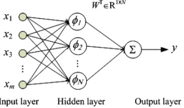
(2) The simulation results are conducted in Section 3. Finally, conclusions are included in Section 4.. 2: M-ESTIMATOR BASED RADIAL BASIS FUNCTION NEURAL NETWORKS 2.1: BASIC ARCHITECTURE OF RADIAL BASIS FUNCTION NETWORKS The basic architecture of an RBF network is a single hidden layer feed forward neural network, as shown in Fig.1.. where rn= d(n)- y(n) represents the residual error between the desired, d(n), and the actual network outputs, y(n). n indicates the index of the series. The cost function can be defined as an ensemble average errors, J (θ ) = E [ρ ( rn )] (3) where θ is one of the parameter sets of the network. According to the gradient descent method, the gradient of the cost function J(θ) needs to be computed. The gradient surface can be estimated by taking the gradient of the instantaneous cost surface. That is, the gradient of J(θ) is approximated by Eq (4) ∂J (θ ) ∂ρ (rn ) ∂rn ≈ ∇θ J (θ ) = (4) ∂θ ∂rn ∂θ where. ∂ρ (rn ) = rn ∂rn. (5). and. Fig. 1. Basic architecture of RBF neural network The output of the RBF network is described by. y = f ( x ) = ∑ wkφk ( x − c k ,σ k ). ∂y ∂rn =− . (6) ∂θ ∂θ The update equation for the network parameters is given by ∂ ∂y J (θ ) ≈ θ (n) + μθ rn θ (n + 1) = θ (n) − μθ . (7) ∂θ ∂θ The cost function is not necessary defined as LMS criterion; that is, we can define the influence function as. ψ (rn ) =. N. (1). k =1. where y is the actual network output, x∈R is an input vector signal, with individual vector components given as xj, for j=1, 2, …,m, that is, x=[x1, x2, …, xm]T ∈Rm×1. w=[ w1, w2, …, wN]T ∈RN×1 is the vector of the weights in the output layer, N is the number of neurons in the hidden layer, and φk(⋅) is the basis function of the network from Rm×1 to R. ck=[ ck1, ck2, …, ckm]T ∈Rm×1 is called the center vector of the kth node, k is the bandwidth of the basis function φk(⋅), and ||⋅|| denotes the Euclidean distance. For each neuron in the hidden layer, the Euclidean distance between its associated center and the input to the network is computed. The output of the neuron in a hidden layer is a nonlinear function of the distance, and the Gaussian function is most widely selected as the nonlinear basis function. After the computation of the output for each neuron, the output of the network is computed as a weighted sum of the hidden layer outputs. In the training procedure, the steepest gradient of descent learning process is to adjust the appropriate settings of the parameters (e.g. weights, centers, and bandwidths), which make the performance of the network mapping optimized. A common optimization criterion is to minimize the LMS between the actual and desired network outputs. LMS error function is as Eq (2), 1 ρ (rn ) = rn2 (2) 2 m×1. ∂ρ (rn ) . ∂rn. (8). We rewrite Eq (7), the generalized update equation is the following ∂y θ (n + 1) = θ (n) + μθψ (rn ) . (9) ∂θ. 2.2: M-ESTIMATOR LEARNING RULE. BASED. RBF. Most of the learning rules of neural networks are based on the LMS criterion, which minimize the quadratic function of the residual errors. However, LMS is not a good criterion for some training patterns in which there exist huge errors by the presence of outliers. Those errors cause the training patterns move far away from the underlying position. Consequently, approximations can’t be precise. To illustrate this problem, we give an example to show the weakness of LMS criterion in the case of outliers. We generate the sine function, which includes 200 training data. 18 outliers are randomly selected and 12 neurons are used in the network training. After 400 training iterations by traditional RBF network, the RMSE is 0.1413 and the approximation result is shown in Fig. 2. The influence function in LMS criterion (ψ(rn)= rn) is linearly with the size of its error. Seeing Fig. 2, we can find the outliers magnify the influence values. Thus, it is not a good approximation by using LMS criterion in this case of outliers. Recalling Eq (7), the network updates are proportional to the linear influence function ψ(rn). It. - 1066 -.

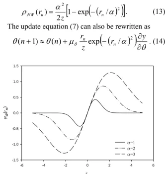
(3) ρ NW ( rn ) =. [1 − exp(− (r / α ) )]. 2z. α2. 2. (13). n. The update equation (7) can also be rewritten as. θ ( n + 1) ≈ θ ( n ) + μ θ. (. ). rn 2 ∂y . (14) exp − (rn / α ) z ∂θ. 1.5. 1.0. 0.5. ψw(rn). would offer the key to an understanding of overcoming the outlier problem. One possible solution for improving this problem is to employ a robust criterion instead of LMS. Among several methods, which deal with the outlier problem, M-estimator technique [1], [2] is the most robust and has been applied in many applications [3]-[6]. The M-estimator uses some cost functions which increase less rapidly than that of least square estimators as the residual departs from zero. When the residual error increases over a threshold, the M-estimator suppresses the response instead. Therefore, the M-estimator based error function is more robust to outliers than LMS based error function.. 0.0. -0.5. Desired output Outlier Network output. 1.5. α=1 α=2 α=3. -1.0. 1.0. -1.5 -6. -4. -2. 0. 2. 4. 6. rn. 0.5 Y. Fig. 3. Influence function ψw(⋅) with different spread parameters. 0.0. -0.5. -1.0 0. 2. 4. 6. 8. 10. 12. 14. 16. 18. X. Fig. 2. The approximation result when training patterns contain outliers. The learning rules of neural networks were based on the LMS criterion Several M-estimators have been studied [1]-[7] including Huber, Cauchy, Geman-McClure, Welsch, and Tukey. In our paper, we employ the Welsch function as the error function, given by. α2. [. (. )]. (10) 1 − exp − (rn / α ) 2 where α is a scale parameter. The corresponding influence function can be given by dρ ( r ) ψ W (rn ) = W n = rn exp − (rn / α )2 . (11) drn The Influence function ψw(⋅) with different scale parameter α is plotted in Fig. 3. From Fig. 3, the output of influence functions varies with respect to scale parameter. For example, the maximum values of ψw(⋅) are 1.287, 0.858, and 0.429 for α=3, 2, and 1, respectively. This experiment causes the fraction of network parameter update is difficult to control. To solve this problem, a normalization factor z is employed to normalize the function output to [-1, 1]. We rewrite Eq (11) as. ρW (rn ) =. 2. (. ψ NW (rn ) =. (. (. rn exp − (rn / α ) z. ). ). 2. ). (12). where z = exp − (1 / α )2 , and Eq (10) can be also rewritten as. Furthermore, Fig. 3 also indicates the interval among the extreme points of ψw(⋅). The interval can be regarded as the confidence interval of the residuals. In other words, if the residual error falls into this interval, the estimate is proportional to the size of the error; otherwise, the data is treated as an outlier and the update is suppressed. The extreme points can be detected by letting dψw (rn)/drn =0, that is, ∂ψ NW ( rn ) 1 2 2 = 1 − 2(rn / α ) exp − (rn / α ) = 0 .(15) ∂rn z −0.5 Obviously, the extreme points are ± 2 α , and the −0.5 −0.5 confidence interval is the range [ − 2 α , 2 α ]. The. (. ) (. ). interval depends on the scale α. When α is large, outliers may not be discriminated from the majority. Conversely, if α is small, some of desired data will be treated as outliers. We use a median operator to estimate the scale, since it is simple to understand and easy to calculate. Furthermore, it also gives a more robust measure in the presence of outlier values than the mean value [7].. 2.3: GROWING TECHNIQUES. AND. PRUNING. Another major challenge in this design of the robust RBF neural network is to determine the number of the centers. Huang et al. [11] have proposed the concept of significance of a neuron, which is wholly different from and much simpler than other methods. The significance is defined as a neuron’s statistical contribution to the overall performance of the network, and it is used in growing and pruning strategies. A new neuron will be added only if its significance is larger than the chosen threshold. Conversely, if the significance for a neuron becomes less than the threshold, then that neuron will be pruned. In this paper, we adopt the concept of the. - 1067 -.

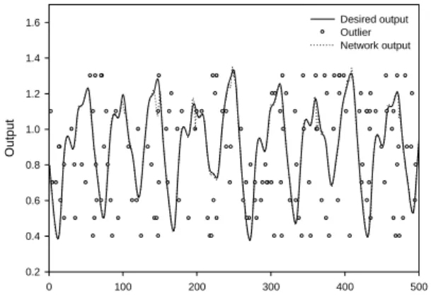
(4) significance of a neuron to define the network growing and pruning algorithm. To define the significance of a neuron for pruning (SNP), we assume the output of a RBF network with N neurons for an input x is given by (1). If the neuron q is removed, the output of the RBF network with the remaining N-1 neurons is k =1. ∑w φ ( x − c N. k = q +1. k k. k. ,σ k ) (16). Therefore, for an input xi the error resulting from removing neuron q is the absolute difference between y and yq, that is PErr (i, q ) = y − y q = wq φ q x i − c q , σ q (17). (. ). The significance of a neuron for pruning is defined as the average error for all M sequentially learned inputs due to removing neuron q, given by. 1.6 Desired Output Network Output 1.4. 1.2. 1.0. Output. q −1. yq = ∑ wkφk ( x − ck ,σ k ) +. To further examine the advantage of the robustness of our proposed RBF neural network, 30% of training data are replaced by random outliers to test the capability of the anti-outlier. Fig. 5 shows the results of the training phase, and the corresponding RMSE is 0.027035. The results show that it is nearly equal to the result of Kim and Kim’s method even there is no outlier included.. 0.8. 0.6. M. SNP(q) =. ∑ PErr(i, q) i =1. M. 0.4. =. wq M. ∑φ ( x M. i =1. q. i. − cq ,σ q. ). (18). 0. If SNP(q) < TPErr (TPErr is a predefined threshold value), it means the neuron q does not make significant contribution to the overall performance of the network; hence, this neuron should be removed. Similarly, the rule of growing node can be defined by this way.. 3: SIMULATION RESULTS PERFORMANCE EVALUATION. 0.2 100. 150. 200. 250. 300. 350. 400. 450. 500. Time. Fig. 4. Mackey-Glass Chaotic Time Series Prediction. AND. We examine the performance of the proposed M-estimator on the prediction of one time series data. The data is generated by the chaotic Mackey-Glass differential delay function as dx(t ) 0.2 x(t − τ ) = − 0.1x(t ) dt 1 + x10 (t − τ ) (19). Method. Prediction Error (RMSE). Iterations. Our Method Traditional RBF (with 19 neurons) ANFIS Backpropagation NN Auto Regressive Model Kim and Kim (Ensemble). 0.006807 0.011526. 500 500. 0.007 0.02 0.19. 500 500 500. 0.0262431. 500. Table 1. Comparison results of the prediction error of different methods. Desired output Outlier Network output. 1.6 1.4 1.2. Output. where >17. In this experiment, 1500 points are generated with an initial condition x(0)=1.2 and =17. 500 points of the series data are generated from x(100)-x(599) and used as training data, and the other 500 points are generated from x(600)-x(1099) and used to validate the prediction performance. The networks are employed to predict the values of the time series at point x(t) from the four past samples [x(t-6), x(t-12), x(t-18), x(t-24)]. Two neurons are given in the beginning of the training, and the corresponding centers are uniformly assigned from data range. The initial weights are randomly selected from [-0.3, 0.3], and the total number of training iterations is set to 500. Fig. 4 shows the test result of noise-free time series using the proposed method, and the RMSE is 0.006807. The number of neurons dynamically increases from 2 to 19. Table 1 shows the comparison results of the prediction performance among different methods including our proposed method. The data of last four rows in Table 1 are taken from [12]. From the comparison results, we can see that our proposed algorithm results in the smallest prediction error than other methods.. 50. 1.0 0.8 0.6 0.4 0.2 0. 100. 200. 300. 400. 500. Time. Fig. 5. Training results of 30% of training data are replaced by random outliers. - 1068 -.

(5) 4: CONCLUSIONS In this paper, we have successfully proposed an M-estimator based robust RBF neural network with growing and pruning techniques to predict the noisy time series. The Welsch M-estimator and median scale estimator are employed to avoid the influence from the outliers. The concept of significance of a neuron is adopted to implement the growing and pruning techniques of network nodes. The results show that the proposed method not only eliminates the influence of the outliers but also dynamically adjusts the number of neurons to approach an appropriate size of the network. In the experiment of time series prediction, the proposed method results in the minimum prediction error than other methods. The experiment also shows that even the observations contain the outliers of 30 % this method still has a good performance.. IEEE Trans. Syst., Man, Cybern. B, vol. 34, no. 6, pp. 2284-2292, 2004. [12] D. Kim, and C. Kim, “Forecasting time series with genetic fuzzy predictor ensemble,” IEEE Trans. Fuzzy Syst., vol. 5, no. 4, pp.523-535, 1997.. Acknowledgments. The authors would like to thank the National Science Council for supporting this work under the Grant number NSC 94-2213-E-155 -049.. REFERENCES [1] P. J. Huber, Robust Statistics, John Wiley and Sons, New York, 1984. [2] T. Barnett and Lewis, Outliers in Statistical Data, John Wiley and Sons, New York, 1994. [3] J. H. Chen, C. S. Chen, and Y. S. Chen, “Fast algorithm for robust template matching with m-estimators,” IEEE Transactions on Signal Processing, vol. 51, no. 1, pp.230–243, 2003. [4] L. Mangasarian and D. R. Musicant, “Robust linear and support vector regression,” IEEE Transactions on Pattern Analysis and Machine Intelligence, vol. 22, pp. 950–955, 2000. [5] C. C. Lee, P. C. Chung, J. R. Tsai, and C. I. Chang, “Robust Radial Basis Function Neural Networks,” IEEE Trans. Syst., Man, Cybern. B, vol. 29, no. 6, pp. 674-684, 1999. [6] X. Hong and S. Chen, “M-Estimator and D-Optimality Model Construction Using Orthogonal Forward Regression,” IEEE Trans. Syst., Man, Cybern. B, vol. 35, no. 1, pp. 155–162, 2005. [7] P. J. Rousseeuw and S. Verboven, “Robust estimation in very small samples,” Computational Statistics & Data Analysis, vol. 40, pp. 741-758, 2002. [8] S. Chen, C. F. N. Cowan, and P. M. Grant, “Orthogonal least squares learning algorithm for radial basis function networks,” IEEE Trans. Neural Netw., vol. 2, no. 2, pp. 302-309, 1991. [9] S. Chen, E. S. Chng, K. Alkadhimi, “Regularized orthogonal least squares algorithm for constructing radial basis function networks,” Int. J. Control, vol. 64, no. 5, pp. 829-837, 1996. [10] M. J. L. Orr, “Regularization on the selection of radial basis function centers,” Neural Computat., vol. 7, pp. 606-623, 1995. [11] G. B. Huang, P. Saratchandran, and N. Sundararajan, “An Efficient Sequential Learning Algorithm for Growing and Pruning RBF (GAP-RBF) Networks,”. - 1069 -.

(6)