Analyzing accelerated degradation data by nonparametric regression

IEEE TRANSACTIONS ON RELIABILITY, VOL. 48, NO. 2, 1999 JUNE 149

Analyzing Accelerated Degradation Data

By

Nonparametric Regression

Jyh-Jen Horng Shiau

National Chiao Tung University, Hsinchu

Hsin-Hua Lin

National Chiao Tung University, Hsinchu

Key Words

-

Accelerated degradation test, Acceleration factor, Accelerated life-stress degradation model, Local lin-

ear regression smoother, Nonparametric regression, Stochastic process.

Summary & Conclusions - This paper presents a non- parametric regression accelerated life-stress (NPRALS) model for accelerated degradation data wherein the data consist of

groups of degrading curve data. In contrast to the usual para- metric modeling, a nonparametric regression model relaxes as-

sumptions on the form of the regression functions and lets data speak for themselves in searching for a suitable model for

data. NPRALS assumes that various stress levels affect only the degradation rate, but not the shape of the degradation

curve. An algorithm is presented for estimating the compo- nents of NPRALS. By investigating the relationship between the acceleration factors and the stress levels, the mean time to failure estimate of the product under the usual use condition is obtained. The procedure is applied to a set of data obtained from an accelerated degradation test for a light emitting diode product. The results look very promising. The performance of NPRALS is further checked by a simulated example and found satisfactory. We anticipate that NPRALS can be applied to other applications as well.

1.

INTRODUCTION

Acronyms' LED ' ADT LLR PC PCA PCBF MTTF SAFT

SL

SLI NPRALS

light emitting diode accelerated degradation test local linear regression principal component ' P C analysis

P C basis function mean time to failure scale accelerated failure time stress level

standardized light intensity the model in this paper

In many experiments in life sciences and engineering, the collected data are samples of response curves. Growth data of children is an example, and degradation data of

'The singular & plural of an acronym are always spelled the same.

a product-performance measure is another. How to ana- lyze such data has become important in recent statistical research.

Due to rapid advances of technology and to quality im- provement efforts, many products are so reliable that tra- ditional life tests are not feasible in estimating the lifetimes

of these products. In such circumstances, accelerated tests are widely used to shorten the life of products or hasten the degradation of their performance. The aim of such tests is to collect data quickly so that desirable informa- tion on product life or on performance under usual use can be obtained in a reasonable time by appropriate modeling and analysis.

This study focuses on accelerated degradation tests (ADT) data analysis. Most of the ADT analyses use para- metric regression models to estimate the lifetime of the product under usual use. To relax the assumptions on the form of regression functions and let data speak for them- selves in searching for a suitable model for data,,we pro- pose a nonparametric regression model to analyze ADT data in this paper.

Nonparametric regression techniques are useful in ob- taining a smooth fit to noisy data, to describe the re- lationship between response variables and s-independent variables. These smoothing techniques are powerful tools in statistical data-analysis because of the,

model flexibility,

-

appealing look of the fitted curves (or surfaces). Several books were published in recent years on smoothing techniques, eg, [2 - 6, 131.

1.1 Relevant Works

Recently, many researchers have paid much attention to modeling & analyzing degradation data. Nelson [ll] pro- vided a fairly thorough survey on ADT, which included ar- eas of applications, statistical models, and data analyses. Meeker & Escobar [8] reviewed recent research in acceler- ated testing. Lu & Meeker [7] used a non-linear mixed- effects model with degradation data to estimate the life distribution. Meeker, Escobar, Lu

[lo]

presented meth- ods for analysis of accelerated degradation data. They used approximate maximum likelihood estimation to es- timate model parameters from the assumed mixed-effects 0018-9529/991$10.00 01999 IEEE

150 IEEE TRANSACTIONS ON RELIABILITY, VOL. 48, NO. 2, 1999 JUNE

nonlinear regression model; and they suggested methods for estimating lifetime distributions for various situations. Meeker & Escobar (91 presented many up-to-date statisti- cal methods for analyzing reliability data.

In life sciences, Capra & Muller [l] proposed an acceler- ated time model for cohorts of female Mediterranean fruit flies that may age faster or slower, depending on inher- ent genetic dispositions or external factors like varying temperature and humidity.

A

nonparametric regression method was used to estimate the mean mortality function under usual conditions.

For more research on this topic, see [l, 7 - 111. 1.2 The Motivated Application

Our research was motivated by a set of ADT data on LED. LED have been widely used in many fields, rang- ing from consumer electronics to optical fiber transmis- sion systems. LED has many nice features, such as less power consumption, small volume, good visual effect, and long lifetime. Applications include electronic boards on highways and on streets, smoke sensors on ceilings, night lights, and traffic lights. LED products are gradually re- placing traditional light bulbs in many places. Because of the very-high-reliability of LED products, it is difficult to obtain information on product life under usual use in a short time.

Yu & Tseng [14] proposed an on-line procedure for ter- minating an ADT experiment. They applied the procedure on a set of ADT data of an LED product with electric current as the accelerating variable. This study analyzes another set of ADT data of the same LED product with temperature as the accelerating variable. Our goal is to es- timate the MTTF of the product under usual use. Section

4 describes this LED data set in more detail. 1.3 Overview

Section 2 introduces the NPRALS model. Section 3 pro- poses an algorithm for estimating the components of this model. Section 4 performs a data analysis on a set of ADT data of an LED product based on NPRALS. Section 5 has a simulation study to explore the effectiveness of NPRALS and reports the results. Section 6 discusses the resulting situation.

Notatzon

m number ofSL

i

n, j p k

tk

& , j , k

tz,j,k

T

index for SL,

i

= 1,.

. .

,

m

number of test items for SL

i

index for test items, j = 1 , .

.

.

,

n,

number of measurements for each test item index for the measurements, k = 1 , .

.

.

, p

measurement time for measurement k of

measurement for item j under SL

i

at

tk

measurement time for

Xz,3,k;

tz,j,k

=

tk

for a closed interval of time

each test item

each i , j

A implies an estimate

acceleration factor (or relative acceleration rescaled time for

ti,j,k

according to

&

measurement corresponding to

t : , j , k ;

stochastic process of quality characteristic,

factor after scaling) for SL i

x,!,j,k =

Xi,j,k

mean function of

X

(.)

stochastic process with mean zero, and T ( . ,

.)

covariance of W (

.)

measurement/experimental error index for PCBF; q = 1,.

. .

,

L

number of PCBF PCBF q of

X ( . )

for SL

i

random coefficient of

sample covariance matrix for SL i

MTTF under SL

i

absolute temperature for SL i

unknown parameters of the Arrhenius relationship between

M,

and

T,

unknown parameters of the Arrhenius relationship between a, and

T,

simulated data of

X2,j,k

kernel function in the LLR model bandwidth

for curve j

- . K ( h )

1

h

coefficients.of the LLR model

weight of observation

i

in LLR smoothing

n i = l sum of ni measurements at

tk

at SL i average of

ni

measurements at

tk

at SL

i

AN ACCELERATED LIFESTRESS DEGRADATION MODEL NPRALS has 2 important aspects:

-

degradation path of the product characteristic (modeled

-

relationship between the rate of acceleration and the SL

as a stochastic-process).2 of the product characteristic.

2.1 Stochastic-Process Model for Curve Data

Assumptions

I

The sample degradation path of each experimen- tal subject (or test item) is a realization of an underlying

{ X ( t ) , t

E

T } , T

>

0.

1.

'

2. The model for

X ( t )

is:

X ( t )

=

P ( t )

+

W t )

+

4 t h

(1) p ( t )

E [ X ( t ) ] ; 3

21n recent years, this approach has been used t o model curve data in other applications. For more information, see (121 and references therein.

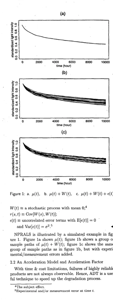
SHIAU/LIN: ANALYZING ACCELERATED DEGRADATION DATA BY NONPARAMETRIC REGRESSION - 151 0 2000 4000 6000 8000 10000 time (hour) 8 0 1 I - 0 2000 4000 6000 8000 10000 time (hour)

(c)

0 2000 - 4000 6000 8000 10000 time (hour) Figure 1: a. p ( t ) , b. p ( t )

+

W ( t ) ,

c. p ( t )

+

W ( t )

+

~ ( t )

W ( t )

=

a stochastic process with mean O;4

~ ( t )

r ( s , t ) Z E Cov[W(s), W ( t ) ] ;

uncorrelated error terms with

E [ E ( ~ ) ]

= 0 ’

and Var[~(t)] = (T’.~ 4

NPRALS is illustrated by a simulated example in fig- ure 1. Figure l a shows p ( t ) ; figure l b shows a group of sample paths of p ( t )

+

W ( t ) ; figure IC shows the same group of sample paths as in figure l b , but with experi- mental/measurement errors added.

2.2 An Acceleration Model and Acceleration Factor With time & cost limitations, failures of highly reliable products are not always observa.ble. Hence, ADT is a use- ful technique to speed up the degradation process.

4The subject effect.

5Experimental and/or measurement error at time t .

Assumptions

rate, not the shape of the degradation curve.

3. The acceleration stress affects only the degradation

4

- - - _

- - - - _

-

c ._ 0 9 1

I

I

0 ‘ 5 10 15 20 25 30 t at

Figure 2: p ( t ) (solid) and p ( a .

t )

(dashed), for some

a

>

1 Figure 2 illustrates assumption #3. The solid curve is

p ( t ) . The dashed curve is p ( a .

t ) ,

where a is the accelera- tion factor. The usual baseline (unaccelerated) process for defining the acceleration factor is the usual-use process; thus usually

a

> 1 for an accelerated process. The same

value of the quality characteristic is observed at,

t

for the accelerated curve,

-

t’

= a .

t

for the unaccelerated curve.

Thus the lifetime

-

defined as the time the degrada- tion path crosses a specified degradation level - of the

accelerated-test item is the lifetime of the product under usual use divided by

a.

Consequently, investigation of the relationship between the SL and the acceleration factors, results in the mean lifetime of highly reliable products un- der usual use. This model is called the scale accelerated failure time (SAFT) model in [lo].

The form of the acceleration time in assumption #3 is

a special kind of acceleration model that might not be adequate to describe the effect of the accelerating variable on time for some problems. See, for example, [9: chapter 181 for other models.

2.3 An Accelerated Life-Stress Degradation Model There are m SL in the experiments. For

SL

i, 1zt ex-

perimental units are used. The product characteristic is measured at t l ,

.

. .

,

t,

for each experimental unit. Using the functional P C technique, consider the accelerated life- stress degradation model in (2) to describe data:

Thus the random component of (l),

W(t)+E(t),

is modeled by a random combination of functional PC,

152 IEEE TRANSACTIONS ON RELIABILITY, VOL. 48, NO. 2, 1999 JUNE

2 ,

3. ESTIMATION

OF

THE MODEL COMPONENTS This section presents an algorithm for estimating p(.)

and a1

,

. . . ,

a,.

These

a,

are not estimable since we do not have data from the unaccelerated process (usual use). We choose the group with the largest acceleration factor as the baseline process. The reason for this choice is that we then can use all the data points in the analysis in the pooling step of the algorithm. Then without loss of generality, let

0

5

a1

5 . .. 5

a ,

= 1. After scaling, the

a,

are no longer acceleration factors. In this section, they are called 'relative acceleration factors'.

Estimate a,, for each

i

= 1,

. . . ,

m,

by solving the mini- mization problem:

r n ;

1

(3)

bm(a,

.

t )

is an estimate of p , ( t ) , for

i

= 1,.

. . ,

m.

Es-

timates of p,(.) and

{a,,

i = 1,.

. . ,

m } are obtained as follows.

{ X m , j , k , j = 1,.

. .

,n,, k =

I,.

. .

, p } on

{ t m , l , k , j = 1 , .

. .

,n,, k = 1 , . . . , p } to obtain an initial

estimate of p m ( . ) . This step can be done more efficiently by smoothing

{ x m , k , k = 1,.

. .

, p } on

1. Smooth

{ t m , j , k , k = 1,.

. .

, p } ,

The derivation is given in the appendix.

2. To estimate a,, search over (0,l) to find the minimizer of (3); this estimate is 6 % .

3. Since all p z ( . ) are just time-scaled functions of p,(.), pool all the data points in m groups together t o estimate p,(.). The data are compiled by mapping each data point

( t w , k , x w , k ) to ( t : , j , k , X 2 ' , j , k ) r

a2

am

&,k E t k ' (T), x,',j,k = X z , j , k .

4. Then obtain

fi,(.)

by smoothing

{ X ~ , 3 r k ,

i

= 1,. . . , m , j = 1,.

.

. , n 2 , k = l , . .

.

, p } on

{ t : , j , k ,

i

=

I,..

.

, m , j = 1 , .

. .

,n,, k = 1,.

.

.

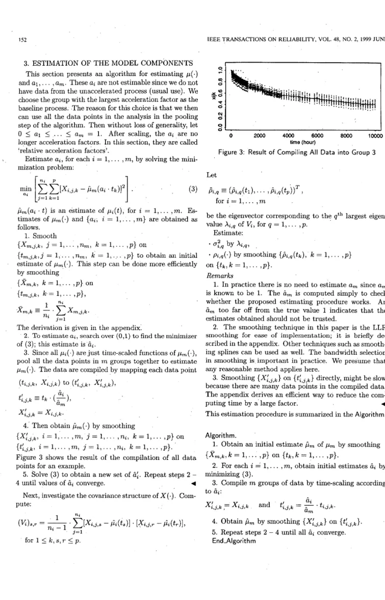
, p } .

Figure 3 shows the result of the compilation of all data points for an example.

5. Solve (3) to obtain a new set of 6:. Repeat steps 2 - 4

Next, investigate the covariance structure of X ( . ) . Com-

4 until values of 6, converge. pute: ni for 1

5

k , s, r

5

p . Let P t , q E ( i j z , q ( t l ) ,

. . .

1 i j z , q ( t p ) ) T

,

f o r i = 1,

...

, m

be the eigenvector corresponding to the qth largest eigen- value A,,q of

V,,

for q = 1,.

. .

, p .

Estimate: * ,:a by x z , q ,

' pz,q(') by smoothing { / % , q ( t k ) , 1,.

. .

,P}

on { t k , k = 1 , .

. .

, p } . Remarks

1. In practice there is no need t o estimate a , since a,

is known to be 1. The 6 , is computed simply to check whether the proposed estimating procedure works. An

6, too far off from the true value 1 indicates that the estimates obtained should not be trusted.

2. The smoothing technique in this paper is the LLR smoothing for ease of implementation; it is briefly de-

scribed in the appendix. Other techniques such as smooth- ing splines can be used as well. The bandwidth selection in smoothing is important in practice. We presume that any reasonable method applies here.

on { t : , l , k } directly, might be slow because there are many data points in the compiled data. The appendix derives an efficient way to reduce the com-

4

This estimation procedure is summarized in the Algorithm.

3. Smoothing

puting time by a large factor.

Algori t h m

.

1. Obtain an initial estimate f i m of p, by smoothing

2. For each

i

= 1,.

. . ,

m,

obtain initial estimates by

3. Compile

m

groups of data by time-scaling according

{ X m , k ,

k

= 1 , .

.

.

, p } On { t k , k = 1,.

. .

, p } . minimizing ( 3 ) . to 6i: X : , j , k

,=

X i , + 6i

t!

z , j , k . =

-

6,

.

t .

2,Jpk. and

4. Obtain

fi,

by smoothing { X i , j , k } on { t i , j , k } .

5.

Repeat steps 2 - 4 until all 6i converge.

SHIAWLIN: ANALYZING ACCELERATED DEGRADATION DATA BY NONPARAMETRIC REGRESSION 153

4. REAL-DATA ANALYSIS

The Algorithm is demonstrated by analyzing a set of real ADT data of an LED product. Items of an LED product were randomly selected for this ADT experiment. The experiment was conducted up to 9998 hours for each

SL.

The key quality characteristic is the SLI which degrades over time. This quality characteristic was measured at 59 time points for each test item. Thus a response curve was collected for each test item.

The accelerating variable is temperature. Three levels

of temperature, 25"C, 65"C, 105OC, were chosen by engi- neers. The usual use condition is 20°C.

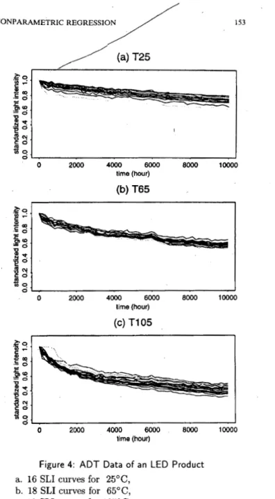
The goal is to estimate the MTTF of the product a t the usual use condition. The 16, 18, 19 response curves were collected for the accelerated conditions, 25"C, 65"C, 105"C, respectively. Figure 4 shows the data. The step- by-step data analysis is shown.

1. The fastest degrading group is group #3 in figure 4c. Let a3 = 1. Apply the Algorithm:

61 = 0.116726, 62 = 0.353575, 63 = 0.999995.

b3

( t ) .

2. Estimate the mean curves of group #1 by

bl(t)

= b 3

.

(2

.

t )

and that of'group #2 by

b 2 ( t ) = b3

.

(2

.

t ) .

To see how well the estimation is, compare

fi,,

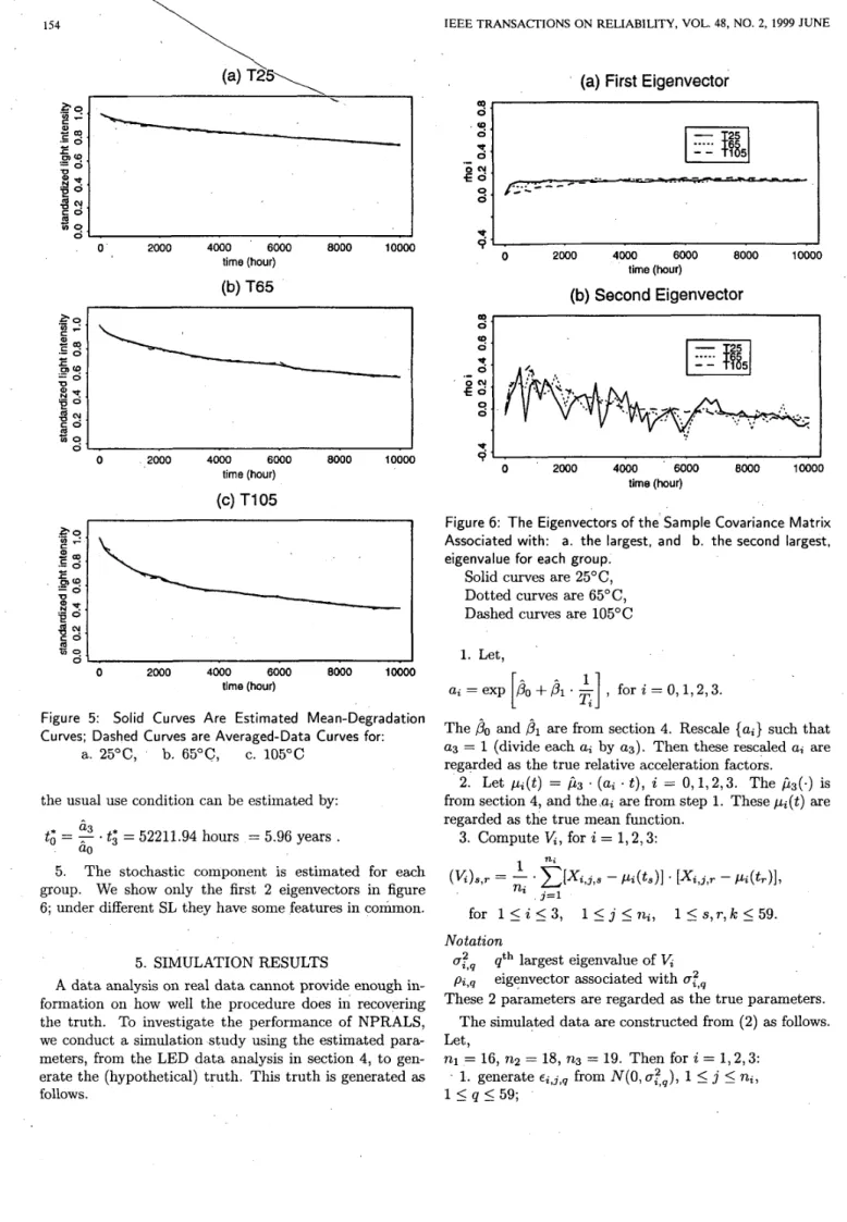
z = 1 , 2 , 3 , with the corresponding averaged curve obtained by aver- aging n, curve data at each of the 59 time points for each group. The results are in figure 5.

Figure 5 shows that:

b,

fits the averaged-curve

i

quite well.

3. Let a0 be the relative acceleration factor under the usual use condition (20°C). To estimate ao, consider find- ing a regression relationship between

{a,}

and the corre- sponding

SL

{T,}. According to [ll], consider the follow- ing Arrhenius rate relationship:

(4)

1

log ( M , ) = a0

+

a1 .

-.

Tz

The Arrhenius relationship [9, 111, obtained through em- pirical observation6, is widely used to describe the effect that temperature has on acceleration. Of course, the con- stant activation-energy does not apply to all temperature- acceleration problems; it is adequate over only a limited temperature range depending on the application. Under the SAFT model, M3/M, =

a,.

Then by (4), it is reason- able that the relative acceleration factor and the SL have the linear relationship:

1

log(ai) = Po

+

P1

.

F , ₍₅₎

si

for some real numbers

PO

and

PI.

Regressing

{&}

on

{1/z}

using model (5), gives $0 = 7.9438 and $1 .= 61n principle, it merely defines t h e activation energy.

I50 0 2000 4000 6000 BOO0 IO000 time (hour)

(b)

T65 i 0 2000 4000 6000 8000 10000 time (hour)

(c)

T105

1 I 0 2000 4000 6000 BOO0 10000 time (hour)

Figure 4: A D T Data of an LED Product

a. 16 SLI curves for 25"C, b. 18 SLI curves for 65"C, c. 19 SLI curves for 105°C

-3017.0264. P-values for $0 _{and are less than 0.05,}

and

R2

=O .9975.

These evidences support the potential adequacy of (5).

Further, since the usual use condition (20°C) is not too far away from the temperature range tested, we then can estimate the relative acceleration factor at the usual use condition by

"

]

= 0.09559846.

60 = exp

[-

PO

+

273.16

+

20

4. By an industrial standard, an LED product is de- clared failed when its SLI degrades to 1/2. Consequently, we can estimate the MTTF of the LED product in group

154 IEEE TRANSACTIONS ON RELIABILITY, VOL. 48, NO. 2, 1999 JUNE 2000 4000 6000 8000 10000 time (hour)

(b)

T65 O , 0 Zoo0 4000 6000 8000 10000 time (hour)

(c) T105

0 2000 4000 6000 EO00 loo00 time (hour)

Figure 5: Solid Curves Are Estimated Mean-Degradation Curves; Dashed Curves are Averaged-Data Curves for:

a. 25"C, b. 65"C, c. 105°C

the usual use condition can be estimated by:

k 3

t;

=

tz

= 52211.94 hours = 5.96 years

.

5. The stochastic component is estimated for each group. We show only the first 2 eigenvectors in figure

6; under different SL they have some features in common.

a0

5. SIMULATION RESULTS

A data analysis on real data cannot provide enough in- formation on how well the procedure does in recovering the truth. To investigate the performance of NPRALS, we conduct a simulation study using the estimated para- meters, from the LED data analysis in section 4, to gen- erate the (hypothetical) truth. This truth is generated

as

follows. 0 2000 4000 6000 8000 10000 time (hour)

(b)

Second Eigenvector

01 I I ' 0 2000 4000 6000 8000 10000 time (hour)

Figure 6: The Eigenvectors o f t h e Sample Covariance Matrix Associated with: a. the largest, and b. the second largest, eigenvalue for each group.

Solid curves are 25"C,

Dotted curves are 65"C,

Dashed curves are 105°C 1. Let,

ai = exp 0 0

+

,&

The

00

and 81are from section 4. Rescale { a i } such that

a3 = 1 (divide each ai by a s ) . Then these rescaled ai are

regarded as the true relative acceleration factors.

2. Let p i ( t ) = f i 3 . (ai

.

t ) , i

= 0 , 1 , 2 , 3 . The f i 3 ( . ) is

from section 4, and the,ai are from step 1. These p i ( t ) are regarded as the true mean function.

3. Compute

V,, for

i

= 1 , 2 , 3 :

,

for

i

= 0 , 1 , 2 , 3 .

[-

4

for 1 5 i 5 3 , 1 5 j 5 n i , 1 < s , r , k 5 5 9 .

Notation

u ; , ~ qth largest eigenvalue of ~ l ,

pi,q eigenvector associated with u : , ~

These 2 parameters are regarded

as

the true parameters. The simulated data are constructed from (2) as follows. Let,

n1 = 16, n2 = 18, 723 = 19. Then for

i

= 1 , 2 , 3 : . 1. generate ~ i , j , ~ from N(O,U?,), 1

5

j

5

ni,

~

SHIAU/LIN: ANALYZING ACCELERATED DEGRADATION DATA BY NONPARAMETRIC REGRESSION 155

(a)

T25

0 2000 4000 6000 8000 10000 time (hour)

(b)

T65

z

" X

I

0 2000 4000 6000 8000 10000 time (hour)

(c)

T105

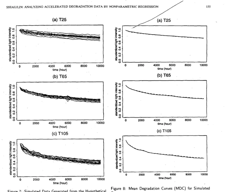
I 0 2000 4000 6000 8000 10000 time (hour)

Figure 7: Simulated Data Generated from the Hypothetical True Model

a. 16 SLI curves for 25"C,

b. 18

SLI

curves for 65"C, c. 19 SLI curves for 105°C

Figure 7 shows the generated data; these simulated data have many features of the real data.

Perform the procedure, described in section 3, on the simulated data { X i , j ; k } . The estimates of

ai

are summa- rized in table 1.

-

Figure 8 shows f i i ( . ) and the hypothetical true mean curves. 0 2000 4000 6000 8000 10000 time (hour)

(b) T65

0 2000 4000 6000 8000 10000 time (hour) (c)

T105

4000 6000 EO00 10000 0 2000 lime (hour)

Figure 8 : Mean Degradation Curves (MDC) for Simulated Data

Dashed curves: estimated MDC Solid curves: (hypothetical) true MDC

a. 25"C, b. 65"C, c. 105°C

-

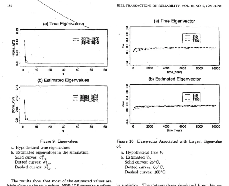
Figure 9 shows c ; , ~ , the'hypothetical true eigenvalues, and &;,q, the estimated eigenvalues.

-

Figures 10, 11 show the hypothetical true and the es- timated eigenvectors associated with the largest and the second-largest eigenvalues, respectively.

Table 1: True & Estimated Values of the ai

a0 a1 a2 a3

True 0.09559894 0.1175793 0.3891789 1 Est. 0.09052029 0.1063360 0.3987680 0.999993

(a) True Eigenv3-

0 10 20 30 40 50 6 q

(b) Estimated Eigenvalues

" I

& 0 1

I

- -

1

L . I 0 10 , 20 30 40 50 60 q Figure 9: Eigenvalues

a. Hypothetical true eigenvalues

b. Estimated eigenvalues in the simulation. Solid curves: (T:,~,

Dotted curves: (T; 9 ,

Dashed curves: mi,,

The results show that most of the estimated values are fairly close to the true values. NPRALS seems to perform quite well for this simulated example. This also indicates that NPRALS describes the LED data fairly well.

6. DISCUSSION

Meeker, Escobar, Lu [lo] presented some good meth- ods, based on- parametric models, for analyzing acceler- ated degradation data similar to the data analyzed in this paper.

A

nonparametric regression alternative, such

as

NPRALS can free analysts from the burden of specifying models in the usual parametric modeling. The tradeoff is the slight inefficiency, which means one probably needs more data to get the same accuracy of the estimates using a parametric model (assuming that the parametric model is correct). On the other hand, a nonparametric regression method performs much better than a wrongly specified parametric model. A popular data-analysis strategy is to explore the data via nonparametric regression techniques first; if the results suggest a suitable parametric model, then perform the usual parametric methods for:

-

better efficiency,

-

possibly easier interpretation.

Nonparametric regression is a fast growing research area

IEEE TRANSACTIONS ON RELIABILITY, VOL. 48, NO. 2, 1999 JUNE

(a) True Eigenvector

'1

0

. .

0 2000 4000 6000 8000 10000 time (hour)

(b)

Estimated Eigenvector

0 1

I

2

01 6 1 I 0 2000 4000 6OOO 8000' 10000 time (hour)

Figure 10: Eigenvector Associated with Largest Eigenvalue

Of: a. Hypothetical true

V ,

b. Estimated

V,.

Solid curves: 25"C, Dotted curves: 65"C, Dashed curves: 105°C

in statistics. The data-analyses developed from this re-

search are getting more mature and advanced. The poten- tial applications of these techniques are in any area that needs regression techniques, such as the application in this paper.

In this paper, the goal of estimating MTTF for the LED product under usual use is achieved by finding the relation- ship between the relative acceleration factors and the

SL.

The important issues

of

obtaining

an

interval estimate of MTTF and estimating the lifetime distribution are topics for future research.

ACKNOWLEDGMENT

We are pleased to thank the editor, an 'zsociate editor, two anonymous referees, and Prof. Sheng-Tsaing Tseng of National Tsing Hua University, whose helpful suggestions led to a great improvement on the quality of the paper. We are very grateful to Prof. Tseng for providing the LED data to us. Jyh-Jen Shiau is grateful t o the Department of Statistics at Stanford University for their hospitality; this paper was revised during her visit there. This research was partially supported by the National Science Council of the Republic of China, Grant No. NSC88-2118-M-009-009.

SHIAU/LIN: ANAL.YZING ACCELERATED DEGRADATION DATA BY NONPARAMETRIC REGRESSION

/

157

(a)

True Eigenvector

(0

1

0 - T 91

I

0 2000 , 4000 6000 8000 10000 time (hour)

(b) Estimated

Eigenvector

W

1

0 -

*

~ ' 0 2000 4000 6000 8000 10000 time (hour)

h = the bandwidth ST the local smoothing.

b(t)

is explicJt1.y

i'

expressed by,

For this study, we chose Epanechnikov kernel for

IT(.):

K ( t )

=

9

.

(1

-

t 2 )

.

I(ltl

5

1).

Epanechnikov kernel is one of the most popular kernels in nonparametric regression; it is the optimal kernel in the sense that it minimizes asymptotic mean squared error of the function estimator over a group of kernels [2: theorem

3.41. For more information on LLR smoothers, see, eg, [2, 4 , 51.

A.2 Method Extension

Figure 11: Eigenvector Associated with Second-Largest Eigenvalue o f

For group

m,

the LLR estimator of P m ( t )

n- P a. Hypothetical true V , b. Estimated Vi. . Solid curves: 25"C, Dotted curves: 65"C, Dashed curves: 105°C APPENDIX

Appendix A . l briefly describes the LLR smoother method to smoothing one curve data. Appendix A.2' ex- tends the method to estimating efficiently the mean curve of a group of curve data. Appendix A.3 further extends the method to estimating efficiently the mean curve from the complied data of several groups of curve data.

A.

1 Local Linear Regression Smoother

This is a locally weighted least squares estimation. Given n observations

{

( t k , y k ) } ; = l

,

consider the model:

Y k = P ( t k )

+

E k , k = 1,.

. . ,

7 2 ,

for 1 = 1 , 2 , n = nm ' p .

nm

Xm,k E x X m , j , k ,

j = 1

Since w,,j7k = wm,jt,k, for all j , j ' = 1 , . .

.

, n m , then by

setting Wm,k = wm,j,k,

P P

wm,k ' Xm,k wm,k ' x m , k

p ( , ) is a smooth function

{ f k } are uncorrelated errors with zero mean and standard

We obtain a b(t) by the minimizer

min c ( y k - bo - bl(tk

-

t)12

.

Kh(tk -

t )

,

k = l - - k=l deviation D . b m ( t ) = P P nm ' Wm,k Wm,k of k=l k=l

Thus, smoothing all the data

{ X m , j , k i j = 1 , .

. .

, n m ,

k

= 1 , .

. .

,P}

can be simplified to smoothing

bo'b1 k = l

r

1

1

h

Kh(.) z? -

.

K

(;)

.

-

IEEE TRANSACTIONS, ON RELIABILITY, VOL. 48, NO. 2, 1999 JUNE

A.3 Further Method Extension

mator of p m ( t ) is:

For

the compiled data

m n; P m n; P i = l j=1 k=l

I

= 1,2,

n =

( n l +

...

+ n m ) ‘ p . Notation n; w i , k w i , j , k

Since W i , j , k = w i , j ( , k , for all j , j ’ = 1,

.

. .

,

n;,

m p m p

i = l k=l

m. Q

i=l k=l

Thus, smoothing all the data:

i = 1,.

. .

,m, j = 1 , .

. . ,

ni,

IC = 1 , .

. .

, p } can

be simplified to smoothing:

{Xl,k2

-

i = 1 , .

. .

,

m, IC = 1 , .

. .

, p } with adjusted weights

On {xL,k}. 4

REFERENCES

W.B. Capra, H.-G. Muller, “An accelerated-time model for response curves”, J. Amencan Statwtacal Assoc, vol

92, 1997 Mar, pp 72 - 83.

J. Fan, I. Gijbels, Local Polynomaal Modelang and

Its

Ap- plzcatzons, 1996; Chapman & Hall.

P.J. Green, B. W. Silverman, Nonpammetnc Regressaon

and Generalzzed Lanear Model. A Roughness Penalty Ap- proach, 1994; Chapman & Hall.

W. Hardle, Applzed Nonpararnetnc Regressaon, 1990;

Cambridge Univ. Press.

[5] W. Hardle, Smoothing Techniques: With Implementation in S, 1991; Springer-Verlag.

[6] T. Hastie, R. Tibshirani, Generalized Additive Models,

1990; Chapman & Hall. ’

[7] C.J. Lu, W.Q. Meeker, “Using degradation measures to es- timate a time-to-failure distribution”, Technometrics, vol

35, 1993 May, pp 161 - 174.

[8] W.Q. Meeker, L.A. Escobar, “A review of recent research and current issues in accelerated testing”, Znt’l Statistical

Review, vol 61, 1993 Apr, pp 147 - 168.

[9] W.Q. Meeker, L.A. Escobar, Reliability Data Analysis,

1998; John Wiley & Sons.

[lo] W.Q. Meeker, L.A. Escobar, C.J. Lu, “Accelerated degra- dation tests: Modeling and analysis”, Technometrics, vol 40, 1998 May, pp 89 - 99.

(111

W.

Nelson, Accelerated Testing: Statistical Models, Test

Plans, and Data Analysis, 1990; John Wiley & Sons.

[12] J.O. Ramsey, B.W. Silverman, finctional Data Analysis,

1997; Springer.

[13] G. Wahba, Spline Models for Observational Data, 1990;

Society for Industrial and Applied Mathematics.

(141 H.F. Yu, S.T. Tseng, “On-line procedure for terminating an accelerated degradation test”, Statistica Sinica, vol 8, 1998 Apr, pp 207 - 220.

AUTHORS

Dr. Jyh-Jen Horng Shiau; Institute of Statistics; National Chiao Tung Univ.; Hsinchu 300 TAIWAN - R.O.C.

Internet (e-mail): jyhjen@stat.nctu.edu.tw

Jyh-Jen Horng Shiau received her BS in Mathematics from the National Taiwan University, MS in Applied Mathe- matics from the University of Maryland Baltimore County, MS in Computer Science and PhD in Statistics from the Univer- sity of Wisconsin - Madison. She taught in Southern Methodist University, University of Missouri at Columbia, and National Tsing Hua University, and worked for Engineering Research Center of AT&T Bell Labs before she moved to Hsinchu, Taiwan, where she is an Associate Professor in the Insti- tute of Statistics at the National Chiao Tung University. Her interests include industrial statistics and nonparametric func- tion estimation. She is a member of Institute of Mathematical Statistics .

Hsin-Hua Lin; Institute of Statistics; National Chiao Tung Univ.; Hsinchu 300 TAIWAN

-

R.O.C.

Hsin-Hua Lin is a graduate student in the Institute of Sta- tistics at the National Chiao Tung University. She received her

BS in Mathematics from Chung Yuan Christian University. She is interested in industrial statistics.

Manuscript TR1998-136 received: 1998 September 8;

revised: 1998 October 7, 1999 February 23

Responsible editor: H.-K. Hsieh