Clustering Time Series Data by SOM for the Optimal Hedge Ratio Estimation
Yu-Chia Hsu
1 2, An-Pin Chen
11
Institute of Information Management, National Chiao Tung University, Taiwan,
2Mackay Medicine, Nursing and Management College, Taiwan
[email protected], [email protected]
Abstract
The fat-tailed and leptokurtic properties observed in most financial asset return series would cause the inaccuracy of hedge ratio estimation because most traditional statistics approaches are based on the assumption of normal distribution. In this study, a novel approach is proposed using self-organizing map (SOM, also called Kohonen’s Self-Organizing Feature Map) for time series data clustering and similar pattern recognition to improve the optimal hedge ratio (OHR) estimation. Five SOM-based models (considering the weight for averaging and the interval for data sampling) and two traditional models (ordinary least square method and naïve hedge) were compared in Taiwan stock market hedging. The experiment demonstrates the feasibility of applying SOM, and the empirical results show that SOM approach provides a useful alternative to the OHR estimation.
1. Introduction
The futures market is one of the most important aspects of the financial market. In 2007, the total trading volume of global futures and options reached 15 billion US dollars; this growth rate has accelerated since then [1]. Many investors consider the futures market as a powerful risk management tool because it can provide hedging, speculation, arbitrage, and price discovery functions. On the other hand, it is helpful in increasing market efficiency and integrity.
As a risk management tool, hedging has become an important issue. Many conditions should be determined when hedging: hedge target, hedge horizon, hedge ratio, and other like conditions. In general, the hedge target is chosen according to the correlation between the spot and futures, and the hedge horizon is determined by the hedger’s subjective identity. Traditionally, the appropriate hedge ratio can be estimated by the ordinary least square (OLS)
method or the mean-variance model. The OHR is commonly defined as the hedge ratio under the minimal risk with specific risk aversion. But these models are time invariant and cannot reflect the dynamic behaviour of the time series. Recently, studies have applied econometrics models (e.g., GARCH family models) to estimate the OHR in empirical studies which suggest that the OHR has the time variant and the hedged portfolio needs to be adjusted frequently during the hedge horizon [3] [4].
Nevertheless, these financial models, which are based on the assumption that the investors’ behaviour is completely rational and the financial markets are efficient and have been challenged since the emergence of such financial behaviour in the last three decades. In other words, the return series of the financial asset does not fit the normal distribution [5]; on the contrary, most of them are fat-tailed or leptokurtic. Therefore, the hedge ratio estimation based on the OLS and mean-variance (MV) models have poor accuracy, theoretically. Moreover, additional conditions such as risk aversion and utility function are hard to be estimated. The expected payoff is assumed marginable, and the return series of different trading day is independent, hence causing the inaccuracy of the OHR estimation.
The GARCH family models are capable of catching the dynamic behaviour of the financial time series and have been widely used for forecasting volatility and for estimating portfolio risk. However, these models have several drawbacks when dealing with time series forecasting. One of the drawbacks shows that the models require the time series to be stationary; thus, the price series of a financial asset is usually transformed to the return series by differential. It will, nonetheless, eliminate much information and ignore the property such as the co-integrated. Consequently, studies have tried to improve the GARCH family models by adding the error term or other variables to the models. Such improvement can increase accuracy, but the models, together with other variables, becomes more and more complicated. Another drawback is
Third 2008 International Conference on Convergence and Hybrid Information Technology Third 2008 International Conference on Convergence and Hybrid Information Technology Third 2008 International Conference on Convergence and Hybrid Information Technology
shown in the data sampling frequency. Most empirical studies adopt the same sampling frequency for estimation and forecasting periods. For example, the hedge ratio in the next five days is determined according to data with five-day sampling frequency; the hedge ratio in the next three weeks is determined according to the data with three-week sampling frequency. These models cannot work when dealing with different sampling frequencies; the information and property of the original time series may be eliminated after data sampling [6]. Nonetheless, while certain studies are devoted to the improvement of the GARCH models [7] [11], others propose to simply alternate approaches based on the moving average [8].
Another issue is the hedge strategy, which can be classified as static and dynamic hedge. In order to avoid transaction cost, the static hedge strategy suggests that the hedge portfolio should not be changed frequently during the hedge horizon. The natural property of the financial time series, however, is dynamically changing. Studies suggest that the hedger should consider time-variant hedge ratio in order to obtain better hedge effeteness. As a result, the dynamic hedge strategy stands that the hedge portfolio should be adjusted more frequently according to the latest estimated hedge ratio until the hedge horizon is due.
In this study, we propose the new hedge ratio estimating approach using SOM which serves as an unsupervised two-layered network that can organize a topological map. The resulting map shows the natural relationships among the patterns that are given to the network. SOM is suitable for clustering analysis and has been applied to time series forecasting [9] [10]. However, the feasibility of using SOM to deal with the variance and covariance of time series forecasting has not been studied.
The research process is described as follows. First, the time series are clustered with SOM. Second, the hedge ratio is calculated based on the cluster of the similarity time series pattern. We assume that the similar time series pattern will have the same behaviour and will be suitable for hedge ratio estimation. Finally, several SOM-based models we propose are investigated and compared with the traditional models using the rolling window approach in out-sample testing. The experiment results can provide a valuable reference for adopting the SOM approach without considering too many assumptions and restrictions in previous models.
The rest of the paper is organized as follows: Section 2 illustrates the basic model for the OHR estimation; Section 3 details the research method; Section 4 analyzes the experiment results; and lastly, Section 5 draws conclusions from the study.
2. Estimation of the Optimal Hedge Ratio
2.1 Minimum Variance Hedging
Minimum variance hedging is the most important concept of portfolio risk management. Investors hold the spot position and futures position at the same time to compose the portfolio. The risk of the portfolio is usually measured by the variance. Consequently, hedging with the minimum risk hedge ratio is also called minimum variance hedging. For a long position in the spot market, the return hedged portfolio is given by F h S HP=Δ − Δ Δ (1)
where h is the hedge ratio. SΔ and FΔ are the changes in the spot and futures prices, respectively. The price change can also be represented as the return, which is continuously compounded and defined as ln(Pt/Pt−1) multiplied by 100.
The OHR is the value of h that maximizes the investor’s expected utility. When the futures price follows a martingale, the expected futures return is zero; therefore, the futures position will not affect the expected return of the portfolio. The OHR is simply the value of h that minimizes the variance of equation (1) which is given by 0 2 2 ) var( , 2 − = = ∂ Δ ∂ Δ Δ ΔF S F h h HP σ σ (2) where 2 F Δ
σ is the variance of the futures return and
F S Δ Δ ,
σ is the covariance between the spot return and
the futures return. The OHR is determined by solving equation (2): 2 , * F F S h Δ Δ Δ = σ σ (3)
The OHR given by equation (3) can be estimated by regressing the spot return on the futures return using OLS. This approach is also viewed as the conventional OHR. Equation (3) also considers the conditioning on recent information for more efficient estimate of the OHR. The most commonly used practice is the rolling window approach, where the variance and covariance of the spot and futures are estimated at time t according to the conditioning on the time t-1 information set.
The degree of hedging effeteness is measured by the percentage reduction in the variance of portfolio after hedging. Therefore, the hedge effectiveness (HE) can be noted as ) var( ) var( 1 2 2 2 S HP HE unhedged hedged hedged un Δ Δ − = − = − σ σ σ (4)
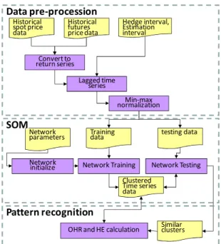
Traditional OLS hedge ratio is estimated on the regressing spot return on the futures return under the assumption that the probability distribution of the spot and futures return series come from normal distribution. However, most financial asset returns do not follow the assumption; hence, the variance and covariance estimated by OLS is inaccurate. Consequently, we propose that the variance and covariance should be estimated using similar time series data. SOM clustered historical time series data with similar patterns. The perfect hedge ratio, such that the HE equation (4) equals to 1, can be calculated in advance. Therefore, when the hedge ratio for next hedge horizon is estimated, we can refer to the known hedge ratio in the past with similar time series pattern. A corresponding flow chart of the proposed scheme is shown in Figure 1. Network parameters Historical spot price data Network initialize Convert to return series
OHR and HE calculation Historical futures price data Lagged time series Min-max normalization Training
data testing data
Network Training Hedge interval, Estimation interval Clustered Time series data Network Testing Data pre-procession SOM Similar clusters Pattern recognition
Figure 1. The SOM approach for OHR estimation The OHR estimating procedure involves five steps:
(a) SOM initialization. The appropriate parameters of the SOM are determined: network topology, number of the neuron in the input layer, radius of the near area, learning rate, among others.
(b) Data pre-procession. The input variables for time series pattern recognition and similarity search are verified; the lagged time series is calculated; and the input value between -1 and 1 is normalized. (c) Network training. A vector composed of the
historical time series is entered into the SOM. The output of a neuron is established by calculating a similar measure between the weight of that neuron and the external input using the competitive learning, which is widely used in machine learning.
(d) Similar pattern recognition. In testing period, the trained SOM can select the similar days in the historical time series for OHR estimation.
(e) OHR calculation. The OHR is estimated using the OLS hedge ratio of the similar clustered time series data.
3. Research Method
3.1 Constructing the SOM Model
The feasibility of using SOM to estimate the OHR is examined through the five SOM-based models that we propose. Generally, the hedge ratio implies the relationship of the spot and futures price change degree. Many empirical studies indicate the existence of the co-integration relations between spot and futures prices; the co-integration relations would be eliminated when mapping the price series to the return series. Furthermore, the basis between the spot and futures prices is helpful for estimating the hedge ratio [2]. Therefore, we adopt the two series, the spot price series and the basis series, as the input variables of SOM model. The SOM model can be expressed as follows:
] , ,.., [ 1 S t S t S e t S t p p p P = − − (5) ] , ,.., [ tFe tF1 tF F t p p p P = − − (6) F t S t F S t P P B , = − (7) ) , ( S,F t S t k F P B N = (8) where S t P , F t
P are the spots and futures price series
with e days lag before current day, respectively. SF t
B , is the basis series derived from the spot and futures prices. F is the function representing the SOM. Nk is the output of the SOM, representing the numbers of the clustered time series data.
The SOM model for OHR estimation is designed on two basic concepts: one, to calculate the average OHR of the clustered data; and two, to calculate the OHR using the data in different intervals.
Let Et and Eˆt denote the clustered data sets. S t
Pˆ
and F
t
Pˆ are the price series in the f days ahead hedge
intervals } , { F t S t t P P E = (9) ] .., , [ ˆ 2 1 S f t S t S t S t p p p P = + + + (10) ] , .., , [ ˆ 2 1 tF tFf F t F t p p p P = + + + (11) } ˆ , ˆ { ˆ F t S t t P P E = (12) Five different SOM-based OHRs are estimated by equations (13) to (18):
∑
∑
= = = m i i m i i TWA SOM d h d OHR i 1 1 _ 1 1 (13) where t F F S i E h t t t ˆ 2 Δ Δ Δ =σσ (14) 2. Equal-weighted average 1 _ _ = = d OHROHRSOM EWA SOM EWA (15)
3. Estimation interval t F F S EI SOM E OHR t t t 2 _ Δ Δ Δ = σ σ (16) 4. Hedge interval t F F S HI SOM E OHR t t t ˆ 2 _ Δ Δ Δ = σ σ (17)
5. Estimation and hedging intervals
} ˆ , { 2 _ t t F F S EH SOM E E OHR t t t Δ Δ Δ = σ σ (18)
3.2 Data and Experiment Design
This study obtains the empirical trading data of the daily closing price of the Taiwan weighted index (Taiwan Stock Exchange and the Taiwan Index Futures traded on the Taiwan Futures Exchange, AREMOS database). The futures prices series was gathered from the nearest month contracts and rolled over to the next nearest contracts on the maturity day due to the consideration of liquidity and price spread risk. The data were selected from 2 January 2003 to 14 July 2008. After clearing the irregular data, a total of 1,300 observations are used for experiments.
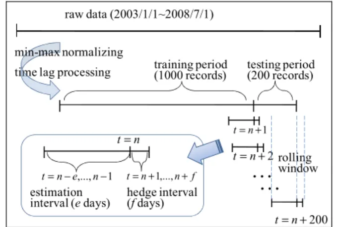
After operating for e days lag and f days ahead in equations (5) ~ (12), the data are divided into two parts. The first 1,000 records are used for SOM in-sample training, and the last 200 records are used for out-sample testing. A rolling window scheme is designed for dynamic hedge ratio estimation, as illustrated in Figure 2. The rolling windows are expected to roll 200 times to test the 200 out-sample data for each experiment.
raw data (2003/1/1~2008/7/1)
time lag processing training period(1000 records) testing period(200 records) min-max normalizing
…
200 + = n t 1 + = n t 2 + = n t 1 ,..., − − =n e n t t=n+1,...,n+f n t= estimationinterval (e days) hedge interval (f days)
rolling window
…
Figure 2. Rolling windowWe assume that the hedged portfolio is adjusted every f days; this is the hedged interval. The hedge effectiveness is calculated at the end of the hedge interval on the (t+f) -th day using equation (4). In order to reflect the real hedge effectiveness during the hedge interval, we use equation (10) and (11) to obtain the hedge effectiveness.
The experiments are designed to investigate the feasibility of SOM for OHR estimation. Therefore, the value of the main parameters and variables used in the SOM model are tested, including the numbers of nodes in the SOM topology, the numbers of days in the estimation interval, and the number of days of the hedge interval. A total of 72 experiments are performed in this study according to the different parameters listed in Table 1. In addition, for each experiment performed 200 times for dynamic hedge using rolling window, we use the average of the OHR and HE for evaluating.
The SOM models we proposed are also compared with two traditional methods: the OLS hedge and the naïve hedge. The OLS hedge ratio is calculated with the sampled data from the 1,000 records in the SOM training period. For example, if the hedge interval is one week, we use the weekly data gathered in the training period to estimate the OLS hedge ratio. Moreover, the OLS hedge effectiveness is calculated according to the SOM models using the daily data of the following week.
Table 1. Parameters setting of the experiments
Parameter Unit Value
Number of SOM nodes Nodes 22, 32, 42
Estimation interval (e) Days 7, 14, 21, 28 Hedge interval (f) Days 3, 5, 7, 14, 21, 28
4. Experiment Results
The appropriate parameter setting of the SOM models we proposed is one of the key interests in this
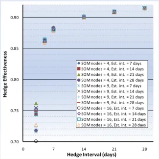
study. Figure 3 illustrates the hedge effectiveness under different parameter settings for estimating the time-weighted average OHR. Figure 3 clearly shows that the estimation interval and the number of SOM nodes are not sensitive to the HE under the same hedge interval, except when the hedge interval is three days. In addition, the HE increases when the hedge interval increases. 0.70 0.75 0.80 0.85 0.90 0 7 14 21 28 H edge E ff ec ti v ene ss
Hedge Interval (days)
SOM nodes = 4, Est. int. = 7 days SOM nodes = 4, Est. int. = 14 days SOM nodes = 4, Est. int. = 21 days SOM nodes = 4, Est. int. = 28 days SOM nodes = 9, Est. int. = 7 days SOM nodes = 9, Est. int. = 14 days SOM nodes = 9, Est. int. = 21 days SOM nodes = 9, Est. int. = 28 days SOM nodes = 16, Est. int. = 7 days SOM nodes = 16, Est. int. = 14 days SOM nodes = 16, Est. int. = 21 days SOM nodes = 16, Est. int. = 28 days
Figure 3. HE distribution in various conditions To understand the differences among the modes in testing period, we pick one of the experiments and detail the results in Figures 4, 5, and 6. The experiment we picked is performed when the number of SOM nodes, the estimation interval, and the hedge interval are set to 4 days, 7 days, and 7 days, respectively.
In Figure 4, the spot and futures prices are very close. However, a market downturn occurs from 23 July 2007 to 3 September 2007; the basis becomes more positive. Meanwhile, the OHR and HE in Figures 5 and 6 are not particular with other periods. When the market upturn occurs as shown in Figure 5 between 14 June 2007 and 19 September 2007, the HE in Figure 6 becomes worst. Figure 5 also shows the OHR of the time-weighted average SOM model is the smallest most of the time. Moreover, the OHR of OLS model seems to vibrate periodically.
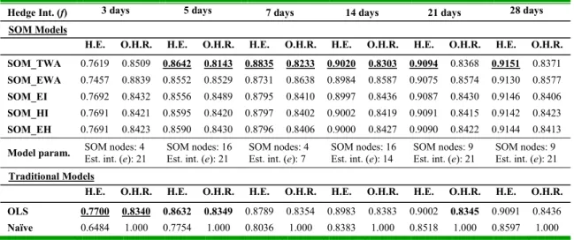
For the next step, we compare the five proposed SOM models with the two traditional models. The HE value represents the degree of the risk reduction; the value of OHR refers to the hedge cost. Consequently, the model with high HE and low OHR value is excellent. The different parameter settings of SOM models lead to approximate experiment results in the same hedge interval. Only the six best outcomes are
selected according to the SOM-TWA-HE of the 72 experiments and are listed in Table 2 for comparison.
7000 7500 8000 8500 9000 9500 10000 2007/1/19 2007/3/13 2007/4/25 2007/6/7 2007/7/23 2007/9/3 2007/10/18 D ai ly c lo sin g p ric e
Taiwan weighted index Taiwan Index Futures
Figure 4. Out-sample testing data
0.70 0.75 0.80 0.85 0.90 0.95 1.00 1 51 101 151 Hed ge R at io
SOM_TWA SOM_EWA SOM_EI SOM_HI SOM_EH OLS Naïve
Figure 5. OHR in the testing period
-0.10 0.00 0.10 0.20 0.30 0.40 0.50 0.60 0.70 0.80 0.90 1.00 1 51 101 151 Hed ge E ffect iv en es s
SOM_TWA SOM_EWA SOM_EI SOM_HI SOM_EH OLS Naïve
Figure 6. Hedge Effectiveness in the testing period When the hedge interval is three days, the traditional OLS model has the best HE and OHR. In the five days hedge interval, the OLS model’s HE can also beat the SOM models, besides the SOM_TWA. The HE and OHR of the five SOM models are very close, with the SOM_TWA model as the best among them. The naïve model is the worst in all hedge intervals within our expectation.
5. Conclusion and Future Work
This study uses SOM to cluster the time series data and also uses the similarity clustered data for the OHR estimation. The empirical results briefly show the outcomes of the proposed models, as compared with the traditional models. The SOM approaches can have a little improvement to hedge effectiveness, with the smaller hedge ratio being helpful in decreasing hedge cost. Furthermore, when the hedge horizon is
increased, the hedge effectiveness is also increased. These results indicate that the setting of the parameters in SOM models is not sensitive to hedge effectiveness. Consequently, the model parameters estimation procedure can be avoided. In the future, the SOM model may be used to verify the strength of other markets. Finally, we suggest that other information derived from the time series (e.g., the technique indicators or the filter banks) be used for data clustering to improve the SOM model.
Table 2. Model comparison
Hedge Int. (f) 3 days 5 days 7 days 14 days 21 days 28 days SOM Models
H.E. O.H.R. H.E. O.H.R. H.E. O.H.R. H.E. O.H.R. H.E. O.H.R. H.E. O.H.R. SOM_TWA 0.7619 0.8509 0.8642 0.8143 0.8835 0.8233 0.9020 0.8303 0.9094 0.8368 0.9151 0.8371
SOM_EWA 0.7457 0.8839 0.8552 0.8529 0.8731 0.8638 0.8984 0.8587 0.9075 0.8574 0.9130 0.8577
SOM_EI 0.7692 0.8432 0.8556 0.8489 0.8795 0.8410 0.8997 0.8436 0.9087 0.8430 0.9146 0.8406
SOM_HI 0.7691 0.8421 0.8595 0.8420 0.8797 0.8402 0.9002 0.8419 0.9091 0.8415 0.9142 0.8423
SOM_EH 0.7691 0.8423 0.8590 0.8430 0.8796 0.8406 0.9000 0.8427 0.9090 0.8422 0.9144 0.8413
Model param. SOM nodes: 4 Est. int. (e): 21 SOM nodes: 16 Est. int. (e): 21 SOM nodes: 4 Est. int. (e): 7 SOM nodes: 16 Est. int. (e): 14 SOM nodes: 9 Est. int. (e): 21 SOM nodes: 9 Est. int. (e): 21 Traditional Models
H.E. O.H.R. H.E. O.H.R. H.E. O.H.R. H.E. O.H.R. H.E. O.H.R. H.E. O.H.R. OLS 0.7700 0.8340 0.8632 0.8349 0.8789 0.8354 0.8983 0.8383 0.9002 0.8345 0.9091 0.8436 Naïve 0.6484 1.000 0.7754 1.000 0.8036 1.000 0.8383 1.000 0.8518 1.000 0.8597 1.000
6. References
[1] Galen Burghardt, “Volume Surges Again: Global Futures and Options Trading Rises 28% in 2007”, Futures Industry Magazine, Mar/Apr, 2008, pp. 14-26.
[2] Donald D. Lien and Li Yang, “ Spot-Futures Spread ,Time-varying Correlation, and Hedging With Currency Futures”, Journal of Futures Market, Vol. 26, 2006, pp.1019-1038.
[3] K. F. Kroner, J. Sultan., “Time-Varying Distributions and Dynamic Hedging with. Foreign Currency Futures”, Journal of Finance and Quantitative analysis, Vol. 28, No. 4, 1993, pp. 535-551.
[4] Taufiq Choudhry, “Short-run deviations and optimal hedge ratio: evidence from stock futures”, Journal of Multinational Financial Management, Vol. 13, issue 2, 2003, pp. 171-192.
[5] Bollerslev, T., R. Chou, and K. Kroner, “ARCH modeling in finance: A review of the theory and empirical evidence,” Journal of Econometrics, Vol. 52, 1992, pp.5-59. [6] Keshab Man Shrestha and Donald Lien, “An Empirical Analysis of the Relationship between the Hedge Ratio and Hedging Horizon Using Wavelet Analysis,” Journal of Futures Markets, Vol. 27, No. 2, 2007, pp. 127-150.
[7] Robert F. Engle, “Dynamic Conditional Correlation: A Simple Class of Multivariate Generalized Autoregressive Conditional Heteroskedasticity Model”, Journal of Business and Economic Statistics, Vol. 20, issue 3, 2002, pp. 339-350. [8] Brooks, C., & Chong, J. “The cross-currency hedging performance of implied versus statistical forecasting models”, Journal of Futures Markets, Vol. 21, 2001, pp. 1043-1069.
[9] Senjyu, T. Tamaki, Y. and Uezato, K., “Next day load curve forecasting using self organizing map”, Proceedings of the International Conference on Power System Technology 2000, vol.2, 2000, pp. 1113-1118.
[10] Mark O. Afolabi and Olatoyosi Olude, “Predicting Stock Prices Using a Hybrid Kohonen Self Organizing Map (SOM)”, Proceedings of the 40th Annual Hawaii International Conference on System Sciences, 2007, pp.48. [11] Ghysels, E., Santa-Clara, P. and R. Valkanov, “Predicting Volatility: How to Get theMost Out of Returns Data Sampled at Different Frequencies,” Journal of Econometrics, Vol. 131, 2006, pp. 59-95.