台灣證券市場上從眾行為與市場及橫斷面報酬率間關係之研究(第2年)

科技部補助專題研究計畫成果報告

期末報告

台灣證券市場上從眾行為與市場及橫斷面報酬率間關係之研究

(第2年)

中　華　民　國　105　年　10　月　11　日

中 文 摘 要 ： 在這個兩年期計畫的第二年計畫中，我們檢驗市場從眾行為如何影 響台灣股市的橫斷面報酬。我們首先依標準化後之估計貝它值將每 個月的橫斷面報酬率區分為十個投資組合，並發現這些投資組合的 平均報酬率不僅跟估計貝它值的大小沒有單調關係，也似乎並不隨 著市場從眾程度的大小而變化。這似乎反映出台灣股市的淺碟型特 徵。透過迴歸分析，我們也並未發現高低貝它投資組合之間的報酬 差異會顯著受到市場從眾程度大小的影響。與Hwang and Salmon (2009)的研究結果相較，市場從眾行為影響台灣股市的方式與其對 美國股市之影響並不相同。

中 文 關 鍵 詞 ： 從眾；反從眾；資產定價異常。

英 文 摘 要 ： This is the second year‘s report of a two-year project. In this follow-up

project, we investigate how market herding behavior may affect cross-sectional asset returns on Taiwan‘s stock market. We first form decile portfolios according to

standardized beta, and find that beta does not forecast the following month’s cross-sectional returns neither

unconditionally, nor conditional on the market herding state.

This seems to reflect the shallow-disk characteristics of Taiwan‘s security market, where individual traders are easily infected by noises or attention-grabbing events. The regression analysis results also show that the high minus low beta returns are not significantly affected by the lagged market herding measure, which indicates that there hasn‘t been any asset pricing anomaly created by market herding behavior on Taiwan‘s stock market. Unlike the study of Hwang and Salmon (2009), the impact of market herding behavior on cross-sectional

asset returns on the Taiwanese security market is different from that on the U.S.

Herding and Returns on Taiwan’s Stock Market

(Second Year)

Shinn-Juh Lin

Department of International Business

National Chengchi University

October 10, 2016

Abstract

This is the second year’s report of a two-year project. In this follow-up project, we investigate how market herding behavior may affect cross-sectional asset returns on Taiwan’s stock market. We first form decile portfolios according to standardized beta, and find that beta does not forecast the following months cross-sectional returns neither unconditionally, nor conditional on the market herding state. This seems to reflect the shallow-disk characteristics of Taiwan’s security market, where individual traders are easily infected by noises or attention-grabbing events. The regression analysis results also show that the high minus low beta returns are not significantly affected by the lagged market herding measure, which indicates that there hasn’t been any asset pricing anomaly created by market herding behavior on Taiwan’s stock market. Unlike the study of Hwang and Salmon (2009), the impact of market herding behavior on cross-sectional asset returns on the Taiwanese security market is different from that on the U.S.

JEL Classification: G11; G12; G14.

1

Introduction

This is the second year’s report of a two-year project. In this follow-up project, we inves-tigate how market herding behavior may affect cross-sectional asset returns on Taiwan’s stock market.

In the first year, we applied Hwang and Salmon’s (2009) beta herding measure to examine empirical properties of herding on Taiwan’s stock market, and its relationship with market sentiment. We find time-varying beta herding behavior on Taiwan’s stock market. Interestingly, irrespective of the factor model used in estimating these herding measure, the degree of herding are higher in the pre-2000 period (with Asian financial crisis and the Dot-com bubble), and the post-2008 period (the Great Recession). Our regression results also support the fact that beta herding exhibits a negative relationship with sentiment. This is different from the U.S. evidence found in Hwang and Salmon (2009) which states that herding does not occur when financial markets are in stress (or in crisis). Presumably, this is because Taiwan’s stock market is more dominated by noise-traders. Furthermore, with the quantile regression analyses, we have found that a higher beta herding measure (smaller degree of market herding) can significantly and positively affect market returns in their left tail distribution (below the 20th _{quantile of the market}

return distribution.) In other words, during market downturns, a higher degree of market herding can aggravate the panic of the market and investors, which then causes the market return to drop even further.

In short, Our first year’s results clearly indicate that returns on Taiwan’s security market may also be affected by herding behavior (also evidenced by Lo and Li, 2009; Yeh, and Li, 2012.) In addition, it has been well documented that beta does not fully explain cross-sectional asset returns, e.g., Fama and French (1992, 1993, 1996). It is interesting to know how herding behavior may affect cross-sectional asset returns. Therefore, in this

follow-up project, we intend to investigate how herding behavior may affect cross-sectional asset returns, and hence create some asset pricing anomaly on Taiwan’s stock market. The idea is that, during periods with high degree of market herding, more investors tend to make investment decisions based on movements on the market rather than follow their own beliefs and information. Consequently, the supposedly differential performance of stocks with large and small betas becomes insignificant. In contrast, during periods with low degree of market herding, investor’s beliefs and information are incorporated into investment decision, difference between large and small betas may then imply differential performance of stocks.

To proceed with such investigation, we first form decile portfolios according to stan-dardized beta, and examine how relative performance of such deciles portfolios might be affected by the degree of market herding. For a more detailed analysis, we further examine such relations in a regression framework, where differentials in returns between high and low beta portfolios are regress on the beta herding measure and other control variables, such as size, value-growth, and momentum factors

To summarize, with decile portfolios formed according to standardized beta, we find that beta does not forecast the following months cross-sectional returns neither uncondi-tionally, nor conditional on the market herding state. This seems to reflect the shallow-disk characteristics of Taiwan’s security market, where individual traders are easily infected by noises or attention-grabbing events. The regression analysis results also show that the high minus low beta returns are not significantly affected by the lagged market herd-ing measure, which indicates that there hasn’t been any asset pricherd-ing anomaly created by market herding behavior on Taiwan’s stock market. Unlike the study of Hwang and Salmon (2009), the impact of market herding behavior on cross-sectional asset returns on the Taiwanese security market is different from that on the U.S.

The rest of the paper is organized as follows. Section 2 describes sample data used 2

in this project. Section 3 provides an update on the herding measure estimates with an extended sample period. Section 4 outlines the methodology employed in this second year project. Section 5 presents and discusses the empirical results obtained. I conclude this report in Section 6.

2

Data

Our sample period consists of 308 monthly observations of all common stocks traded on the Taiwan stock exchange, with financial firms excluded, from January 1991 to August 2016. The number of stocks starts from 213 at January 1996 and increases to 1266 at August 2016. For computing excess returns, the average one-month time deposit rate from five main Taiwanese commercial bank is used to proxy the risk-free rate. Together with returns on the mimicking portfolio for the size factor (SMB), the value-growth factor (HML), the momentum factor (MOM), and all other required data are retrieved from the Taiwan Economic Journal (TEJ).

3

Update on the Herding Measure Estimates

Although stock markets worldwide have, to some extent, recovered from the financial crisis of 2007-08, it is widely believed the global economy is still struggling with slow growth, so is investors’ confidence in financial markets. Presumably, as part of the global financial market, Taiwan’s security market is yet to recover from the financial crisis, either. To offer an update of research findings in our first year’s project, we extend our sample period from 1991/01∼2012/12 to 1991/01∼2016/08, and examine whether market herding behavior has changed in the entire post-2008 period.

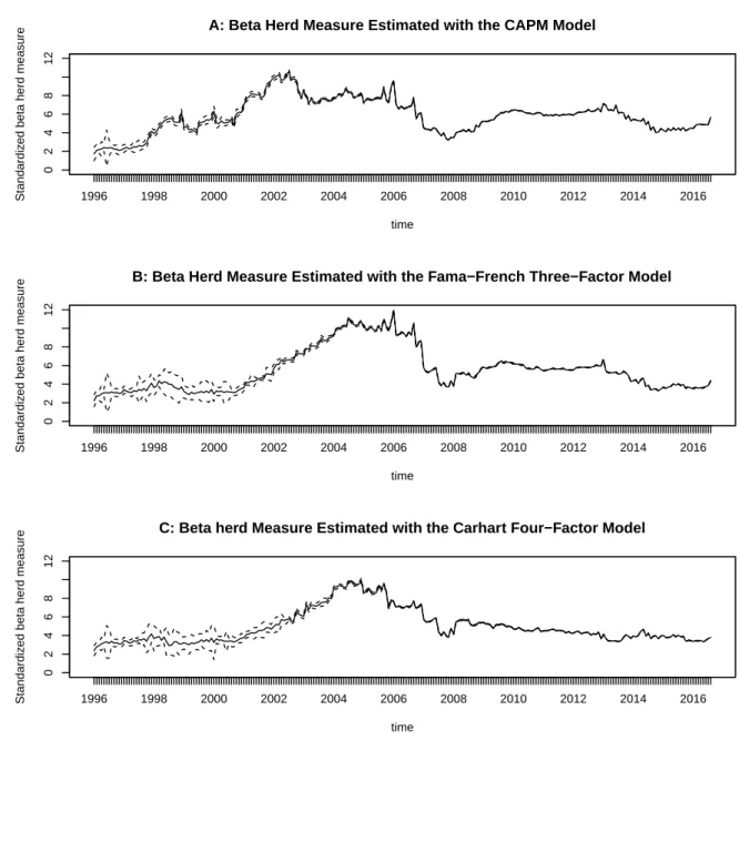
Figure 1 shows the updated version of the evolution of market herding (estimated with three factor models: the CAPM model, the Fama-French threefactor model and Carhart four-factor model) over time (1996/01∼2016/08) on Taiwan’s stock market with 95% confidence interval represented by the dashed lines.1 _{Although the confidence band} may seem large before year 2000 when a relatively small number of stocks are traded on the market, it has significantly reduced to a very small region with hundreds more of new stocks traded on the Taiwan stock exchange, so that we observe many significant but small changes in herding activity.

It is interesting to note that, irrespective of the factor model used in estimating these herding measure, the degree of herding are higher (with smaller beta herding values) in the pre-2000 period (with Asian financial crisis and the Dot-com bubble), and the post-2008 period (the Great Recession). Such pattern is more pronounced when the beta herding measures are estimated with the Fama-French threefactor model and Carhart four-factor model. This is different from the U.S. evidence found in Hwang and Salmon (2009), which states that herding does not occur when financial markets are in stress (or in crisis). Presumably, this is because Taiwan’s stock market is more dominated by

noise-1_{Since the previous 60 months of data are required to estimate the betas from asset pricing models,}

our market herding estimates only start from 1996/01.

Figure 1: Evolution of herding over time on Taiwan’s stock market 1996 1998 2000 2002 2004 2006 2008 2010 2012 2014 2016 0 2 4 6 8 12 time Standardiz

ed beta herd measure

A: Beta Herd Measure Estimated with the CAPM Model

1996 1998 2000 2002 2004 2006 2008 2010 2012 2014 2016 0 2 4 6 8 12 time Standardiz

ed beta herd measure

B: Beta Herd Measure Estimated with the Fama−French Three−Factor Model

1996 1998 2000 2002 2004 2006 2008 2010 2012 2014 2016 0 2 4 6 8 12 time Standardiz

ed beta herd measure

C: Beta herd Measure Estimated with the Carhart Four−Factor Model

traders. It is most interesting to note that 8 years after the financial crisis of 2007-08, the degree of market herding (the market herding measure) has remained at a relatively high (low) level. In particular, such a trend has not changed since 2012. This provides further evidence of the shallow-disk characteristics of Taiwan’s security market, where individual traders are easily infected by noises or attention-grabbing events.

4

Methodology

To prepare for the ensuing tests, we first form decile portfolios, for each month, sorted on standardized betas, ( bβs imt− β s mt ) /σ_bβs imt, where β s mt ≡ 1 N N ∑ i=1

βs_imt is the cross-sectional average of the beta estimate, βs_imt.2 _{Then, for each of these portfolios formed in month t,} we calculate the following month’s (t + 1) equally weighted return.

For an exploratory view of how cross-sessional returns may be affected by market herding, decile portfolios formed above are then grouped into one of three herding states in the previous month, namely, herding (bottom 30% of herd measure), no herding (middle 40% of herd measure) and adverse herding (top 30% of herd measure.) Comparison of return differentials of decile portfolios among these three herding states then offers a crude view of the impact from market herding.

Furthermore, in order to specifically test if the cross-sectional return difference between high and low beta herding portfolios changes significantly depending on the level of beta herding, we run the following regressions

rβ_high,t+h− rβ_low,t+h= γ₀+ γ₁H_mt∗ + εi,t+h, (1)

and

rβ_high,t+h− r_low,t+hβ = γ₀+ γ₁H_mt∗ + γ₂SM Bt+h+ γ3HM L + γ4M OM + εi,t+h. (2)

The high and low beta portfolio returns, rβ_high,t+h and r_low,t+hβ are obtained by equally weighting the top and bottom 30% of stocks formed on the standardized betas. Equation (2) controls for impacts from the size, value-growth and the momentum factors. Note that we omit excess market return from the right-hand side since the regressand is the

2_{Since weights attached to individual stocks in forming the market portfolio are not equal, E(β}s

imt)̸= 1,

we use the cross-sectional sample mean of the beta estimates, βs_mt, in place of the population mean of β,

E(βs_imt), to compute the standardized beta.

beta-sorted portfolio returns. We also set h = 1, 3, 6, 9, and 12 in order to investigate the explanatory power of beta herding on the beta sorted portfolios over time. For h > 1, we follow Jegadeesh and Titman (2001) and construct overlapping portfolios to increase the power of the tests. For instance, rβ_high,t+h is calculated by equally weighting h high beta portfolios formed at t, t + 1, . . . , t + h− 1.

Presumably, during periods with high degree of market herding (low H_mt∗ value), more investors tend to make investment decisions based on movements on the market rather than follow their own beliefs and information. Consequently, the supposedly differential performance of stocks with large and small betas becomes insignificant. In contrast, during periods with low degree of market herding (high H_mt∗ value), investor’s beliefs and information are incorporated into investment decision, difference between large and small betas may then imply differential performance of stocks. Henceforth, we expected the coefficient, γ₁, on the lagged beat herding measure, H_mt∗ , to be positive.

5

Empirical Results

5.1

An Exploratory View

In Table 1, we report an exploratory view of how portfolio returns may be affected by beta and market herding state.

[Insert Table 1 about here]

The first row of Panel A, B, and C in Table 1 confirms that, as in Fama and French (1992, 1993,1996), beta in Taiwans equity market does not forecast the following months cross-sectional returns unconditionally. In Hwang and Salmon’s (2009) study, they find that, after being conditioned on the herding level, high beta stocks tend to show higher returns after adverse herding for the U.S. equity market. However, we do not observe the same pattern for the Taiwanese market, as indicated in the following three rows of Panel A, B, and C in Table 1. In other words, returns of the standardized beta sorted portfolios do not necessarily increase with the standardized betas following an adverse herding state, nor do they decrease following a herding state. This, again, seems to reflect the shallow-disk characteristics of Taiwan’s security market, where individual traders are easily infected by noises or attention-grabbing events. As presented in Figure 1, a whole chunk of our sample period (typically post-crisis period) are followed by higher degree of market herding. This offers a possible explanation why we do not observe similar empirical patter as those presented in Hwang and Salmon (2009). However, we do find an interesting regularity. That is, from the last rows of Panel A, B, and C in Table 1, that returns are typically higher following an adverse herding state than those following a herding state for both high and low beta portfolios. In other words, investors have been able to make higher returns out their own beliefs and information in non-herding states.

5.2

Regression Analyses

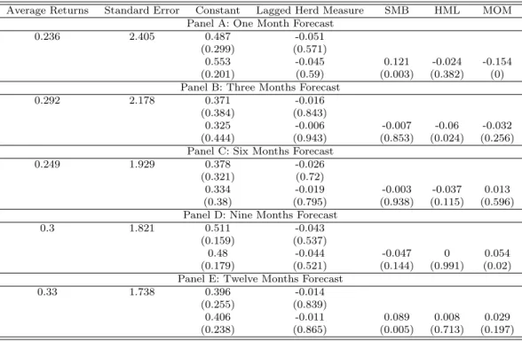
We report regression results of Equation (1) and (2) in Table 2. Note that, unlike the study of Hwang and Salmon (2009), coefficients on the lagged beta herding measure in our regression analyses are all insignificantly negative irrespective of the forecasting horizons, which means the spread between the high and low beta portfolio returns becomes larger with a smaller beta herding measure (higher market herding.) The insignificant results also indicates that there hasn’t been any asset pricing anomaly created by market herding behavior on Taiwan’s stock market.

[Insert Table 2 about here]

To summarize, the impact of market herding behavior on cross-sectional asset returns on the Taiwanese security market is different from that on the U.S. security market, and it has not created an asset pricing anomaly on Taiwan’s stock market.

6

Conclusion

In this second year’s project, we investigate how market herding behavior may affect cross-sectional asset returns on Taiwan’s stock market. We first form decile portfolios according to standardized beta, and find that beta does not forecast the following months cross-sectional returns neither unconditionally, nor conditional on the market herding state. This seems to reflect the shallow-disk characteristics of Taiwan’s security market, where individual traders are easily infected by noises or attention-grabbing events. The regres-sion analysis results also show that the high minus low beta returns are not significantly affected by the lagged market herding measure, which indicates that there hasn’t been any asset pricing anomaly created by market herding behavior on Taiwan’s stock market. Unlike the study of Hwang and Salmon (2009), the impact of market herding behavior on cross-sectional asset returns on the Taiwanese security market is different from that on the U.S.

References

[1] Fama, E. F., and K. R. French, 1992, “The Cross Section of Expected Stock Returns,”

Journal of Finance 47, 427-465.

[2] Fama, E. F., and K. R. French, 1993, ”Common risk factors in the returns on stocks and bonds,” Journal of Financial Economics, 33, 3-56.

[3] Fama, E. F., and K. R. French, 1996, ”Multifactor explanations of asset pricing anoma-lies,” Journal of Finance, 51, 55-84.

[4] Hwang, S. and M. Salmon, “Sentiment and Beta Herding,” March 18, 2009, available at SSRN: http://ssrn.com/abstract=299919 or http://dx.doi.org/10.2139/ssrn.299919. [5] Jegadeesh, Narasimhan and Sheridan Titman, 2001, “Profitability of Momentum

Strategies: An Evaluation of Alternative Explanations,” The Journal of Finance, 56, 699-720.

[6] Lo, Chin-Shui, and Chun-An Li, 2009, “The Impact of Herding and Non-herding on Market Returns,” Management Review 28, 21-41.

[7] Yeh, Chih-Cheng, and Chun-An Li, 2012, “The Relationship Among Investor Sen-timent, Herding and Non-herding,” Review of Securities and Futures Markets, 24:3, 141-182.

T able 1: F uture Returns Conditioning on Herding The table rep orts future returns conditioning on herding states. F or eac h mon th from 1987/01 to 2016/08, w e form decile p ortfolios sorted on standardized b etas and then calculate the follo wing mon th’s equally w eigh ted return for eac h of these p ortfolios, dep ending on the previous mon th’s herding states, i.e., adv erse herding, no herding, and herding, are formed on the top 30%, middle 40%, and b ottom 30% of the herd measures. Results in P anel A, B and C are based on the CAPM Mo del, the F ama-F renc h Three-F actor Mo del, and the Carhart F our-F actor Mo del, resp ectiv ely . P anel A: CAPM Mo del Herding Activit y P1 P2 P3 P4 P5 P6 P7 P8 P9 P10 P10-P1 All 0.734 0.492 0.500 0.371 0.407 0.470 0.110 0.424 0.393 0.297 -0.437 Herding (Bottom 30%) 0.067 -0.443 -0.319 -0.667 -0.305 -0.221 -0.940 -0.143 -0.014 0.037 -0.030 Herding (Middle 40%) 0.876 0.978 0.695 0.932 1.128 1.187 1.102 1.380 1.052 1.045 0.169 Adv erse Herding (T op 30%) 1.214 0.783 1.059 0.664 0.162 0.210 -0.158 -0.276 -0.072 -0.434 -1.648 Adv erse Herding -Herding 1.147 1.226 1.378 1.331 0.467 0.431 0.782 -0.133 -0.058 -0.471 -1.618 P anel B: F ama-F renc h Three-F actor Mo del Herding Activit y P1 P2 P3 P4 P5 P6 P7 P8 P9 P10 P10-P1 All 0.648 0.527 0.612 0.384 0.600 0.284 0.356 0.025 0.549 0.207 -0.441 Herding (Bottom 30%) -0.362 -0.896 -0.630 -0.937 -0.605 -1.538 -1.017 -1.556 -0.396 -1.425 -1.063 Herding (Middle 40%) 0.598 0.722 0.677 0.554 0.619 0.528 0.260 0.229 0.303 0.253 -0.345 Adv erse Herding (T op 30%) 1.724 1.691 1.769 1.479 1.779 1.784 1.855 1.335 1.820 1.776 0.052 Adv erse Herding -Herding 2.086 2.587 2.399 2.416 2.384 3.322 2.872 2.891 2.216 3.201 1.115 P anel C: Carhart F our-F actor Mo del Herding Activit y P1 P2 P3 P4 P5 P6 P7 P8 P9 P10 P10-P1 All 0.570 0.689 0.641 0.225 0.592 0.343 0.285 0.094 0.352 0.277 -0.293 Herding (Bottom 30%) -0.837 -0.539 -0.259 -1.593 -0.553 -1.578 -1.078 -1.514 -1.601 -1.255 -0.418 Herding (Middle 40%) 0.894 1.044 0.658 0.785 0.778 0.928 0.698 0.540 1.144 0.974 0.080 Adv erse Herding (T op 30%) 1.545 1.447 1.518 1.300 1.491 1.490 1.099 1.111 1.254 0.883 -0.662 Adv erse Herding -Herding 2.382 1.986 1.777 2.893 2.044 3.068 2.177 2.625 2.855 2.138 -0.244 14

Table 2: Time Series Regression of High minus Low Beta Portfolio Returns on Lagged Herd Measure & Carhart Four-Factors

In this table, we run the time series regression of high minus low beta portfolio returns on lagged herd measure & Carhart four-factors. The high and low beta portfolio returns, rβ_high,t+hand rβ_low,t+hare obtained by equally weighting the top and bottom 30% of stocks formed on the standardized betas. The second equation controls for impacts from the size, value-growth and the momentum factors. We also set h = 1, 3, 6, 9, and 12 in order to investigate the explanatory power of beta herding on the beta sorted portfolios over time. The numbers in the brackets represent Newey-West robust p−value.

Average Returns Standard Error Constant Lagged Herd Measure SMB HML MOM Panel A: One Month Forecast

0.236 2.405 0.487 -0.051

(0.299) (0.571)

0.553 -0.045 0.121 -0.024 -0.154 (0.201) (0.59) (0.003) (0.382) (0) Panel B: Three Months Forecast

0.292 2.178 0.371 -0.016

(0.384) (0.843)

0.325 -0.006 -0.007 -0.06 -0.032 (0.444) (0.943) (0.853) (0.024) (0.256) Panel C: Six Months Forecast

0.249 1.929 0.378 -0.026

(0.321) (0.72)

0.334 -0.019 -0.003 -0.037 0.013 (0.38) (0.795) (0.938) (0.115) (0.596) Panel D: Nine Months Forecast

0.3 1.821 0.511 -0.043

(0.159) (0.537)

0.48 -0.044 -0.047 0 0.054

(0.179) (0.521) (0.144) (0.991) (0.02) Panel E: Twelve Months Forecast

0.33 1.738 0.396 -0.014

(0.255) (0.839)

0.406 -0.011 0.089 0.008 0.029 (0.238) (0.865) (0.005) (0.713) (0.197)

1

科技部補助專題研究計畫出席國際學術會議心得報告

日期：105 年 07 月 11 日

一、 參加會議經過

本次研討會我被安排在 7 月 1 日的第 166 場次 CONTAGION AND DEPENDENCE session，該場次 共有四位學者發表學術論文。本人發表的論文題目為“Analyzing profitability of momentum

strategies in Taiwan’s stock market”。另外，本人也擔任同場次 “Evaluation of Copula-based

Dependence Structure in the U.S. Agricultural Future Markets”一文之評論工作。除了我自己的報告場 次之外，我也參加了多場次其他學者的演講。另外，我也聽了兩場主題演講，一場是由已獲得 2009 年 John Bates Clark Medal 的經濟學家 Emmanuel Saez 講述有關財富和收入不平等原因方面的前沿 研究：“Income and Wealth Inequality: Evidence and Policy Implications”。他檢視美國和其他國家的收 入-稅收資料，來對收入不平等提供歷史估計；在他們的調查結果中，在金融危機開始前，收入前 1% 的家庭佔有了美國將近四分之一的收入，其最大份額起始於 19 世紀 20 年代後期。另一場則是 由獲得 1995 年 John Bates Clark Medal 的經濟學家 David Card 講述被頂級經濟期刊（QJE, JEEA, ReStud, and Restat）接受刊登的決定性因素："What Gets In? Editorial Decisions at Top Economics Journals"。主要在探討這些頂級經濟期刊的編審過程是否有不公平的現象。

二、與會心得

這次到美國波特蘭參加學術研討會，會中評論人對本篇文章提供了非常多寶貴的建議，讓本篇論 文在將來投稿前，有一個良好的修正依據。除了從其他學者身上得到投稿前論文修改的許多寶貴 建議之外；與其他與會學者之間的研究經驗交流，對於瞭解時下經濟財務主要研究問題的了解與 釐清都有相當不錯的幫助；另外，聆聽兩位已經獲得 John Bates Clark Medal 經濟學家的主題演講，

計畫編號

MOST

103-2410-H-004-034-MY2

計畫名稱

出國人員

姓名

林信助

服務機構

及職稱

會議時間

會議地點

Hilton Portland & Executive Tower,

Oregon

會議名稱

(中文) 國際西方經濟學會第 91 屆年會

(英文) WEAI 91st Annual Conference

發表題目

(中文) 台灣股市動能交易策略獲利性之分析

(英文) Analyzing profitability of momentum strategies in Taiwan’s stock

market

2

對於當前學術頂尖前沿研究的理解，也有很大的助益。

二、 發表論文全文或摘要

This paper examines six momentum strategies in Taiwan’s stock market. These include the price-, the industry-, the 52-week high-, the moving average ratio-, the residual-, and the earnings-momentum strategies, which have all been popular in studies of the American and the European stock markets. We examine respective profitability of those six momentum strategies, and compare their relative strength. Our empirical results show that the 52-week high-, the residual-, and the earnings-momentum strategies generate significantly positive profit, with the profit of the 52-week high being the highest. In addition, the 52-week high- and the earnings-momentum strategies both provide additional explanatory power to returns conditional on the other four momentum strategies. On the contrary, the other four momentum strategies do not offer additional explanatory power to returns conditional on the 52-week high- or the earnings-momentum strategies. Furthermore, following George and Hwang’s (2004) regression model, we conduct a composite analysis of the six momentum strategies, and find that the profitability of the 52-week high momentum strategy is significantly better than other strategies. Overall, the 52-week high-momentum strategy stands out as the most profitable momentum indicator in Taiwan’s stock

四、建議

五、攜回資料名稱及內容

六、其他

Analyzing profitability of momentum strategies in Taiwan’s

stock market

Kuan-Cheng Ko

Department of Banking and Finance, National Chi Nan University

Shinn-Juh Lin*

Department of International Business, National Chengchi University

Chien-Wei Peng

Department of Banking and Finance, National Chi Nan University

June 10, 2016

Abstract

This paper examines six momentum strategies in Taiwan’s stock market. These include the price-, the industry-, the 52-week high-, the moving average ratio-, the residual-, and the

earnings-momentum strategies, which have all been popular in studies of the American and the European stock markets. We examine respective profitability of those six momentum strategies, and compare their relative strength. Our empirical results show that the 52-week high-, the residual-, and the earnings-momentum strategies generate significantly positive profit, with the profit of the 52-week high being the highest. In addition, the 52-week high- and the

earnings-momentum strategies both provide additional explanatory power to returns conditional on the other four momentum strategies. On the contrary, the other four momentum strategies do not offer additional explanatory power to returns conditional on the 52-week high- or the earnings-momentum strategies. Furthermore, following George and Hwang’s (2004) regression model, we conduct a composite analysis of the six momentum strategies, and find that the profitability of the 52-week high momentum strategy is significantly better than other strategies. Overall, the 52-week high-momentum strategy stands out as the most profitable momentum indicator in Taiwan’s stock market.

Keywords: Price momentum; Industry momentum; 52-week high; Moving average ratio;

Residual momentum; Earnings momentum

* _{Corresponding author: Dr. Shinn-Juh Lin at 64, SEC. 2, Tz-Nan Rd., Wenshan, Taipei 116, Taiwan. Tel.: + 886 2} 29393091x81106; fax: + 886 2 29387699, email: [email protected].

  2

1

Introduction

On security market, it is typical to observe stock prices that have been increasing in the past keep increasing in the short to intermediate future, and hence produce the so-called

momentum effect. Jegadeesh and Titman (1993) document that firms with high returns over the past three months to one year continue to outperform firms with low past returns over the same period. Since then, researchers have attempted to examine such momentum effect from different perspectives. Moskowitz and Grinblatt (1999) show that individual stock momentum is largely driven by industry momentum, and that stocks within the same industry tend to be more highly correlated than stocks across industries. George and Hwang (2004) find that the 52-week high price explains a large portion of the profits from momentum investing. Park (2010) proposes that investors’ anchoring bias by using the moving averages or the 52-week high as reference points for estimating fundamental values is the primary source of

momentum effects. He finds that the moving average ratio (MAR, ratio of short-term moving average to the long-term moving average) combined with nearness to the 52-week high explains most of the intermediate-term momentum profits. Blitz, Huij and Martens (2011) argue that conventional momentum strategies exhibit substantial time-varying exposures to the Fama and French factors. They propose a residual momentum strategy which is based on residual returns estimated using the Fama and French three-factor model. By examining the profitability of residual momentum strategy using the all U.S. domestic data that covers the period from January 1926 to December 2009, they find that the residual momentum strategy succeeds in improving upon a total return momentum strategy of Jegadeesh and Titman (1993, 2001). Chan, Jegadeesh and Lakonishok (1996) find that medium-term return continuation can be explained in part by under-reaction to earnings information. They show that earnings

  3

momentum strategies are profitable even among larger stocks and that the profitability cannot be explained by the Fama-French three-factor model. To summarize, the price-, the industry-, the 52-week high-, the moving average ratio-, the residual- and the earnings- momentum are the six most often examined momentum strategies.

In Taiwan’s stock market, profitability of the price-, the earnings-, the industry- and the 52-week high moment strategies have been separately examined, while the MAR- and the residual momentum strategies have not received due attention in the literature. Intriguingly, these studies have not demonstrated unambiguous results regarding profitability of each momentum strategy. More importantly, there has not been a comprehensive study nor

comparison of profitability of popular moment strategies in Taiwan’s stock market. Therefore, by employing data of common stocks listed on the Taiwan Stock Exchange from January 1981 to December 2010, this paper proposes to thoroughly examine profitability of all those six popular momentum strategies with different holding periods. With pairwise comparison, we compare profitability of momentum strategies in pairs. Furthermore, we follow regression model of George and Hwang (2004) to to ascertain whether profitability of a particular momentum strategy is significantly better than others. As robustness checks, we also examine whether our empirical results are affected by the January effect, different lengths of the portfolio formation period, and different market states (bull or bear markets).

Overall, our empirical results show that the 52-week high-, the residual-, and the earnings-momentum strategies generate significantly positive profit, with the 52-week high-momentum strategy stands out as the most profitable momentum indicator in Taiwan’s stock market. With different lengths of portfolio formation period, we find that a price momentum portfolio formed according to the past 6 month returns can produce significant

  4

positive profit, which is consistent with findings in Jegadeesh and Titman (1993). However, the industry momentum portfolios show no significant profit. In addition, the 52-week high- and earnings-momentum strategies both provide additional explanatory power to returns conditional on the other four momentum strategies. On the contrary, the other four momentum strategies do not offer additional explanatory power to returns conditional on the 52-week high- or the earnings-momentum strategies. Furthermore, following George and Hwang’s (2004) regression model, we also conduct a composite analysis of the six momentum strategies, and find that the profitability of the 52-week high momentum strategy is

significantly better than other strategies. In robustness tests, our empirical results show that returns to losers portfolio become much smaller after January months are excluded, and result in even higher momentum profit. This indicates that the January effect does have a

significant effect on momentum profitability. Furthermore, the profitability of the 52-week high-momentum strategy is not affected by different lengths of portfolio formation period, and different market states.

The rest of this paper is organized as follows. In Section 2, we describe the data used in this paper. Construction of various residual momentum strategies and our research

methodologies are introduced in Section 3. Section 4 presents empirical results with robustness checks. The last section offers concluding remarks.

2

Data Description

Our sample consists of returns and firm characteristics of all common stocks listed on the Taiwan Stock Exchange (TWSE) from January 1981 to December 2010. The data are

retrieved from the Taiwan Economic Journal (TEJ), which is a local data vendor in Taiwan. Financial firms and firms with negative book values are excluded from our sample.

  5

Continuously compound returns,R , are calculated as _t

, P P ln = R 1 t-t t (1)

whereP is the closing price at time t. Industry portfolios are constructed according to the 28 _t

industry groups designed by the TWSE.2 _{Within each industry, returns are weighted by} market values of component stocks. For residual momentum strategy, the Fama and French (1993) three-factor model is employed to computed residual returns. Following Fama and French (1992), a firm's book-to-market equity for July of year t to June of year t + 1 is

calculated as the book value of fiscal year t − 1, divided by market equity at the end of

calendar year t − 1.

3

Methodology

3.1 Construction of Momentum Strategy Indicators

Momentum strategies examined in this paper include the price momentum strategy of Jegadeesh and Titman (1993) (JT hereafter), the industry momentum strategy of Moskowitz and Grinblatt (1999) (MG hereafter), the 52-week high momentum strategy of George and Hwang (2004) (H52 hereafter), the moving average ratio momentum strategy of Park (2010) (MAR hereafter), the residual momentum strategy of Blitz, Huij and Martens (2011) (RS hereafter), and the earnings momentum strategy of Chan, Jegadeesh and Lakonishok (1996) (Earn hereafter). In the following, we briefly outline the construction of the indicator for each momentum strategy in sequence.

2 _{According to the TWSE, individual stocks are grouped into the following categories: Cement, Foods, Plastics,}

Textiles, Electric Machinery, Electrical and Cable, Glass & Ceramics, Paper & Pulp, Iron and Steel, Rubber, Automobile, Building Material and Construction, Shipping and Transportation, Tourism, Finance and Insurance, Trading and Consumers' Goods, Chemical, Biotechnology and Medical Care, Oil, Gas and Electricity, Semiconductor, Computer and Peripheral Equipment, Optoelectronics, Communications and Internet, Electronic Parts & Components, Electronic Products Distribution, Information Service, Other Electronics, and Others,

  6

1. The JT momentum strategy：

Following Jegadeesh and Titman (1993), the JT momentum strategy indicator is constructed based on average returns of the past twelve months as follows

12 , 1 , 1: 12 ₁₂ , i t j j i t t R R     



where R_i,t represents return of stock i at month t; whileR_i,t1:t-12 represents average return of

stock i during the past twelve months.

2. The MG momentum strategy：

Following Moskowitz and Grinblatt (1999), the MG momentum strategy indicator is constructed based on average returns of each industrial group during the past twelve months as follows, 12 , 1 , 1: -12 ₁₂ , i t j j i t t IR IR    



whereIR represents return of industrial group i at month t; while_it, IR_it,1:t-12represents

average return of industrial group i during the past twelve months.

3. The H52 momentum strategy：

Following George and Hwang (2004), the H52 momentum strategy indicator is

constructed based on the ratio of current month’s return over the highest return during the past 52 weeks as follows, H52 ratio , h P t, i t, i  ₍₄₎

  7

whereP_i,trepresents return of stock i at month t; whilehigh_i,trepresents the highest return of

stock i during the 52 weeks.

4. The MAR momentum strategy：

Following Park (2010), investors’ anchoring point defined as the ratio of the three-month short-term moving average over the twelve-month long-term moving average is used to construct the MAR momentum strategy indicator as follows,

MA ratio 3 , 12 , , m i t m i t P P  (5) where 3 , m i t

P represents average return of stock i over the past three months;

while 12 , m

i t

P represents the average return of stock i over the past twelve months.

5. The RS momentum strategy

Following Blitz, Huij and Martens (2011), residual returns of the past 36 months are calculated as regression residuals of the Fama and French (1993) three-factor model as follows, , HML SMB RMRF R_it, _i_{1i, t} _{2i, t} _{3i, t} _it, (6) whereR_i,trepresents return of stock i at month t; RMRF is the market excess return at month _t

t; SMB is the mimicking portfolio return for the size factor at month t;_t HML is the mimicking _t

portfolio return for the value-growth factor at month t;ε_it, is the residual term. The RS

momentum strategy indicator is then constructed based on the ratio of the average residual value over the corresponding standard deviation during the past twelve months.

6. The Earn momentum strategy

  8

constructed using reported earnings from financial statements, and is computed as follows,





where E_i,t and E_i,t4 are earnings of stock i at quarter t and t-4 (the same quarter in the

previous year);u_E,i,tand_{E ,,it} are the mean and stand deviation of the change in earning





3.2 Construction of Momentum Portfolios

Based on the momentum strategy indicators constructed above, we sort all stocks into ten equally weighted portfolios; buy the winner portfolio, sell the loser portfolio and hold this position for 3, 6, 9 and 12 months. Furthermore, to increase the power of our tests, the strategies we examine include portfolios with overlapping holding periods. We also skip a month between the portfolio formation period and the holding period to avoid our empirical results being contaminated by price pressure, and lagged reaction effects that underlie the evidence documented in Jegadeesh (1990) and Lehmann (1990).

3.3 Pairwise Comparison

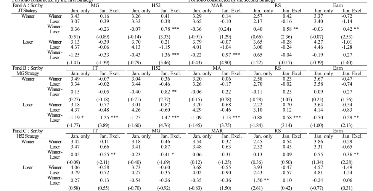
In order to compare the relative profitability of those six momentum strategies, we replicate the pairwise comparisons from George and Hwang (2004). For example, to compare the relative profitability of the JT and the H52 momentum strategy, we first sort all stocks into winner and loser portfolios based on the JT momentum strategy indicators; then all stocks in winner and loser portfolios are once again sorted into winner and loser portfolios based on the 52-week high indicator. If the JT momentum strategy can fully explain profitability of the momentum strategy, the ensuing H52 momentum strategy should not be able to generate any significantly positive return. In other words, the JT momentum strategy outperforms the H52

  9

momentum strategy in this case. Comparison of other pairs of momentum strategies follows the same procedure.

3.4 Simultaneous Comparison

To have a further comprehensive comparison of all six momentum strategies, we adopt the regression framework proposed by George and Hwang (2004). As described in the following regression model, we control the size and value-growth factors, and measure the relative profitability of the six momentum strategies with their winner- and loser- dummy variables included in the model.

0 1 , 1 2 , 1 3 4 , 5 , 6 , 7 , 8 , 9 , 10 , 11 , 12 , 13 , 14 , 15 52 52 it kt kt i t kt i t kt i kt i t k kt i t k kt i t k kt i t k kt i t k kt i t k kt i t k kt i t k kt i t k kt i t k kt i t k k R b b R b Size b BM b JTW b JTL b MGW b MGL b H W b H L b MARW b MARL b RSW b RSL b EarnW b                              _tEarnL_{i t k,} e_it, (8)

where t-k is the portfolio construction period, and k=2,…,7 when the portfolio holding period

is six months;Size_i,t1is the market value of stock i at t-1 month;BM is the book to market _i

ratio of stock i. All the other explanatory variables are dummy variables. For example, JTW=1

indicate that stock i belongs to the winner portfolio of the JT momentum strategy; while JTL=1 indicate that stock i belongs to the loser portfolio of the JT momentum strategy. The

other dummy variables follow similar definitions. For the regression coefficients, b _0kt

represents average return free of size-, value-growth factors, and all momentum effects, while

kt kt b

b₄ ~ ₁₅ represent the winner- and loser- portfolio effects at time t. Since our portfolios are

constructed with overlapping holding periods, return at month t is consist of portfolios

constructed in six different period. Therefore, we follow George and Hwang (2004) in calculating the mean value of each coefficient as

7 7 7

4kt 1_{6 k 2} 4kt 5kt 1_{6 k 2} 5kt .... 15kt 1_{6 k 2} 15kt

  10

6kt 7kt

b b

、 、b_8kt b_9kt、b_10kt b_11kt、b_12kt b_13ktandb_14kt b_15kt to obtain average excess returns of the JT, the MG, the H52, the MAR, the RS and the Earn momentum strategy at month t.

In addition, we also risk-adjust returns with the Fama-French three-factor model, and explore whether the risk-adjusted profitability of momentum strategy exhibits any significant change.

3.5 Robustness Tests

Novy-Marx (2012) demonstrates with American data that momentum effect constructed with returns from the past 7~12 months outperforms those constructed with returns from the past 1~6 months. Therefore, we also include winner- and loser- dummy variables constructed with returns from the past 7~12 months in the regression model of George and Hwang (2004) as follows, 0 1 , 1 2 , 1 3 4 , 5 , 6 , 7 , 8 , 9 , 10 , 11 , 12 , 13 , 1 16 16 712 712 16 16 712 712 52 52 it kt kt i t kt i t kt i kt i t k kt i t k kt i t k kt i t k kt i t k kt i t k kt i t k kt i t k kt i t k kt i t k R b b R b Size b BM b JT W b JT L b JT W b JT L b MG W b MG L b MG W b MG L b H W b H L b                            _{4 , 15 , 16 ,} 17 , 18 , 19 , 20 , 21 , 16 16 712 712 , kt i t k kt i t k kt i t k kt i t k kt i t k kt i t k kt i t k kt i t k it MARW b MARL b RS W b RS L b RS W b RS L b EarnW b EarnL e                 (9)

where JT16W (JT16L), MG16W (MG16L), RS16W (RS16L) are winner- (loser-) dummy variables constructed with returns from the past 1~6 months, while JT712W (JT712L),

MG712W (MG712L), RS712W (RS712L) are winner- (loser-) dummy variables constructed with returns from the past 7~12 months.b_4kt ~b_21kt represent the winner- and loser- portfolio

effects at time t. Letb_4kt  1₆







、b_16kt b_17kt、 b_18kt b_19ktand b_20kt b_21kt to obtain average excess returns of JT16, JT712,

  11

Furthermore, since Cooper and Guterrez (2004) argue the market state as the main reason that contributes to the profitability momentum strategies, and the momentum effect occurs mainly in the bull market. In the paper, we also follow Cooper and Guterrez (2004) in defining a bull (bear) market when the past 36 months market return is non-negative

(negative). We then compare relative profitability of those various momentum strategies in the bull and the bear market states within the regression framework of George and Hwang (2004).

4

Empirical Results

3.1 Profitability of Momentum Strategies

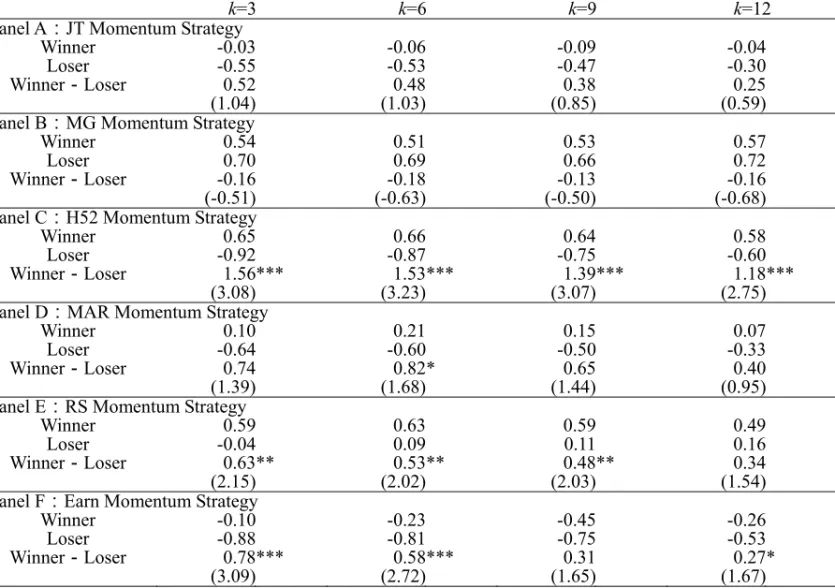
We first discuss whether various momentum strategies generate momentum effect in Taiwan’s stock market. Table 1 presents and compares profitability of the price (JT) momentum strategy, the industry (MG) momentum strategy, the 52-week high (H52) momentum strategy, the moving average (MAR) momentum strategy, the Residual (RS) momentum strategy, and the Earnings (Earn) momentum strategy for holding periods of 3, 6, 9, and 12months, respectively. Panel A and Panel B in Table 1 show no momentum effect for the JT and the MG momentum strategies for all holding periods; Panel C shows significantly positive momentum effect for the H52 momentum strategy, with returns of 1.56%, 1.53%, 1.39% and 1.18%, respectively; Panel D shows that the MAR momentum strategy only exhibits a significantly positive return of 0.82% for a holding period of 6 months; Panel E shows positive returns of 0.63% (3 months), 0.53% (6 months) and 0.48% (9 months) for the RS momentum strategy; Panel F shows significantly positive returns of 0.78% (3 months) and 0.58% (6 months) for the Earn momentum strategy.

To examine whether the profitability of momentum strategy in Taiwan’s stock market is affected by the January effect, we split the sample into January and non-January observations,

  12

re-examine profitability of each momentum strategy and present the results in Table 2. From the non-January columns in Panel A to Panel E, returns to all winner and loser portfolios are positive and outperform those presented in Table 1. This shows that the January effect does exist in Taiwan’s security market. However, returns to almost all momentum strategies are negative for January-only months, which are consistent with the findings in George and Hwang (2004). For non-January months in Table 2, average monthly returns of loser

portfolios of the JT, MG, RS, H52 and MAR momentum strategies become smaller compared to those presented in Table 1, which result in better momentum strategy profit. In addition, the H52 momentum strategy clearly outperforms other momentum strategies for all holding periods. To summarize empirical results in Table 1 and Table 2, we find that all but the JT and the MG momentum strategies show significantly positive momentum effect in Taiwan’s security market. Among all, the H52 momentum strategy exhibits the best momentum effect.

--- Insert Table 1 and Table 2 here

---

4.2 Pairwise Comparison

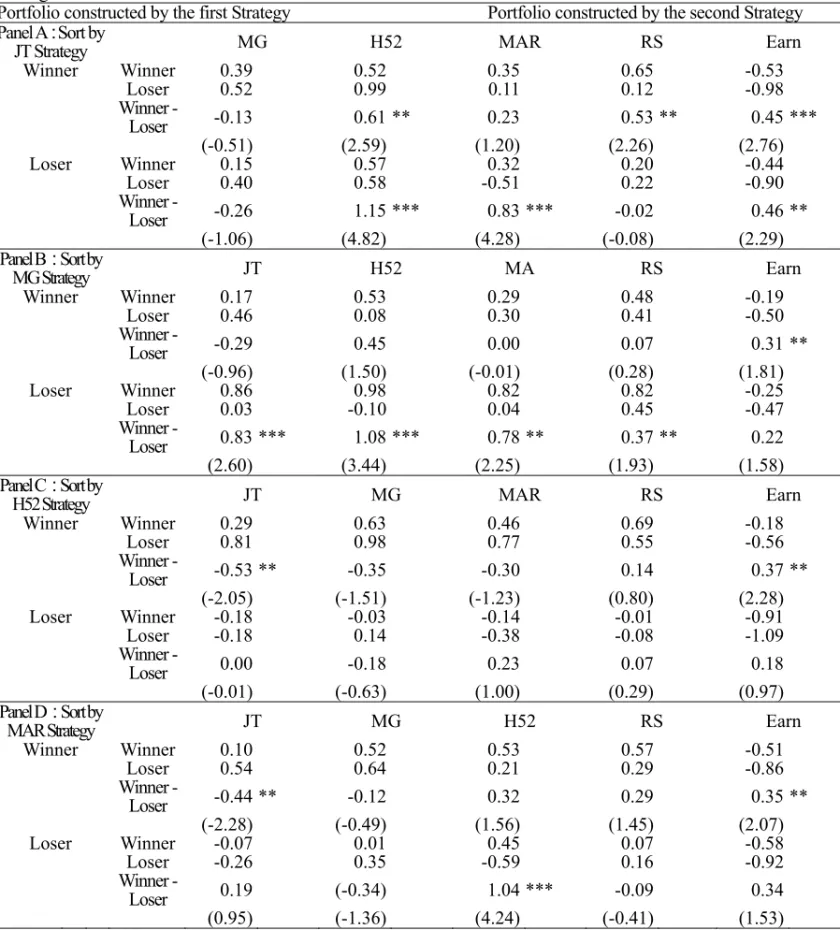
We further compare profitability of momentum strategies with pairwise comparison, and present the results in Table 3 and Table 4. In Panel A of Table 3, a winner (loser) portfolio is first formed with the top (bottom) 30% of stocks sorted by the JT momentum indicator, stocks in the winner and the loser portfolios are further sorted by one of the other five momentum strategy indicators into winner and loser portfolios. The results show that, in the JT winner portfolio (JT loser portfolio), winner-loser portfolio formed by H52, RS and Earn (H52, MAR and Earn) momentum strategies enjoy significant positive monthly returns of 0.61%, 0.53% and 0.45% (1.15%, 0.83% and 0.46%), respectively. Such results demonstrate additional

  13

explanatory power of those other momentum strategies on the returns of portfolios formed by the JT momentum strategy.

In Panel B, a winner (loser) portfolio is first formed with top (bottom) 30% of stocks sorted by the MG momentum strategy, stocks in the winner and the loser portfolios are further sorted by one of the other five momentum strategy indicators into winner and loser portfolios. We find that, in the MG winner portfolio (MG loser portfolio), winner-loser portfolio formed by Earn (JT, H52, MAR and RS) momentum strategies enjoy significant positive monthly returns of 0.31% (0.83%, 1.08%, 0.78% and 0.37%), respectively. Such results demonstrate additional explanatory power of those other momentum strategies on the returns of portfolios formed by the MG momentum strategy.

In Panel C, a winner (loser) portfolio is first formed with top (bottom) 30% of stocks sorted by the H52 momentum strategy, stocks in the winner and the loser portfolios are further sorted by one of the other five momentum strategy indicators into winner and loser portfolios. We find that, only in the H52 winner portfolio, winner-loser portfolio formed by Earn momentum strategies enjoys significant positive monthly returns of 0.37%. Such results demonstrate additional explanatory power of the Earn momentum strategy on the returns of portfolios formed by the H52 momentum strategy.

In Panel D, a winner (loser) portfolio is first formed with top (bottom) 30% of stocks sorted by the MAR momentum strategy, stocks in the winner and the loser portfolios are further sorted by one of the other five momentum strategy indicators into winner and loser portfolios. We find that, in the MAR winner portfolio (MAR loser portfolio), winner-loser portfolio formed by Earn (H52) momentum strategies enjoy significant positive monthly returns of 0.35% (1.04%). Such results demonstrate additional explanatory power of Earn and

  14

H52 momentum strategies on the returns of portfolios formed by the MAR momentum strategy.

In Panel E, a winner (loser) portfolio is first formed with top (bottom) 30% of stocks sorted by the RS momentum strategy, stocks in the winner and the loser portfolios are further sorted by one of the other five momentum strategy indicators into winner and loser portfolios. We find that, in the RS winner portfolio (RS loser portfolio), winner-loser portfolio formed by Earn (H52) momentum strategies enjoy significant positive monthly returns of 0.35% (1.04%). Such results demonstrate additional explanatory power of Earn and H52 momentum strategies on the returns of portfolios formed by the RS momentum strategy.

In Panel F, a winner (loser) portfolio is first formed with top (bottom) 30% of stocks sorted by the Earn momentum strategy, stocks in the winner and the loser portfolios are further sorted by one of the other five momentum strategy indicators into winner and loser portfolios. We find that, only in the Earn loser portfolio, winner-loser portfolio formed by H52 momentum strategies enjoys significant positive monthly returns of 0.72%. Such results demonstrate additional explanatory power of the H52 momentum strategy on the returns of portfolios formed by the Earn momentum strategy.

Summing up the above empirical results, we can find that the H52 and the Earn momentum strategy both offer additional explanatory power to returns of portfolios formed by other momentum strategies. In contrast, few other momentum strategies can offer additional explanatory power to returns of portfolios formed by the H52 and the Earn momentum strategy. Even when the January effect is taken into account, the pairwise comparison results presented in Table 4 show little changes. Such empirical results seem to imply that the H52 and the Earn momentum strategies obviously outperform the other four

  15

momentum strategies.

--- Insert Table 3 ad Table 4 here.

---

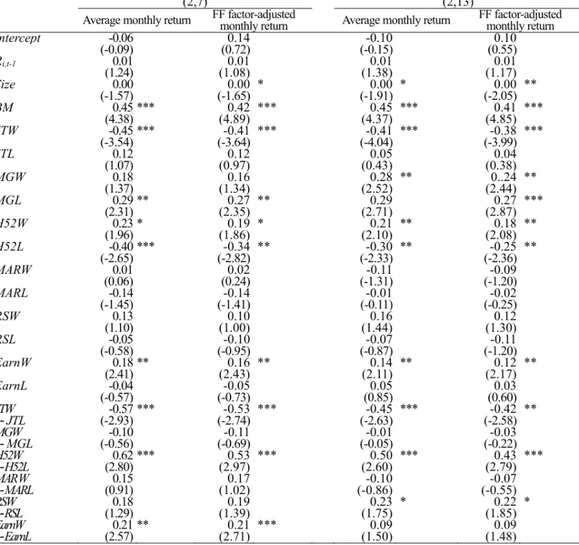
4.3 Simultaneous Comparison of All Momentum Strategies

To further compare the relative profitability of all six momentum strategies, we perform the regression in Equation (8), and present the results in Table 5. Among them, the H52 momentum strategy generates significantly positive returns for a holding period of both 6 and 12 months, which are 0.62% and 0.50%, respectively. Furthermore, even with returns adjusted by the Fama-French three-factor model, the H52 momentum strategy still generates

significantly positive returns for a holding period of both 6 and 12 months, which are 0.53% and 0.43%, respectively. With a holding period of 12 months, the RS momentum strategy enjoys a significantly positive return of 0.23%, and a risk-adjusted return of 0.22%. With a holding period of 6 months, the Earn momentum strategy enjoys a significantly positive return of 0.21%, and a risk-adjusted return of 0.21%.

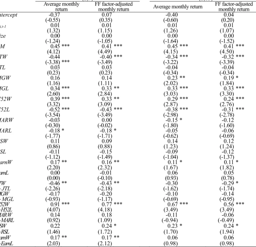
Table 6 presents results of the regression in Equation (8) after excluding observations in January months. Again, the H52 momentum strategy generates significantly positive returns for a holding period of both 6 and 12 months, which are 0.91% and 0.67%, respectively. Even with returns adjusted by the Fama-French three-factor model, the H52 momentum strategy still generates significantly positive returns for a holding period of both 6 and 12 months, which are 0.77% and 0.56%, respectively. With a holding period of 12 months, the RS momentum strategy enjoys a significantly positive return of 0.23%, and risk-adjusted return of 0.24%. With a holding period of 6 months, the Earn momentum strategy enjoys a

  16

significantly positive return of 0.17%, and risk-adjusted return of 0.17%.

The above results show that, by simultaneously comparing those six momentum strategies, the H52, the RS and the Earn momentum strategy can each generate positive momentum effect. However, the momentum effect of the H52 momentum strategy clearly outperforms the other two strategies (RS and Earn) in both the six- and the twelve-months holding periods.

--- Insert Table 5 and Table 6 here

---

4.4 Different Lengths of Portfolio Formation Period

Novy-Marx (2012) demonstrates with American data that momentum effect constructed with returns from the past 7~12 months outperforms those constructed with returns from the past 1~6 months. Based on average returns for the past 1~6 months and 7~12 months, we formed the price-, the industry-, and the residual-momentum strategies, which are denoted as JT16, JT712, MG16, MG712, RS16 and RS712. Table 7 presents profitability of these momentum strategies for holding periods of 3, 6, 9 and 12 months.

Panel A indicates that the JT16 momentum strategy can generate significantly positive returns of 0.72% and 0.70% for holding periods of 6 and 9 months. Panel E indicates that the RS16 momentum strategy can generate significantly positive returns of 0.55% and 0.46% for holding periods of 9 and 12 months. Panel F indicates that the RS712 momentum strategy can generate significantly positive returns of 0.94%, 0.87%, 0.64% and 0.38% for holding periods of 3, 6, 9 and 12 months. To sum up, JT16, RS16 and RS712 momentum strategies all

generate moment effect, with RS712 momentum strategy outperforming the other two momentum strategies.

  17

(2004) by decomposing JT, MG and RS momentum strategies into JT16, JT712, MG16, MG712, RS16 and RS712 as in Equation (9) and present the results in Table 8. The H52 momentum strategy generates significantly positive return for a holding period of 6 (12) months, which is 0.34% (0.27%). The RS712 momentum strategy generates significantly positive return for a holding period of 6 (12) months, which is 0.23% (0.18%). Furthermore, even with returns adjusted by the Fama-French three-factor model, the RS712 momentum strategy still generates a significantly positive return of 0.22% (0.17%) for a holding period of 6 (12) months. The Earn momentum strategy generates significantly positive return for a holding period of 6 (12) months, which is 0.29% (0.10%). Furthermore, even with returns adjusted by the Fama-French three-factor model, the Earn momentum strategy still generates a significantly positive return of 0.29% for a holding period of 6 months.

Table 9 is similar to Table 8 except that observations in January months are excluded. The H52 momentum strategy generates significantly positive return for a holding period of 6 (12) months, which is 0.50% (0.48%). With returns adjusted by the Fama-French three-factor model, the H52 momentum strategy still generates a significantly positive return of 0.38% (0.36%) for a holding period of 6 (12) months. The RS712 momentum strategy generates significantly positive return for a holding period of 6 (12) months, which is 0.28% (0.21%). With returns adjusted by the Fama-French three-factor model, the RS712 momentum strategy still generates a significantly positive return of 0.27% (0.21%) for a holding period of 6 (12) months. The Earn momentum strategy generates significantly positive return (0.24% for both the raw and the risk-adjusted) for a holding period of 6 months.

Combining the empirical results in Table 8 and Table 10, the H52 momentum strategy for holding periods of both 6 and 12 months still outperform other momentum strategies.

  18

--- Insert Table 7, Table 8, and Table 9 here.

---

4.5 Different Market States

Table 10 presents results that simultaneously compare profitability of various momentum strategies in the bull and the bear market states within the regression framework of George and Hwang (2004). Panel A show that, in the bull market state, the H52 momentum strategy can generate a significantly positive average return of 0.61% (0.59%) for a holding period of 6 (12) months. In addition, even with returns adjusted by the Fama-French three-factor model, the H52 momentum strategy can still generate a significantly positive return of 0.34% for a holding period of 12 months. The RS momentum strategy can generate a significantly positive average return of 0.28% (0.26%) for a holding period of 6 (12) months. In addition, even with returns adjusted by the Fama-French three-factor model, the RS momentum strategy can still generate a significantly positive return of 0.34% (0.27%) for a holding period of 6(12) months. The Earn momentum strategy can generate a significantly positive average return of 0.19% for a holding period of 6 months. In addition, even with returns adjusted by the Fama-French three-factor model, the Earn momentum strategy can still generate a significantly positive return of 0.22% for a holding period of 6 months. Panel B in Table 10 shows that, in the bear market state, none of the momentum strategies can generate significantly positive average return.

Table 11 is similar to Table 10 except that observations in January months are excluded. Panel A show that, in the bull market state, the H52 momentum strategy can generate a significantly positive average return of 1.06% (0.85%) for a holding period of 6 (12) months.

  19

In addition, even with returns adjusted by the Fama-French three-factor model, the H52 momentum strategy can still generate a significantly positive return of 0.66% (0.50%) for a holding period of 6 (12) months. The RS momentum strategy can generate a significantly positive average return of 0.35% (0.28%) for a holding period of 6 (12) months. In addition, even with returns adjusted by the Fama-French three-factor model, the RS momentum strategy can still generate a significantly positive return of 0.46% (0.31%) for a holding period of 6(12) months. The Earn momentum strategy can generate a significantly positive average return of 0.19% for a holding period of 6 months, with returns adjusted by the Fama-French three-factor model. Panel B in Table 11 shows that, in the bear market state, none of the momentum strategies can generate significantly positive average return.

Combining the empirical results in Table 10 and Table 11, we fins that. In the bull market state, the H52 and the RS momentum strategies for holding periods of 6 and 12 months can both produce momentum effect, while the Earn momentum strategy can only produce momentum effect with a holding periods of 6 months. In contrast, in the bear market state, none of the momentum strategies can generate significantly positive average return. These are consistent with the findings in Cooper and Guterrez (2004).

--- Insert Table 10 and Table 11 here.

---

5

Conclusions

This paper examines relative profitability of six popular momentum strategies in Taiwan’s stock market, namely the price-, the industry-, the 52-week high-, the moving

  20

average ratio-, the residual-, and the earnings-momentum strategies. Our empirical results show that the 52-week high-, the residual-, and the earnings-momentum strategies can all generate significantly positive returns, with the return of the 52-week high being the highest. After excluding observations in January months, returns to loser portfolios of most

momentum strategies become smaller, which result in even better returns of momentum portfolios. This indicate a clear impact of the January effect on the performance of momentum strategies.

With pairwise comparison, the 52-week high- and the earnings-momentum strategies both provide additional explanatory power to returns conditional on the other four momentum strategies. In contrast, the other four momentum strategies do not offer additional explanatory power to returns conditional on the 52-week high- or the earnings-momentum strategies. Furthermore, following George and Hwang’s (2004) regression model, we conduct a

simultaneous comparison of the six momentum strategies, and find that the profitability of the 52-week high momentum strategy is significantly better than other strategies. Overall, the 52-week high-momentum strategy stands out as the most profitable momentum indicator in Taiwan’s stock market.

For robustness tests, we find that momentum effect constructed with returns from the past 7~12 months are qualitatively similar to those constructed with returns from the past 1~6 months, with the profitability of the 52-week high-momentum strategy being the highest. Furthermore, with different market states, we find that the 52-week high-, the residual-, and the earnings-momentum strategies can all produce momentum effect in the bull market state, while none of the momentum strategies can generate significantly positive average return in the bear market state. These findings are consistent with the findings in Cooper and Guterrez

  21

(2004).

Overall, the 52-week high-momentum strategy stands out as the most profitable momentum indicator in Taiwan’s stock market.

  22

References

1. Blitz, David, Joop Huij and Martin Martens, 2011. Residual Momentum, Journal of

Empirical Finance, 18(3), 506-521.

2. Chan, Louis K. C., Narasimhan Jegadeesh and Josef Lakonishok, 1996. Momentum Strategies, Journal of Finance, 51(5), 1681-1713.

3. Cooper, Michael J. and Roberto C. Gutierrez JR., 2004. Market States and Momentum,

Journal of Finance, 59(3), 1345-1365.

4. Fama, Eugene F. and Kenneth R. French, 1992. The Cross-Section of Expected Stock Returns, Journal of Finance, 47(2), 427-465.

5. Fama, Eugene F. and Kenneth R. French, 1993. Common Risk Factors in the Returns on Stocks and Bonds, Journal of Financial Economics, 33(1), 3-56.

6. George, Thomas J. and Chuan-Yang Hwang, 2004. The 52-Week High and Momentum Investing, Journal of Finance, 59(5), 2145-2176.

7. Jegadeesh, Narasimhan and Sheridan Titman, 1993. Returns to Buying Winners and Selling Losers: Implications for Stock Market Efficiency, Journal of Finance, 48(1), 65-91.

8. Lo, Andrew W. and A. Craig Mackinlay, 1990. Data-Snooping Biases in Tests of Financial Asset Pricing Models, Review of Financial Studies, 3(3), 431-467.

9. Novy-Marx, Robert, 2012. Is Momentum Really Momentum? Journal of Financial

Economics, 103(3), 429-453.

10. Moskowitz, Tobias J. and Mark Grinblatt, 1999. Do Industries Explain Momentum?

Journal of Finance, 54(4), 1249-1290.

  23

45(2), 415-447.

12. Schwert, G. William, 2002. Anomalies and Market Efficiency, in Handbook of the

Economics of Finance, edited by G.M. Constantinides, Harris, M. and R. Stulz, pp.