國 立 交 通 大 學
電機與控制工程學系
碩 士 論 文
探討動態刺激對不同的認知狀態下
腦神經活化的影響
Effects of Kinesthetic Stimulation on Neural
Activities under Different Cognitive States
研 究 生: 陳 明 達
指導教授: 林 進 燈 教授
探討動態刺激對不同的認知狀態下
腦神經活化的影響
Effects of Kinesthetic Stimulation on Neural
Activities under Different Cognitive States
研 究 生:陳明達 Student:
Min-Ta Chen
指導教授:林進燈 博士
Advisor:Dr. Chin-Teng Lin
國立交通大學
電機與控制工程學系
碩士論文
A Thesis
Submitted to Department of Electrical and Control Engineering
College of Engineering and Computer Science
National Chiao Tung University
in Partial Fulfillment of the Requirements
for the Degree of Master
in
Electrical and Control Engineering
June 2007
Hsinchu, Taiwan, Republic of China
授 權 書
(碩士論文)
本授權書所授權之論文為本人在 國立交通 大學 電機 學院 電機與控制工程 系所 資訊智慧 組 九十五 學年度第 二 學期取得 碩 士學位之論文。
論文名稱:探討動態刺激對不同的認知狀態下腦神經活化的影響
Effects of Kinesthetic Stimulation on Neural Activities under Different Cognitive States
1. 5同意 不同意 本人具有著作財產權之論文全文資料,授予行政院國家科學委員會科學技術資料中心、 國家圖書館及本人畢業學校圖書館,得不限地域、時間與次數以微縮、光碟或數位元化 等各種方式重製後散佈發行或上載網路。本論文為本人向經濟部智慧財產局申請專利的 附件之一,請將全文資料延後兩年後再公開。 (請註明文號: ) 2. 5同意 不同意 本人具有著作財產權之論文全文資料,授予教育部指定送繳之圖書館及本人畢業學 校圖書館,為學術研究之目的以各種方法重製,或為上述目的再授權他人以各種方 法重製,不限地域與時間,惟每人以一份為限。 上述授權內容均無須訂立讓與及授權契約書。依本授權之發行權為非專屬性發行權利。 依本授權所為之收錄、重製、發行及學術研發利用均為無償。上述同意與不同意之欄位 若未鉤選,本人同意視同授權。 指導教授姓名: 林 進 燈 教授 研 究 生簽名: 學號: 9412603 (親筆正楷) (務必填寫) 日 期: 民國 九十六 年 八 月 日 1. 本授權書請以黑筆撰寫並影印裝訂於書名頁之次頁。 2. 授權第一項者,所繳的論文本將由註冊組彙總寄交國科會科學技術資料中心。 3. 本授權書已於民國 85 年 4 月 10 日送請內政部著作權委員會(現為經濟部智慧財產 局)修正定稿。 4. 本案依據教育部國家圖書館 85.4.19 台(85)圖編字第 712 號函辦理。
探討動態刺激對不同的認知狀態下
腦神經活化的影響
學生:陳明達
指導教授:林進燈 博士
國立交通大學電機與控制工程研究所
Chinese Abstract中文摘要
在長時間或單調的駕車環境裡,駕駛很容易減低他們的警覺心或注意力。昏睡的駕 駛沒辦法專心地開車,會導致一些錯誤的車輛操縱。他們處理訊息的速度與記憶的能力 都變差,而開車技巧隨著警覺心的降低開始變糟。之前的研究大多是在靜態的開車環境 裡,利用行為上的狀態或生理訊息去預測駕駛的昏睡程度。然而有一些研究發現動態的 刺激會影響腦電波(electroencephalogram, EEG)α頻帶(8~12 Hz)能量的變化,並且當 成警覺心的指標。在真實的駕駛裡,動態刺激對利用神經活動偵測昏睡程度準確性影響 的程度仍是未知。因此我們研究的目的在於有系統的描述動態刺激對不同認知程度的大 腦活動影響,特別是在昏睡的部份。 我們利用虛擬環繞場景結合六軸動態平台,獨立成份分析(Independent Component Analysis, ICA)和時頻分析研究從清醒到昏睡時的腦電波活動,並比較平台動與不動的 差異。本實驗結果顯示,當受測者昏睡程度增加,使其駕車的能力下降,發現此時大腦 枕葉區(occipital)在偏移事件發生前之腦波的α頻帶能量會增加。相似昏睡程度也使 偏移事件發生後之腦波的α頻帶能量下降的時間點延後,並增加持續下降的時間。在相 同的行為反應下去觀察平台動時腦電波從清醒到昏睡的變化比平台不動時更明顯。本研 究的結果第一次證明了動態刺激對虛擬駕車環境的重要性,更進一步指出腦電波的變化 比行為狀態更能靈敏地反應出駕駛的昏睡狀態。 關鍵字︰動態刺激、昏睡程度、腦電波、獨立成份分析、時頻分析、功率頻譜、暫態α 頻帶能量下降Effects of Kinesthetic Stimulation on Neural
Activities under Different Cognitive States
Student: Min-Ta Chen
Advisor: Dr. Chin-Teng Lin
Department of Electrical and Control Engineering National Chiao Tung University
English Abstract
Abstract
It has been found that drivers easily to reduce their vigilance or attention during the prolonged or monotonous driving. The drowsy driver can’t focus on their driving task and tend to commit on manipulating errors. Their information processing speed and working memory capacities are decreased and drastic changes on their task performance occur along with the reduction of the vigilance. Most previous studies that tried to figure out the useful features from behavioral performances or physiological signals for predicting driver’s drowsiness level were done in a static driving environment. However, some studies already showed that the kinesthetic stimulus had influences on fluctuations of brain dynamics especially near the alpha band power, which already used as an index of the vigilance. To what extent the kinesthetic stimulation would affect the accuracy on the predicting drowsiness level from neural activities in real driving is still unclear. Therefore, the aim of this study is to systemically characterized effects of kinesthetic stimulation on the brain activities under different cognitive state, particularly under the drowsiness condition.
We used the 3 dimensional surrounded virtual reality scene combined with the six degree motion platform, the independent component analysis (ICA) and time-spectral analysis to explore the fluctuations in spectral dynamics of maximally independent EEG activities from
alter to drowsy with or without the enabling of the motion platform. Results showed that subjects’ drowsiness level was increased with the deteriorated of the driving performance which reflected on the tonic increases of the power spectral baselines near the alpha band in the occipital components. The similar drowsy effects also revealed on the changes of the phasic alpha suppressions including the delaying its onset and increases its mean prevalence. With the same behavioral performances, changes on EEG dynamics from alert to drowsiness were further enhanced when the motion platform was enabled. Results of this study first demonstrated the importance of the kinesthetic stimulation in the simulated driving studies. Furthermore, this study also first revealed that the EEG dynamics is more sensitive than the behavioral performance for correctly detecting driver’s drowsiness level.
Keyword: Kinesthetic Stimulus, Drowsiness level, EEG, ICA, time-frequency analysis, power spectral baselines, phasic alpha suppression
誌 謝
Acknowledgement 本論文的完成,首先要感謝我的指導教授 林進燈博士在過去兩年研究期間,提供 豐富的研究資源和實驗環境,並從旁指導協助,使得本文得以順利完成。 其次,我要感謝我的父母對我的照顧與栽培,教導我做人品德為最,強調人格健全 之發展與學習生活之態度,由於他們辛勞的付出和細心的照顧,才有今天的我。 特別感謝 曲在雯博士對我研究的指導還有幫忙論文的修改,使我學到許多東西。 還有 梁勝富教授、蕭富仁教授、林文杰教授給予我在各方面的指導,無論是研究上疑 難的解答、研究方法、寫作方式、經驗分享等惠我良多。 感謝美國加州聖地牙哥大學的 鐘子平教授、 段正仁教授及 黃瑞松學長,給予我 研究上最大的協助,從實驗設計、實驗分析、實驗結果討論到論文撰寫,給我最專業的 意見跟看法。 另外,我要感謝腦科學研究實驗室的全體成員,沒有他們也就沒有我個人的成就。 另外要感林弘章、鄭仲良、趙志峰同學,在過去兩年研究生活中同甘共苦,相互扶持。 此外,我也要感謝陳玉潔學姊、柯立偉學長與黃騰毅學長在研究上的幫助,還有感謝柏 銓、玠遙、奎銘、德正、孟修、青甫以及尚文學弟,在過去這一年中的相伴。同樣地也 感謝實驗室助理在許多事務上的幫忙。 最後,還要感謝許多比我自己更關心我,比我更肯定我的人們,尤其是曾陪我四年 的你,替我分擔許多研究上的壓力與挫折,也讓我在研究所的生活當中,增添更多色彩。 謹以本文獻給我親愛的家人與親友們,以及關心我的師長,願你們共享這份榮耀與 喜悅。Contents
1. Introduction ... 1
1.1. Current researches of drowsiness ... 1
1.2. Kinesthetic perception during driving ... 2
1.3. Virtual reality dynamic simulator ... 3
1.4. Aims of this thesis ... 4
2. Materials and Methods ... 5
2.1. Subjects... 5
2.2. Experimental setup ... 5
2.2.1 Dynamic driving environment... 6
2.2.2 VR scene... 6
2.2.3 Stewart motion platform... 7
2.3. EEG recording ... 8
2.4. Experimental paradigm... 9
2.5. Data analyses ... 11
2.5.1 Analysis of driving performance ... 11
2.5.2 EEG ... 13
2.5.2.1. Independent Component Analysis (ICA) ... 16
2.5.2.2. Time frequency analysis and Event Related Spectral Perturbations (ERSPs) ... 20
2.5.3 Clustering ... 21
2.5.4 Statistics... 23
3. Results... 24
3.1 Behavioral performance ... 25
3.2 Independent Component (IC) clustering ... 29
3.3 Tonic brain dynamics at a large time scale ... 31
3.3.1 Within subjects phenomena ... 31
3.3.2 Cross subject consistency ... 36
3.4 Event-Related Spectral Perturbations (ERSPs) ... 39
3.4.1 The occipital component ... 39
3.4.2 The motor component... 45
3.4.3 The central component ... 50
3.5 The onset of the alpha suppression... 51
4. Discussion ... 55
4.1. Effects of drowsiness on long-term tonic variations ... 55
4.2. Effects of drowsiness on phasic responses ... 56
4.3. Effects of kinesthetic stimulation on the drowsiness level... 57 4.4. The variation of EEG dynamics is potential as a good index for detecting driver’s
drowsiness in real driving... 58
5. Conclusion ... 59 Reference ... 60
Figures
Figure 2-1: The experimental environment ... 5
Figure 2-2: The dynamic VR driving environment ... 6
Figure 2-3: The overview of surrounded VR scene... 7
Figure 2-4: The Stewart platform ...7
Figure 2-5: The International 10-20 system of electrode placement... 8
Figure 2-6: The photographic picture of NuAmps EEG amplifier and the electrode cap... 9
Figure 2-7: The picture of the four-lane highway scene... 10
Figure 2-8: Illustration of the deviation event ... 10
Figure 2-9: The illustration of single deviations ... 12
Figure 2-10: (A) Driving trajectory of a session. (B) The driving error of a session... 12
Figure 2-11: (A) Sorted trials by driving error. (B) Sorted trials by reaction time... 12
Figure 2-12: The cumulative plots of response time from one subject ... 13
Figure 2-13: The flow chart for EEG analysis ... 14
Figure 2-14: Criteria for artifact rejection ... 15
Figure 2-15: Scalp topography of ICA decomposition... 19
Figure 2-16: The flow chart of ERSP analysis ... 21
Figure 2-17: Component selection preceding clustering... 22
Figure 2-18: The scalp maps for the occipital independent component (IC) cluster ... 22
Figure 3-1: The cumulative percentage plots of the response time from ten subjects ... 25
Figure 3-2: The same data as in the Fig. 3-1 but displayed as the response time histograms .. 26
Figure 3-3: The cumulative percentage plots of the response time and their corresponded response histograms of the subject 5 ... 27
Figure 3-4: The response time histogram of fast and slow groups of 4 subjects ... 27
Figure 3-5: The response time histogram of fast and slow groups of 6 subjects ... 28
Figure 3-6; The scalp maps for the occipital independent component (IC) cluster ... 29
Figure 3-7: The scalp maps for the left Mu rhythm IC cluster... 30
Figure 3-8: The scalp maps for the right Mu rhythm IC cluster... 30
Figure 3-9: The scalp maps for the Central IC cluster ... 30
Figure 3-10: showed the grand mean power spectral baselines and the averaged scalp maps of the four IC clusters ... 31
Figure 3-11: showed the grand mean power spectral baselines and the averaged scalp maps of the four IC clusters ... 32
Figure 3-12: The averaged baseline power spectra of 2 subjects ... 32
Figure 3-13: The averaged baseline power spectra of 4 subjects ... 33
Figure 3-14: The averaged baseline power spectra of 4 subjects ... 34
Figure 3-15: The averaged baseline alpha power of ten subjects... 35 Figure 3-16: The grand mean (±SEM) baseline power spectra of two groups of epochs for
four ICs ... 36 Figure 3-17: The effects of kinesthetic stimulus and cognitive status on the averaged baseline
alpha power from ten subjects. ... 37 Figure 3-18: The kinesthetic stimulus significantly increased the difference of the baseline
alpha power between the fast and slow response groups ... 37 Figure 3-19: The ERSP images of occipital component for fast and slow epochs in motionless
and motion session of subject 5... 39 Figure 3-20: The ERSPs of the occipital component for fast and slow epochs in motionless
and motion sessions of subject 1 and 2... 40 Figure 3-21: The ERSPs of the occipital component for fast and slow epochs in motionless
and motion sessions of subject 3, 4 and 6... 41 Figure 3-22: The ERSPs of the occipital component for fast and slow epochs in motionless
and motion sessions of subject 7, 8 and 9... 42 Figure 3-23: The ERSPs of the occipital component for fast and slow epochs in motionless
and motion sessions of subject 10. ... 43 Figure 3-24: The grand mean of ERSP images of occipital component for fast and slow
epochs in motionless and motion sessions across ten subjects... 43 Figure 3-25: Percentage of the 0-5 sec post-deviation epochs with significant (p<0.01) phasic
power decreases, averaged across ten subject ... 44 Figure 3-26: The ERSP images of right mu component for fast and slow epochs in motionless
and motion session of subject 5... 45 Figure 3-27: The ERSP images of right mu component for fast and slow epochs in motionless
and motion session of subject 1, 3, and 6 ... 46 Figure 3-28: The ERSP images of right mu component for fast and slow epochs in motionless
and motion session of subject 7 and 9 ... 47 Figure 3-29: The grand mean of ERSP images of left and right mu component for fast and
slow epochs in motionless and motion session from ten subjects... 48 Figure 3-30: Percentage of the 0-5 sec post-deviation epochs with significant phasic power
decreases, averaged across ten subjects’ left and right mu components ... 49 Figure 3-31: The ERSP images of central IC for fast and slow epochs in motionless and
motion session of subject 5... 50 Figure 3-32: The grand mean of ERSPs of the central IC for fast and slow epochs in
motionless and motion sessions from ten subjects ... 51 Figure 3-33: Averaged time courses of the alpha band for fast and slow epochs in motionless
and motion sessions across ten subjects ... 52 Figure 3-34: Averaged time courses of the alpha band at the mu components in fast and slow
epochs during motionless and motion sessions across ten subjects ... 53 Figure 3-35: Effects of kinesthetic stimulation and changes of response performance on the
Tables
Table 3-1: Subject list ... 24
Table 3-2: The mean baseline alpha power for ten subjects ... 38
Table 3-3: The averaged baseline alpha power from ten subjects ... 38
Table 3-4: The averaged onset of the alpha suppression in the occipital components ... 54
Table 3-5: The mean onset of the alpha suppression in the right mu components... 54
1. Introduction
Drowsy drivers have been identified as the main leading cause of car accidents. It is estimated that there are 76,000–100,000 car crashes occurring each year in the United States, leading to 1500 deaths and thousands of injuries (Knipling and Wang, 1995; Wang et al., 1996). Drowsy drivers cannot focus on driving and tend to commit on manipulating errors. Their information processing speed and working memory capacities are decreased and drastic changes on their task performance occurs (Wylie et al., 1996; Chang and Mannering, 1999; Kostyniuk et al., 2002; Hendrix, 2002). Through face to face interviews with 593 long-distance drivers, McCartt reported that 47 % of the respondents had ever fallen asleep and 25.4% had fallen asleep during driving of the past year (McCartt et al., 2000). Several factors contribute to the occurrence of symptoms of fatigue and falling asleep in drivers, such as lack of sleep, long driving hours, driving in a monotonous environment, taking sedative drugs or drinking alcohol before driving and driving at midnight, early morning, or mid-afternoon hours. Therefore, accurate and non-intrusive real-time monitoring of driver's drowsiness would be highly desirable, particularly if this measurement could be further used to predict changes in driver's performance capacity.
1.1. Current researches of drowsiness
There are several ways to detect drivers’ drowsiness. For example, it can be directly captured from video images (Summala et al., 1999), the rate and duration of the EOG (electrooculogram, Horne and Reyner, 1996). It can also be estimated from bio-signals such as ECG (electrocardiogram), body pressure, and respiration (Milosevic, 1997; Chung et al., 1999), and the electroencephalogram (Horne and Reyner, 1995; Khardi and Vallet, 1994; Lal and Craig, 2002, Huang et al., 1996; Vuckovic et al., 2002; Roberts et al., 2000; Khalifa et al.,
The abundant information in EEG recording can be related to drowsiness, arousal, sleep, and attention (Santamaria and Chiappa, 1987). Previous studies showed that changes in the EEG theta band and the alpha band reflect cognitive and memory performance (Klimesch, 1999). For example, Makeig and Jung (1996) and Huang et al. (2005) reported that mean activity levels in the (< 4 Hz) delta and (4-6 Hz) theta bands, and at the sleep spindle frequency (14 Hz) as well as the baseline alpha band power were significantly increased from alert to poor/drowsy performance. Several EEG studies related to driving also suggested that alpha-band and theta-band power increased as the alertness level of the driver decreased (Torsvall and Akerstedt, 1987; Eoh et al., 2005; Otmani et al., 2005). Though many studies on the driver’s drowsiness with EEG have been performed, the driving simulation apparatus of experiments in the literatures are mostly constructed only on the monitors. But, the static driving simulation is difficult to approach the realistic driving condition, such as the vibrations that would be experienced when driving an actual vehicle on the road.
1.2. Kinesthetic perception during driving
The driving motion is one of the most experienced kinesthetic perceptions in our life, in other word, the perception we sensed during the vehicle speed or direction change. Whenever the vehicle accelerates, decelerates or curves in a corner, we experience a force pulling our body against the direction of moving. For a driver, the perception to motion includes kinesthetic and visual stimulus. A driver does not sense only the pushing or pulling his/her body by a force, but also the scene change related to vehicle movement. The driving perception includes the co-stimulation of visual cue, vestibular stimulation, muscle reaction and skin pressure. It is indeed a complicated mechanism to understand.
There are numbers of difficulties in investigating the driving perception. First of all, the safety of subject must be guaranteed. Experiments should be held under a safe driving
environment, it is very dangerous to conduct driving experiments on the road. Second, appropriate monitoring and data acquisition are needed to study the influence of kinesthetic stimuli. The stimulation should be simple enough and repeatable to keep experiment under control. Third, objective evaluation should be assessed in the studies.
One of the solutions is to conduct driving experiments using a realistic simulator, which is widely used in driving related researches (Kemeny and Panerai, 2003). For the necessity of motion during driving, literatures showed that the absence of motion information increased reaction times to external movement perturbations (Wierville et al., 1983), and decreased safety margins in the control of lateral acceleration in curve driving (Reymond et al., 2001). In real driving, improper signals from disordered vestibular organs were reported to determine inappropriate steering adjustment (Page and Gresty, 1985). Moreover, the presence of vestibular information in driving simulators shows the importance for it influences the perception of illusory self-tilt and illusory self-motion (Groen et al., 1999). All the above studies emphasized the importance of motion perception during driving with the assessment of driving performance and behavior. Our previous studies also demonstrated that multiple cortical EEG sources responded to driving events differentially in dynamic and static environment. Specifically, the alpha band variations occurred in many components (Mu, parietal and occipital) during driving, especially when the vehicle is moving. It is still unclear to what extent the kinesthetic stimulation would interfere with the fluctuations of driver's global level of drowsiness accompanying changes in driver's performance.
1.3. Virtual reality dynamic simulator
Virtual reality (VR) technology is gradually being recognized as a useful tool for the study and assessment of normal and abnormal brain function, as well as for cognitive rehabilitation. Virtual Environments (VE) are created by powerful computers that generate
realistic animated graphics in three dimensions. Creating carefully controlled, dynamic, 3D stimulus environments combined with physiological and behavioral response recording can be offer more assessment options that are not available by traditional neuropsychological methods.
The VR technique allows subjects to interact directly with a virtual environment rather than monotonic auditory and visual stimuli. It is an excellent strategy for brain research on interactive and realistic tasks due to low cost and avoiding risk of operating on the actual machines. In recent years, some researchers designed the VR senses to provide the appropriate environments for brain activity study (Bayliss and Ballard, 2000; Eoh et al., 2005; Huang T.Y et al., 2005). Integrating the VR scene with dynamic motion platform is excellent for studying the influence of kinesthetic stimulus on cognitive state. Therefore, a VR-based dynamic motion platform combined with EEG measured system is an innovation in brain and cognitive engineering researches.
1.4. Aims of this thesis
Aims of this thesis were (1) to characterize EEG changes with the degradation of the alertness and (2) to assess EEG dynamics in responses to kinesthetic stimulus in different cognitive states. We first constructed a Virtual-Reality interactive driving environment consisting of a highway scene and a six degree-of-freedom (6-DOF) motion platform. Then, we designed a lane-keeping driving experiment to indirectly quantify driver’s drowsiness level (Philip et al., 2003). Therefore, we could easily demonstrate that changes of EEG activities were correlated with driver’s response performance as well as the influences of kinesthetic stimulation on EEG dynamics from alter to drowsiness. Accordingly, this thesis provided strong evidences to show that the dynamic motion platform is required for correctly estimating driver’s cognitive states under driving in the future.
2. Materials and Methods
2.1. Subjects
Ten right-handed healthy adults (9 males, 1 female; age range 22~25 years, mean= 23.5, SD = 0.7) with normal or corrected to normal vision were paid to participate in this experiment. All subjects were free of neurological or psychiatric disorders. In order to let subjects easily fell asleep during the experiment, subjects were asked to have the lunch or dinner at 1hr before the experiment. Subjects practiced the driving task for 5-10 min for reaching the satisfactory performance after the placement if the EEG cap and electrodes. Each subject at least had to complete two 100-minute sessions in two different days.
2.2. Experimental Setup
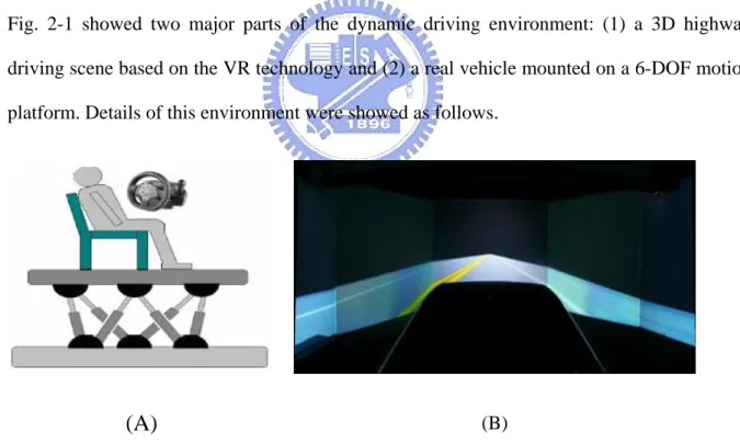
Fig. 2-1 showed two major parts of the dynamic driving environment: (1) a 3D highway driving scene based on the VR technology and (2) a real vehicle mounted on a 6-DOF motion platform. Details of this environment were showed as follows.
(A)
(B)Figure 2-1: The dynamic VR driving environment. (A) Dynamic Driving Simulator. (B) Virtual-Reality Scene.
2.2.1. Dynamic driving environment
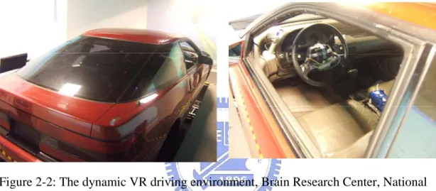
The dynamic driving environment provided a safe, time saving and low cost approach to study human cognition under realistic driving events. Our driving simulator provided not only high-fidelity VR scene, but also kinesthetic inputs and realistic driving environment (as shown in Fig. 2-2). These could make subjects feel that they were driving in a real vehicle on the real road.
Figure 2-2: The dynamic VR driving environment, Brain Research Center, National Chiao Tung University, Taiwan, ROC
2.2.2. VR scene
The VR-based high-fidelity 3D interactive highway scene was developed by using the WorldToolKit (WTK) 3D engine. The 3D view was composed of seven identical PCs running the same VR program and the seven PCs were synchronized by LAN that all scenes were going at exactly same pace. The VR scenes of different viewpoints were projected on corresponding locations.
Literatures showed that the horizontal field of view (FOV) of 120° is needed for correct speed perception (Jamson, 2000). In our VR scenes, the surrounded screens covered 206° frontal FOV and 40° back FOV (Fig. 2-3). Frames projected from 7 projectors were
connected side by side to construct a surrounded VR scene. The size of each screen had diagonal measuring 2.6-3.75 meters. The vehicle was placed at the center of the surrounded screens.
Figure 2-3: The overview of surrounded VR scene. The VR-based four-lane highway scenes are projected into surround screen with seven projectors.
2.2.3. Stewart motion platform
The Stewart motion platform had a lower base platform and an upper payload platform connected by six extensible legs with ball joints at both ends (Fig. 2-4). The platform generated accelerations in vertical, lateral and longitudinal direction of vehicle as well as pitch, roll and yaw angular accelerations.
(A) (B) Figure 2-4: The Stewart platform. (A) The sketch map for the Stewart platform. (B)
2.3. EEG recording
Subjects were with a movement-proof electrode cap with 36 sintered Ag/AgCl electrodes for measuring the electrical activates of the brain and that is the electroencephalogram (EEG). Electrodes were positioned according to the standard international 10-20 system (as shown in Figure 2-5). Active sites were referenced to linked left and right mastoids. EEG signals were recorded and amplified by the Scan NuAmps Express system (Compumedics Ltd., VIC, Australia, Fig. 2-6) with a sampling rate at 500 Hz and 16-bit precision. Data were first filtered with a low-passed filtering with a cut-off frequency at 50Hz for removing the power line noise and other high frequency noise. Then, a high passed filtering with the cut-off frequency at 0.1 Hz was applied to remove the baseline drifts. At the end of each completely session, the location of the electrodes were digitized with the 3D digitizer (POLHEMUS 3 space eastrak).
(A) (B) Figure 2-5: The International 10-20 system of electrode placement. (A) Lateral view. (B)
Top view. (http://faculty.washington.edu/chudler/1020.html) .
Figure 2-6: The photographic picture of NuAmps EEG amplifier and the electrode cap.
2.4. Experimental paradigm
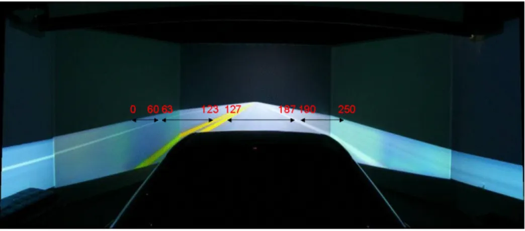
A virtual-reality (VR) based highway-driving environment developed in our previous studies was used to investigate drivers’ cognitive changes in a long-term driving task. The four lanes from left to right were separated by a median strip. The distance between the left and right sides of the road was equally divided into 250 points (digitized into values 0–250 show as Fig. 2-7), where the width of each lane and the car was 60 and 32 units, respectively.
Figure 2-7: The picture of the four-lane highway scene. The distance from the left to the right side of the road was equally divided into 250 points.
The refresh rate (60Hz) of highway scene was set properly to emulate a car driving at a fixed speed of 100 km/hr on the highway. All scenes were moving according to the displacement of the car and the subject’s wheel handling as show in Fig. 2-8.
Figure 2-8: Illustration of the deviation event. (A) Vehicle moving in straight line. (B) Deviation event occurred. (C) Subject’s reaction. (D) Vehicle back to middle lane.
The car was randomly drifted (triggered from the WTK program and the on-set time is recorded) away from the center of the cruising lane to mimic the consequences of a non-ideal road surface. The task required subjects to keep the car on the center of third cruising lane (from left to right counted) during the experiment. The inter-deviation intervals were varied from 5 to 10 sec and the car deviated either left or right with the equal chance. Subjects were instructed to continue to perform the task as best as they could even if they began to feel drowsy. The deviation onset time and the subject’s reaction time were recorded 60 times per second via a synchronous pulse marker train that was recorded in parallel by the EEG acquisition system for the further analysis.
For determining effects of kinesthetic stimulus on the neural activities under different cognitive status in a long term driving tasks, this experiment contained two different conditions: the “motion” and “motionless”. These two conditions were achieved by enabling or disabling the motion platform action.
2.5. Data Analyses
2.5.1. Analysis of driving performance
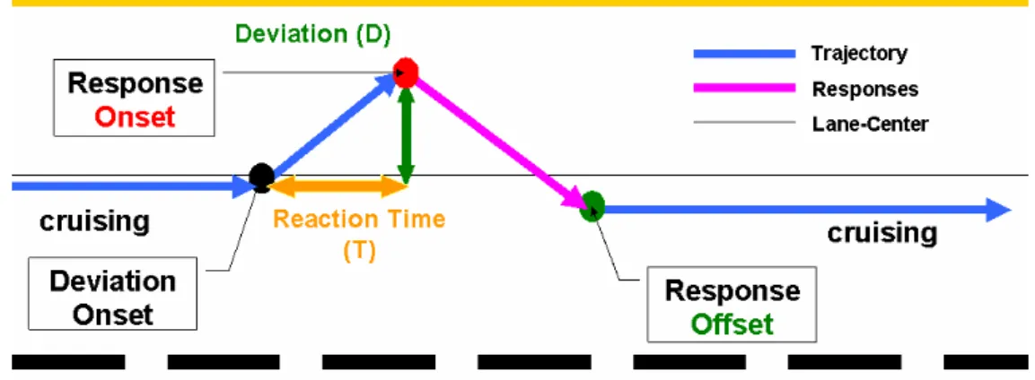
In each 100-min session (Fig. 2-9), 653 deviation events were recorded. Similar to real-world driving experience, the vehicle did not always return to the same cruising position after each compensatory steering maneuver. Therefore, during each drift/response trial, driving error was measured by maximum absolute deviation from the previous cruising position (Fig. 2-10).
Figure 2-9: The illustration of single deviations. (D=c T, c=60).
Figure 2-10: (A) Driving trajectory of a 100-min session. Black dots: deviation onsets. Red dots: response onsets. (B) The driving error of a 100-min session.
Figure 2-11: (A) Sorted trials by driving error (point). (B) Sorted trials by reaction time (sec).
Since the car drifted with constant velocity, the relation between reaction time and the driving error was linear (D=c T, c = 60).
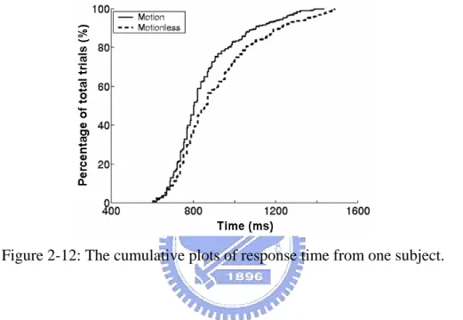
After transformed the driving error into response time, behavior responses were sorted by reaction time, normalized with the total trials, and then plotted as cumulative plot of the response time (showed as Fig.2-12).
Figure 2-12: The cumulative plots of response time from one subject.
The response time and driving error were varied along with drivers’ alertness and drowsiness. We had two equal drowsiness indices: reaction time and the driving error. For instance, when the driver was drowsy, the reaction time between the onset of deviation and steering wheel was increased. On the contrary, when the driver was alter, the response time between the onset of deviation and steering wheel was decrease.
2.5.2. EEG
All the EEG data were analyzed by using the EEGLAB 4.301 (Fig. 2-13). The multi-channel EEG signals were first down sampled (from 500 to 250 Hz) and digital filtered with a linear 1-50Hz FIR pass band filter before the further analysis. Continuous EEG data were segmented into 8.5-s epochs, 2.5 s before and 6 s after the deviation onsets.
Figure 2-13: The flow chart for EEG analysis
The artifacts across all channels were identified and rejected from EEG data using the EEGLAB routines (details see description at
http://www.sccn.ucsd.edu/eeglab/rejtut/tutorialreject.html). Criteria used for artifact rejection included extreme values, abnormal trends (linear drift) and abnormally distributed data (Fig. 2-14).
Figure 2-14: Criteria used for artifact rejection included extreme values, abnormal trends (linear drift) and abnormally distributed data
The preprocessed EEG signals were further separated into independent brain sources using Independent Component Analysis (ICA) as described on the following paragraph.
2.5.2.1. Independent Component Analysis (ICA)
The joint problems of EEG source segregation, identification, and localization are very difficult since the EEG data collected from any point on the human scalp includes activity generated within a large brain area. The problem of determining brain electrical sources from potential patterns recorded on the scalp surface is mathematically underdetermined. Although
the conductivity between the skull and brain is different, the spatial smearing of EEG data by volume conduction does not cause significant time delay and it suggests that the ICA algorithm is suitable for performing blind source separation on EEG data. The ICA methods were extensively applied to blind source separation problem since 1990s (Jutten and Herault, 1991; Cardoso and Souloumiac, 1993; Comon, 1994; Bell and Sejnowski, 1995; Cardoso and Laheld, 1996; Pham, 1997; Girolami, 1998; Lee, 1999). In recent years, subsequent technical reports (Makeig, 1996; Jung, 1998; Jung, 2000; Jung, 2001; Yamazaki, 2003; Meyer-Base, 2003; Naganawa, 2005; Liao, 2005) demonstrated that ICA was a suitable solution to the problem of EEG source segregation, identification, and localization based on the following assumptions: (1) The conduction of the EEG sensors is instantaneous and linear such that the measured mixing signals are linear and the propagation delays are negligible. (2) The signal source of muscle activity, eye, and, cardiac signals are not time locked to the sources of EEG activity which is regarded as reflecting synaptic activity of cortical neurons (Makeig et al., 1996; Jung et al., 1998).
In this study, we attempted to completely separate the twin problems of source identification and source localization by using a generally applicable ICA. Thus, the artifacts including the eye-movement (EOG), eye-blinking, heart-beating (EKG), muscle-movement (EMG), and line noises can be successfully separated from EEG activities. The ICA is a statistical “latent variables” model with generative form:
(1) ) t ( ) t ( As x =
where A is a linear transform called a mixing matrix and the are statistically mutually independent. The ICA model describes how the observed data are generated by a process of mixing the components . The independent components (often abbreviated as ICs) are latent variables, meaning that they cannot be directly observed. Also the mixing matrix A is assumed to be unknown. All we observed are the random variables , and we must estimate
i s i s si i x
both the mixing matrix and the IC’s si using the xi.
Therefore, given time series of the observed data x(t)=
[
x1(t) x2(t) L xN(t)]
T inN-dimension, ICA will find a linear mapping W such that the unmixed signals u(t) are
statically independent. . (2) ) t ( ) t ( Wx u =
Supposed the probability density function of the observations x can be expressed as:
) ( p ) det( ) ( p x = W u , (3)
the learning algorithm can be derived using the maximum likelihood formulation with the log-likelihood function derived as:
∑
= + = N i i i(u ) p log ) det( log ) , ( 1 W W u L , (4)Thus, an effective learning algorithm using natural gradient to maximize the log-likelihood with respect to W gives:
[
I u u]
W W W W W u W L( , ) T ϕ( ) T Δ = − ∂ ∂ ∝ , (5)where the nonlinearity
T N u ) u ( p u ) u ( p ) ( p ) u ( p ) u ( p ) ( p ) ( N N ⎥ ⎥ ⎦ ⎤ ⎢ ⎢ ⎣ ⎡ − − = − = ∂ ∂ ∂ ∂ ∂ ∂ L 1 1 1 u u u u ϕ , (6)
and rescales the gradient, simplifies the learning rule and speeds the convergence considerably. It is difficult to know a priori the parametric density function , which plays an essential role in the learning process. If we choose to approximate the estimated probability density function with an Edgeworth expansion or Gram-Charlier expansion for generalizing the learning rule to sources with either sub- or super-Gaussian distributions, the
W WT
) ( p u
nonlinearity ϕ( u) can be derived as: (7) ⎩ ⎨ ⎧ + − = sources, gaussian -sub for : ) tanh( sources, gaussian -super for : ) tanh( ) ( u u u u u ϕ Then, (8)
[
]
[
]
⎩ ⎨ ⎧ − + − − = Δ gaussian, -sub : ) tanh( gaussian, -super : ) tanh( W uu u u I W uu u u I T T T T WSince there is no general definition for sub- and super-Gaussian sources, we choose
(
(1,1) (-1,1))
2
1 N N
) (
p u = + and for sub- and super-Gaussian, respectively, where ) ( h sec N ) ( p u = (0,1) 2 u
(
μ σ2)
,N is a normal distribution. The learning rules differ in the sign before the tanh function and can be determined using a switching criterion as:
(9)
[
]
⎩ ⎨ ⎧ − = = − − ∝ Δ gaussian, -sub : 1 gaussian, -super : 1 where , ) tanh( i i κ κ W uu u u K I W T T where{
} { }
{
}
(
sec 2( i) i2 tanh( i) i)
, i =signE h u Eu −E u u κ (10)represents the elements of N-dimensional diagonal matrix K. After ICA training, we can
obtain N ICA components u(t) decomposed from the measured N-channel EEG data x(t). In this study, N=30, thus we obtain 30 components from 30 channel signals.
(11) ). ( ) ( ) ( ) ( ) ( ) ( ) ( ) ( 33 33 , 33 33 , 2 33 , 1 2 2 , 33 2 , 2 2 , 1 1 1 , 33 1 , 2 1 , 1 33 2 1 t u w w w t u w w w t u w w w t t x t x t x t ⎥ ⎥ ⎥ ⎥ ⎦ ⎤ ⎢ ⎢ ⎢ ⎢ ⎣ ⎡ + + ⎥ ⎥ ⎥ ⎥ ⎦ ⎤ ⎢ ⎢ ⎢ ⎢ ⎣ ⎡ + ⎥ ⎥ ⎥ ⎥ ⎦ ⎤ ⎢ ⎢ ⎢ ⎢ ⎣ ⎡ = = ⎥ ⎥ ⎥ ⎥ ⎦ ⎤ ⎢ ⎢ ⎢ ⎢ ⎣ ⎡ = M L M M M Wu x
Fig. 2-15 shows an example of the scalp topographies of ICA weighting matrix W
corresponding to each ICA component by projecting each wi,j onto the surface of the scalp,
source) to the EEG channels, e.g., eye activity was projected mainly to frontal sites, and the drowsiness-related potential is on the parietal lobe and occipital lobe, etc. We can observe that most artifacts and channel noises included in EEG recordings are effectively separated into independent components 1 and 7 as shown in Fig. 2-15 and independent components 2 and 10 may be considered as effective “sources” related to drowsiness in the VR-based driving experiment.
Figure 2-15: Scalp topography of ICA decomposition.
2.5.2.2. Time frequency analysis and Event Related Spectral Perturbations
ocessing flow was shown in Fig. 2-16. The time sequence of EEG channel data or ICA activations were subject to Fast Four
(ERSPs)
The pr
ier Transform (FFT) with overlapped moving windows (256 points). Spectra prior to deviation onset were considered as spectral baseline. The mean spectral baselines were converted into dB power and subtracted from spectral
baseline. To reduce random error, spectra in each epoch were smoothed by 3-windows moving-average. The procedure was applied to all the epochs, and their results were then averaged to yield the ERSP image.
The ERSP image mainly showed spectral differences after event, since the baseline spec
.03, here we use 0.01) on ERSP, only
tra prior to event onset had been removed. For instance, the bottom of Figure 2-16 showed that only little or no changes in high frequency band (the lower position the higher frequency) but very significant changes in low frequency band after event. This allowed us to visualize spectral power changes related to the deviations.
After performing bootstrap analysis (usually 0.01 or 0
statistically significant (p<0.01) spectral changes showed in the ERSP images. Non-significant time/frequency points were masked (replaced with zero). Any perturbations in frequency domain became relatively prominent.
Figure 2-16: The flow chart of ERSP analysis.
2.5.3. Clustering
ICs were first selected by observations and large reduced the number of components into around half by rejecting the noisy components (Fig. 2-17). Then, the selected ICs were first classified by the kmeans algorithm into around 10 clusters in terms of the scalp map gradients. These 10 clusters were then grouped into 4 significant clusters by manually removing the non-significant clusters. For guaranteeing these 4 clusters were with the same physiological functionality, we applied the kmeans algorithm again on each of 4 significant clusters based on their power spectral baselines of the components. Finally, components in each IC cluster would have consistent anatomic and functional features (Fig. 2-18).
Figure 2-17: Component selection preceding clustering.
Figure 2-18: The scalp maps for the occipital independent component (IC) cluster. Upper left: the group averaged occipital IC
2.5.4. Statistics
Data were expressed as mean ± SEM unless stated otherwise. (a) To assess the effect of kinesthetic stimulation on distributions of the response time, we used the two sample Kolmogorov-Smirnov tests (K-S test, Matlab statistical toolbox, Mathworks). (c) To compare the baseline alpha power for the fast and slow epochs in two different kinesthetic stimulus conditions, we used the one-way ANOVA and the paired t-test (ttest2, Matlab statistical toolbox, Mathworks). (d) To estimate the significant onset of the alpha suppression, we analyzed the time course of the alpha power as the follows: Changes in alpha power as a function of time was computed by selecting and averaging the amplitude of the ERSP with the frequency from7 to 12 Hz at the occipital component. The significance of the alpha suppression from power spectral baselines was assessed by the statistical bootstrapping (EEGLAB 4.3). The significant onset of the alpha suppression was estimated by the intersection of the time-varying alpha power and the significant level of alpha suppression. All statistical comparisons in this study, a significant level was set at p <0.05.
3. Results
We collected and analyzed 52 driving experiments from 10 subjects, as listed in table 3-1. Each subject completed 4 experiments and each experiment included 1 sessions. First, we compared and presented the influence of kinesthetic stimulation on the behavioral performance. Second, we defined the two different cognitive statuses (fast and slow) according to the distribution of subjects’ response time. Third, we characterized changes of dynamic brain activities from the fast to the slow responses on aspects of the independent component (IC) clusters, the base line power spectrum and the event-related spectral perturbations (ERSPs) under different kinesthetic conditions (motion and motionless). The following paragraphs showed detailed results.
Table 3-1: Subject list Platform mode motion motionless Subject 1 06/10/20 07/01/05 07/03/12 06/10/28 06/11/21 Subject 2 06/10/27 07/01/15 07/01/24 06/11/10 07/01/19 07/01/31 07/03/22 Subject 3 06/11/22 06/12/07 07/01/04 07/01/16 06/11/30 06/12/21 Subject 4 06/12/04 06/12/20 06/12/27 06/12/13 07/01/29 Subject 5 06/12/18 06/12/26 07/01/12 07/01/02 07/01/17 Subject 6 06/12/19 06/12/29 07/01/16 07/01/31 07/01/24 07/02/07 Subject 7 06/12/20 07/01/03 06/12/25 07/01/17 Subject 8 07/01/26 07/02/02 07/02/06 07/02/05 07/02/08 Subject 9 07/01/26 07/02/09 07/02/05 07/03/25 Subject 10 07/02/09 07/03/13 07/03/08 07/03/07 07/03/21
3.1. Behavioral performance
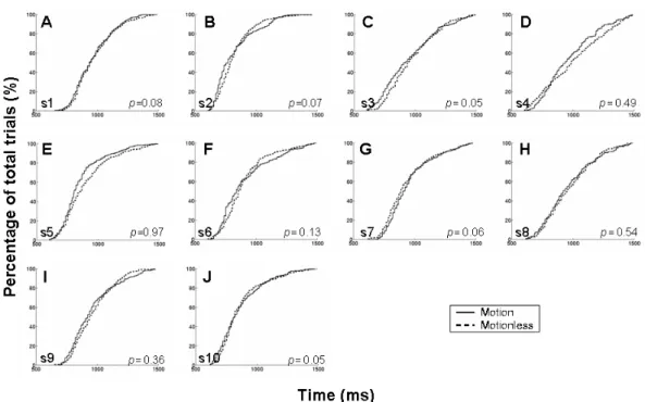
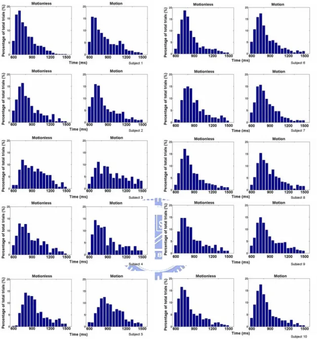
All subjects’ response time were ranged from 600 ms to 1500 ms (Fig. 3-1). No clear and statistically significant differences displayed on the cumulative percentage plots and the distribution of response time between the motion and motionless conditions in each subject (Fig. 3-1). Ten subjects’ response time histogram of motionless and motion sessions were shown in Fig. 3-2. All subjects exhibited fast (shorter response time) and slow (longer response time) performance period and their distribution did not showed statistically significant differences between the motion and motionless sessions (Fig. 3-3). The above results suggested that the kinesthetic stimulus had no effects on the global and local distribution of behavioral performance. The Fig. 3-4 and 3-5 showed ten subjects’ response time histograms of fast and slow epochs in the motion and motionless sessions.
Figure 3-1: The cumulative percentage plots of the response time from ten subjects. (A-J): motionless groups (dash line); motion groups (solid line). Note, no
Figure 3-2: The same data as in the Fig. 3-1 but displayed as the response time
histograms. The motionless groups (left column) and the motion groups (right column). Note no subjects showed apparently differences in distributions of the response
Figure 3-3: The cumulative percentage plots (A) of the response time and their corresponded response histograms (B-E) of the subject 5. Trials were equally divided into three parts according to the response time (0.6 -1.5 sec). Trials with response time from 0.6 to 0.9 sec were selected as the fast groups (a) and trials with response time from 1.2 to 1.5 sec were as the slow groups (b). The response time histograms of fast and slow groups were showed in (B-E). (B, D): the motionless groups; (C, E): the motion groups. Note: no apparently effects of kinesthetic stimulus on the distribution of the response time histograms in the fast or slow groups.
Figure 3-4: The response time histogram of fast and slow groups of 4 subjects. The motionless groups (left column); the motion groups (right column).
Figure 3-5: The response time histogram of fast and slow groups of 6 subjects. The motionless groups (left column); the motion groups (right column).
3.2. Independent Component (IC) clustering
Components were first selected and clustered by the correlation between the scalp map gradients and their power spectral baselines across a session and ten subjects. The grand mean scalp maps of a session (10 subjects) for four ICs were showed in Fig 3-6 to Fig 3-9. The occipital clustering was included ICs nearly from all sessions (10 sessions) and subjects and the central, left mu and right mu clustering were include ICs with the range from 5 to 8 of all sessions and subjects. The ICs in the same cluster were showed similar power spectral baselines and event-related spectral perturbations (ERSPs) changes. The Fig. 3-10 showed the grand mean power spectral baselines and the averaged scalp maps of the four IC clusters.
Figure 3-6; The scalp maps for the occipital independent component (IC) cluster of 10 motionless (Left columns) and 10 motion (right columns) sessions across 10 subjects. Upper panels: the group averaged occipital IC of the motionless and motion groups. Lower panels: scalp maps for the occipital IC of the motionless and motion groups from 10 subjects.
Figure 3-7: The scalp maps for the left Mu rhythm IC cluster of 8 motionless and 8 motion sessions across 10 subjects. Panels as Fig. 3-6.
Figure 3-8: The scalp maps for the right Mu rhythm IC cluster of 7 motionless and 6 motion sessions across 10 subjects. Panels as Fig. 3-6.
Figure 3-9: The scalp maps for the Central IC cluster of 5 motionless and 8 motion sessions across 10 subjects. Panels as Fig. 3-6.
Figure 3-10: showed the grand mean power spectral baselines and the averaged scalp maps of the four IC clusters. The occipital (A, E); central (B, F); left Mu (C, G) and right Mu (D, H); ICs. The mean (solid lines) power spectra.
3.3. Tonic brain dynamics at a large time scale
The following paragraphs showed effects of kinesthetic stimulation on changes of power spectral baselines in four ICs at a large time scale within the individual subject and across ten subjects for fast and slow epochs.
3.3.1. Within subjects phenomena
Fig. 3-11 showed the averaged power spectral baselines in the occipital component of the subject 5 for fast and slow epochs from the motionless and motion conditions. Under the motionless, the mean baseline power spectrum was statistically significant larger at the frequency from 4-12 Hz in the slow epochs than those in the fast epochs (Fig. 3-11). The similar changes on the tonic activity were also found in the motion condition. Comparing with the motionless, the difference nearly the alpha band between these two averaged power spectral baselines was larger when the motion platform was enabled. Similar differences on the tonic brain activities between the motionless and motion sessions were also demonstrated
Some subjects (as shown in Fig 3-12 to 3-14) showed similar increases nearly the beta band from fast to slow epochs in the motion and/or motionless conditions.
Figure 3-11: Single subject’s results. Average power spectral baselines of two groups of epochs under motionless and motion conditions. He mean (solid lines) power spectra (± SEM: dashed lines) of the fast epochs (blue traces) and the slow epochs (black traces). Note the significant power increases (slow minus fast) at the alpha band in the occipital ICs. The power increase was larger in the motion sessions than that in the motionless session.
Figure 3-12: The averaged baseline power spectra of 2 subjects. The fast epochs (blue traces) and the slow epochs (black traces).
Figure 3-13: The averaged baseline power spectra of 4 subjects. The fast epochs (blue traces) and the slow epochs (black traces).
Figure 3-14: The averaged baseline power spectra of 4 subjects. The fast epochs (blue traces) and the slow epochs (black traces).
Figure 3-15: The averaged baseline alpha power of ten subjects. Note no apparently differences between the motion and motionless sessions in the fast response condition. But, the significant power increases were showed in motion sessions for the slow responses. Hollow bars: the motionless sessions; shaded bars: the motion sessions.
For characterizing effects of the kinesthetic stimulation on detail changes of the alpha power from fast to slow epochs in each subject, the power at the alpha band were selected and averaged from the baseline power spectra, as shown in Fig. 3-15. The mean alpha power of the fast epochs between the motionless and motion sessions appeared comparable in each subject. The mean alpha power of individual subjects was significantly increased in slow epochs and further, such increase was over enhanced by the kinesthetic stimulation (Fig. 3-15). Values of ten subjects’ averaged baseline alpha power in the occipital ICs were shown in table 3-2.
The above changes on the baseline power spectra at the alpha band were not found in the central, left mu or right mu ICs (Fig. 3-11).
3.3.2. Cross subject consistency
The grand mean of the power spectral baselines of four ICs for the fast and slow epochs in motion and motionless groups were shown in Fig. 3-16. Despite variations in EEG recordings across different sessions and subjects, grand mean baseline power spectra of occipital IC showed statistically significant increase at the alpha band (p<0.01 shown in figure 3-17, p<0.01 shown in figure 3-18) in the slow epochs. Furthermore, the kinesthetic stimulus significantly increased the difference of the baseline alpha power between the fast and slow epochs (left bars vs. right bars, p<0.01, Figure 3-18). Such increased differences on baseline alpha power were only related to the over enhanced the tonic power at alpha band at the slow epochs (fast: hollow bar vs. shaded bar, p=0.8; slow: hollow bar vs. shaded bar, p<0.01). The summary of the averaged power spectral baseline at alpha band of the occipital IC were shown in table 3-3.
Figure 3-16: The grand mean (±SEM) baseline power spectra of two groups of epochs for four ICs in motionless (Left column, n=10) and motion (right column, n=10) sessions. The occipital (A, E); central (B, F); right Mu (C, G) and left Mu (D, H); ICs. The mean (solid lines) power spectra (± SEM: dash lines) of the fast epochs (blue traces) and the slow epochs (black traces). Note compared with the other ICs, the significant power increases (slow minus fast) at the alpha band were only displayed in the occipital ICs. The power increase was larger in the motion sessions than that in the motionless session. Insets: the group averaged scalp maps.
The above changes on the baseline alpha power were only localized at the occipital IC. No apparently differences were found on the tonic power around 8-12 Hz between the fast and slow epochs in either motionless or motion groups (Fig.3-16).
Figure 3-17: The effects of kinesthetic stimulus and cognitive status on the averaged baseline alpha power from ten subjects. Note the effects of kinesthetic stimulus boosted the increase of baseline alpha power in the slow epochs (**: p <0.01; ##:
p<0.01).
Figure 3-18: The kinesthetic stimulus significantly increased the difference of the baseline alpha power between the fast and slow epochs (**: p<0.01).
Table 3-2: The mean baseline alpha power for ten subjects
3.4. Event-Related Spectral Perturbations (ERSPs)
Effects of kinesthetic stimulation and changes of cognitive status on the phasic dynamics at a small time scale in four ICs (occipital, left mu and right mu and central components) were shown in the following paragraphs.
3.4.1. The occipital component
Fig. 3-19 displayed ERSP images showing mean log power changes following car drifted in fast and slow epochs for an occipital IC of subject 5 in motion and motionless conditions. The mean ERSP for fast epochs (Fig. 3-19B and 3-19D) showed that mean power in the alpha band (near 10 Hz) suppressed following deviation onset (phasic changes). Comparing with the motion session, the phasic decrease followed the car drifted was weaker for the fast epochs in the motion session. For the epochs of fast performance in the motionless session, the suppressed alpha band was slightly increased around the response offset.
Figure 3-19: The ERSP images of occipital component for fast (B, D) and slow (A, C) epochs in motionless and motion session of subject 5. Pink dashed lines: The deviation onset. Blue dashed lines: the mean of reaction time. The right column: the group averaged scalp maps of the occipital component for motionless (top) and the motion session (bottom). Color bar: power of ERSPs. Note the alpha power was suppressed briefly after the deviation onset and the latency for the alpha suppression was related to the response time.
In slow epochs, the suppression in alpha power before the response onset was prolonged. Phasic changes in power around the beta band were smaller than in the alpha band. The latency of alpha suppression was correlated with reaction time. Furthermore, the response latency of the alpha suppression was further delayed in the motion session (Fig. 3-19). ERSP images of other nine subjects showed in Fig. 3-20 to 3-23.
Figure 3-20: The ERSPs of the occipital component for fast (B, D) and slow (A, C) epochs in motionless (A, B) and motion (C, D) sessions of subject 1 and 2.
Figure 3-21: The ERSPs of the occipital component for fast (B, D) and slow (A, C) epochs in motionless (A, B) and motion (C, D) sessions of subject 3, 4, and 6.
Figure 3-22: The ERSPs of the occipital component for fast (B, D) and slow (A, C) epochs in motionless (A, B) and motion (C, D) sessions of subject 7, 8, and 9.
Figure 3-23: The ERSPs of the occipital components for fast (B, D) and slow (A, C) epochs in motionless (A, B) and motion (C, D) sessions of subject 10.
Figure 3-24: The grand mean of ERSP images of occipital component for fast (B, D) and slow (A, C) epochs in motionless and motion sessions across ten subjects. Panels as Fig.3-19.
Fig. 3-24 showed the grand mean of ERSP images of occipital component for fast and slow epochs in motionless and motion sessions from ten subjects. Power spectra in the
occipital cluster showed slightly broader phasic changes after the deviation onset, with peaks near 10 Hz in slow epochs (Fig. 3-24A and Fig. 3-24C). Fig. 3-25 showed, the grand mean percentage of the 5 sec period after the deviation onset exhibiting significant (p<0.01) phasic changes for each frequency from ten subjects. This prevalence measurement can be interpreted as the probability of a significant decrease in post-response power, across subjects. Phasic changes in fast epochs were less frequent (occupying on average around 40 % of the post-deviation periods) than in slow epochs (on average ~60 %). In motionless session, the changes at the alpha band power displayed a slight downward frequency shift in the alpha peak (Fig. 3-25A, middle panel). With the kinesthetic stimulation, the frequency range of phasic increases in slow epochs was wider than that in the fast epochs (25 Hz vs. 20 Hz).
Figure 3-25: Percentage of the 0-5 sec post-deviation epochs with significant (p<0.01) phasic (post- minus pre-deviation) power decreases, averaged across ten subjects’ occipital ICs in motionless (A) and motion session (B). Blue traces: fast epochs. Black traces: slow epochs.
3.4.2. The motor component
The mean ERSPs for fast epochs (Fig. 3-26B and Fig. 3-26D) showed phasically decreased activity in the (8-12 Hz) alpha and (15-25 Hz) beta band power. The ERSP images for slow epochs (Fig. 3-26A and Fig. 3-26C) showed a prolonged decrease in EEG activity below the 12 Hz after the deviation onsets. The onset of the beta suppression showed a slightly earlier than the onset of the alpha band. For epochs with slow performance, the latency of the alpha suppression was clearly shorter in the motion session than that in the motionless session. Fig. 3-27 and 3-28 showed the ERSP images of right mu components in individual subjects.
Figure 3-26: The ERSP images of right mu component for fast (B, D) and slow (A, C) epochs in motionless and motion session of subject 5. Panels as Fig. 3-19. Note: the onset for the alpha suppression for the slow epochs was earlier in the motion session than that in the motionless session.
Figure 3-27: The ERSP images of right mu component for fast (B, D) and slow (A, C) epochs in motionless and motion session of subject 1, 3, and 6. Panels as Fig. 3-19.
Figure 3-28: The ERSP images of right mu component for fast (B, D) and slow (A, C) epochs in motionless and motion session of subject 7 and 9. Panels as Fig. 3-19.
Similar spectra changes at the alpha and beta band following the deviation onset were demonstrated in the ERSPs for motor ICs (left and right mu components) averaged across ten subjects showed in Fig. 3-29. In the fast epochs, the phasic activity changes were significantly weaker in the right mu component when the motion platform was disabled.
Figure 3-29: The grand mean of ERSP images of left and right mu component for fast (B, D) and slow (A, C) epochs in motionless and motion session from ten subjects. Panels as Fig. 3-19.
No apparently difference in mean prevalence of the power decrease between the fast and slow epochs (fast: ~40- 50%; slow: ~40-50%). In slow epochs, changes at frequencies around 5Hz were more frequent (occupying on average about 45 % of the post-response periods) than in fast epochs (on average lower than 10 %).
Figure 3-30: Percentage of the 0-5 sec post-deviation epochs with significant (p<0.01) phasic (post- minus pre-deviation) power decreases, averaged across ten subjects’ left (n=6) and right (n=8) mu components in motionless (A, C) and motion session (B, D). Blue traces: fast epochs. Black traces: slow epochs.
3.4.3. The central component
Fig. 3-31 showed the ERSPs of the central ICs of subject 5. For the central ICs, there were no apparently phasic activity changes around the alpha and bands. For the fast epochs, spectra below 10 Hz showed a transient and strong power increases following the deviation onset in the motionless session. However, a significant and sustained power decreases at frequencies below 10 Hz were observed in the slow epochs during the motion session.
Figure 3-31: The ERSP images of central IC for fast (B, D) and slow (A, C) epochs in motionless and motion session of subject 5. Panels as Fig. 3-19. Note: the clear power increases below the 10 Hz showed briefly after the deviation onset in the fast epochs when the motion platform was disabled. A sustained power decreased around the response onset showed for the slow epochs when the motion platform was enabled.
Fig. 3-32 showed the grand mean of ERSPs of central components averaged across ten subjects. For the large variations in individual ERSP across sessions and subjects, the grand mean of ERSP only showed slightly increased power at frequencies below (Fig. 3-32) or around (Fig. 3-32A)10Hz after the car drifted. The lightly power decreases around the alpha band were also exhibited in the grand mean of the response-locked ERSPs.
Figure 3-32: The grand mean of ERSPs of the central IC for fast (B, D) and slow (A, C) epochs in motionless and motion sessions from ten subjects. Panels as Fig. 3-18.
3.5. The onset of the alpha suppression
Fig. 3-33 showed the spectrotemporal traces of the alpha band power at the occipital components. In the slow epochs, the onset of the alpha suppression was significantly delayed than in the fast epochs. The latency of the alpha suppression was further delayed during the motion sessions (Fig. 3-33B). For fast epochs, there were no significant differences on the onset of alpha decreases between the motionless and motion sessions. In the mu ICs, changes of response performance had an effect on decrease of alpha band power by delaying its onset. However, comparing with the occipital components, effects of kinesthetic stimulation on the
onset of the alpha suppression were totally different in the mu components. Specifically, the onset of the alpha decrease in the motor components was significantly shortened both in fast and slow epochs (left mu: 3-34A vs. 3-34B; right mu: 3-34C vs. 3-34D, fig. 3-34) when the motion platform was enabled.
Figure 3-33: Averaged time courses of the alpha band for fast (black traces) and slow (blue traces) epochs in motionless (A) and motion (B) sessions across ten subjects. Dash lines: the significant values (p<0.01) of fast (black traces) and slow (blue traces) epochs by bootstrap. Arrows indicate the significant onset of the alpha suppression for the fast and slow epochs. Insets: the group averaged scalp maps of the occipital components and the ICA weightings. Note the mean onset of alpha decrease was delayed in the slow epochs and the kinesthetic stimulation further delayed the latency of the alpha suppression.
Figure 3-34: Averaged time courses of the alpha band at the mu components (Left column: left mu; right column: right mu) in fast (black traces) and slow (blue traces) epochs during motionless (A) and motion (B) sessions across ten subjects. Panels as Fig. 3-33. Note the kinesthetic stimulation shortened the latency of the alpha suppression for both fast and slow epochs. (**: p<0.01)
Figure 3-35: Effects of kinesthetic stimulation and changes of response performance on the mean latency of alpha suppressions at the occipital (A) and mu ICs (B: left; C: right) in both fast and slow epochs (**: p <0.01).
Table 3-4: The averaged onset of the alpha suppression in the occipital components.
Table 3-5: The averaged onset of the alpha suppression in the right mu components.
4. Discussion
In this study, we demonstrated that the level of driver’s drowsiness can be affected by the kinesthetic stimuli based on the 3 dimensional surrounded virtual reality scene combined with the six degree motion platform, the independent component analysis (ICA) and time-spectral analysis to explore the fluctuations in spectral dynamics of maximally independent EEG activities from alter to drowsy with or without the enabling of the motion platform.
4.1. Effects of drowsiness on long-term tonic variations
For both the motion and motionless sessions, the tonic increases in power spectral baselines from fast to slow epochs in the occipital components were consistently observed across subjects. Similar changes on the tonic brain dynamics from low- to high-error trials have been observed in a compensatory simulated driving task (Huang et al., 2005). In that study, the tonic alpha power also increased at the occipital components during the period of poor behavioral performance was observed in the IC clusters originating in the lateral occipital cortex. During drowsy, as indexed by the behavioral performance drop-offs, tonic scalp EEG power has been found to be higher on average than during alert or awake although most studies also observed tonic increases at the theta power (Saroj and Ashley, 2002; Campagne et al., 2004). Another experiment in our laboratory characterized details changes of EEG dynamics from alert, light drowsiness to deep drowsiness under motionless condition. Results suggested that the alpha activities increased either in a monotonic or non-monotonic pattern while the theta band power increased linearly and slowly from the drowsy onset to the deep drowsiness. The strength of alpha power was larger than theta waves during the period of light drowsy whereas the power of theta band was significant larger than the alpha band power in the period of deep drowsiness. In this study, the tonic increases of baseline band power for the slow epochs were not only significant larger at alpha band, but also the theta-