應用於行動式視訊裝置之預設位元平面比對之嵌入式編解碼器

國立交通大學

電機學院 IC 設計產業研發碩士班

碩 士 論 文

應用於行動式視訊裝置之預設位元平面比對之嵌入式

編解碼器

An Embedded Codec Based on Predefined Bitplanes

Comparison Coding for Mobile Video Applications

學生 ： 林建辰

指導教授 ： 李鎮宜 教授

應用於行動式視訊裝置之預設位元平面比對之嵌入式

編解碼器

An Embedded Codec Based on Predefined Bitplanes

Comparison Coding for Mobile Video Applications

研 究 生：林建辰 Student：Chien-Cheng Lin

指導教授：李鎮宜 Advisor：Dr. Chen-Yi Lee

國 立 交 通 大 學

電機學院 IC 設計產業研發碩士班

碩 士 論 文

A Thesis

Submitted to College of Electrical and Computer Engineering National Chiao Tung University

in Partial Fulfillment of the Requirements for the Degree of

Master in

Industrial Technology R&D Master Program on IC Design

June 2010

Hsinchu, Taiwan, Republic of China

應用於行動式視訊裝置之預設位元平面比對之嵌入式

編解碼器

學生：林建辰 指導教授：李鎮宜 教授

國立交通大學電機學院產業研發碩士班

摘要

An Embedded Codec Based on Predefined Bitplanes

Comparison Coding for Mobile Video Applications

Student: Chien-Cheng Lin Advisor: Dr. Chen-Yi Lee

Industrial Technology R & D Master Program of

Electrical and Computer Engineering College

National Chiao Tung University

ABSTRACT

For mobile video applications, the required storage and bandwidth of frame memory play crucial roles. Reducing the accesses and the size of frame memory can decrease area, cost, as well as power consumption. Most of video compressions indicate that higher complexity can reach better performance. However, the lower complexity algorithm is easier to be embedded into H.264 decoder. In this paper, a novel embedded lossy compression scheme is proposed. It compresses a 4x2 size block into 32 bits segment. The compression ratio (CR) is fixed at 2. The PSNR loss is 1.89~3.45dB. A pipelined architecture has been proposed to realize both compressor and decompressor in 2 cycles and 1 cycle respectively. This cost-effective solution requires gate count of 4.9k and power consumption of 244uW in 90nm standard CMOS process.

誌

謝

Index

CHAPTER 1 INTRODUCTION ... 1 

1.1  MOTIVATION ... 1 

1.2  THESIS ORGANIZATION ... 2 

CHAPTER 2 PREVIOUS WORKS ... 3 

2.1  LOSSLESS EMBEDDED COMPRESSION ALGORITHM ... 3 

2.2  LOSSY EMBEDDED COMPRESSION ALGORITHM ... 3 

2.2.1  Block Truncation Coding (BTC) Compression ... 4 

2.2.2  Block Truncation Coding using a set of predefined bitplanes ... 6 

2.2.3  Bitplane Truncation Coding ... 9 

2.3  SUMMARY ... 10 

CHAPTER 3 PROPOSED ALGORITHM ... 11 

3.1  ALGORITHM OF EMBEDDED COMPRESSION ... 11 

3.1.1  Pixel Truncation ... 12 

3.1.2  Selective Start Plane ... 13 

3.1.3  Compensation ... 14 

3.1.4  Predefined Bitplanes Comparison ... 15 

3.2  SIMULATION RESULTS ... 16 

CHAPTER 4 PROPOSED ARCHITECTURE ... 19 

4.1  ARCHITECTURE OF COMPRESSOR ... 19 

4.1.1  Architecture of Pixel Truncation ... 19 

4.1.2  Architecture of Selective Start Plane ... 20 

4.1.4  Architecture of Predefined Bitplanes Comparison ... 21 

4.1.5  Data Packing ... 22 

4.2  ARCHITECTURE OF DECOMPRESSOR ... 23 

4.2.1  Data Rearrange ... 23 

4.3  DESIGN IMPLEMENTATION AND VERIFICATION ... 23 

4.3.1  Design Implementation ... 24 

4.3.2  Design Verification ... 24 

CHAPTER 5 SYSTEM INTEGRATION ... 26 

5.1  SYSTEM ANALYSIS ... 26 

5.2  ACCESS ANALYSIS ... 30 

5.2.1  Write Reduction ... 32 

5.2.2  Read Reduction ... 32 

5.3  PROCESSING CYCLE ANALYSIS ... 34 

5.3.1  Access Reduction Ratio ... 35 

5.3.2  Simulation Result on Power Reduction ... 35 

CHAPTER 6 CONCLUSION AND FUTURE WORKS ... 37 

6.1  CONCLUSION ... 37 

6.2  FUTURE WORK ... 37 

Figures List

FIG.1 THE COMPRESSION FLOW OF BLOCK TRUNCATION CODING ... 4 

FIG.2 COMPRESSED 26-BIT SEGMENT FORMAT OF BLOCK TRUNCATION CODING ... 4 

FIG.3 THE COMPRESSION FLOW OF IMPROVING BLOCK TRUNCATION CODING ... 6 

FIG.4 COMPRESSED 16-BIT SEGMENT FORMAT OF IMPROVING BLOCK TRUNCATION CODING ... 6 

FIG.5 64 CLASSES OF LINE AND EDGE BITPLANES (REVERSE VERSIONS NOT SHOWN) ... 7 

FIG.6 THE COMPRESSION FLOW OF BLOCK TRUNCATION CODING USING A SET OF PREDEFINED BITPLANES ... 8 

FIG.7 TEN BASIC BITPLANES CAN BE EXTEND THE THIRTY-TWO BITPLANES ... 8 

FIG.8 COMPRESSED 16-BIT SEGMENT FORMAT OF BLOCK TRUNCATION CODING USING A SET OF PREDEFINED BITPLANES ... 8 

FIG.9 COMPRESSION FLOW OF THE PROPOSED ALGORITHM ... 11 

FIG.10 COMPRESSED 32-BIT SEGMENT FORMAT ... 12 

FIG.11FLOWCHART OF THE PIXEL TRUNCATION ... 13 

FIG.12FLOWCHART OF THE SELECTIVE START PLANE ... 14 

FIG.13FLOWCHART OF THE ROUNDING ... 15 

FIG.14AN EXAMPLE OF PARTITIONING 4X2 BLOCK ... 16 

FIG.15PSNR AND PSNRLOSS FOR ALL CIF SEQUENCES ... 17 

FIG.16DRIFT EFFECT FOR MOBILE_QP28 ... 17 

FIG.17DRIFT EFFECT WITH DIFFERENT QP AND GOP ... 18 

FIG.18THE PIPELINED ARCHITECTURE OF COMPRESSOR DESIGN ... 19 

FIG.19ARCHITECTURE OF PIXEL TRUNCATION ... 20 

FIG.20ARCHITECTURE OF SELECTIVE START PLANE ... 20 

FIG.22ARCHITECTURE OF PREDEFINED BITPLANES COMPARISON ... 22 

FIG.23ARCHITECTURE OF DATA PACKING ... 22 

FIG.24THE PIPELINE ARCHITECTURE OF DECOMPRESSOR ... 23 

FIG.25ARCHITECTURE OF DATA REARRANGE ... 23 

FIG.26THE VERIFICATION FLOW ... 25 

FIG.27THE BLOCK DIAGRAM OF THE OVERALL H.264 DECODER SYSTEM ... 26 

FIG.28THE SYSTEM INTERFACE DESIGN FOR EMBEDDED CODEC ... 27 

FIG.29AN EXAMPLE OF OVERHEAD PROBLEM ... 28 

FIG.30THE FLOW OF EC ACCESSES ... 29 

FIG.31THE BLOCK DIAGRAM OF COWARE SYSTEM ... 30 

FIG.32BLOCK DIAGRAM IN COWARE SYSTEM ... 31 

FIG.33EMBEDDED COMPRESSOR WAVEFORM OVER COWARE SYSTEM ... 31 

FIG.34DATA ACCESS TRACE ... 32 

FIG.35POWER ANALYSIS ON HD1080/720@150MHZ ... 36 

Tables List

TABLE1THREE GROUP OF EIGHT PREDEFINED BITPLANES ... 15 

TABLE2SUMMARY OF THE HARDWARE IMPLEMENTATION ... 24 

TABLE3OVERHEAD WITH BLOCK GRID FOR SIX SEQUENCES ... 29 

TABLE4ALL CASES OF READ ACCESS REQUIRED BY MC WITH/WITHOUT EC ... 33 

Chapter 1

Introduction

1.1 Motivation

A video coding standard achieves high compression efficiency such as MPEG-2, MPEG-4, H263, H.264 [1] [2], and so forth. For H.264 decoder [3], at least one previous frame is stored in frame memory to generate a predicted frame. Accordingly, Motion Compensation (MC) and Deblocking Filter demands a huge amount of data access between off-chip memory devices and the video decoder chip. Thereby, data access dominates the power consumption of H.264 decoder.

For mobile video devices, one major issue is the limited power supply from battery. Even though many low power approaches, such as energy recycle, sub-threshold cell, and et al, can reduce a lot of power in chip. However, data transferring also consumes a lot of power. Therefore, for hardware design, it is important reducing access times.

As aforementioned descriptions, our improvement aspects conclude: 1) reducing access times, and 2) reducing the size of frame memory. Moreover, Embedded Compression (EC) can deal with the above two improvement aspects. However, data compression is not only lossless compression but also lossy compression. Lossless compression can guarantee no quality loss, but variable length of the compressed data caused irreducible frame memory size. On the contrary, lossy compression with the fixed CR can guarantee the reduction of frame memory size. Consequently, it is important to design an applicable a lossy EC.

1.2 Thesis Organization

The rest of this paper is organized as follows. Chapter 2 introduces data compression and previous works. In Chapter 3, a novel algorithm is briefly described. The hardware architecture suitable for mobile video applications is given in Chapter 4. The design implementation and verification are shown in 4.3. We discuss the integration with an available H.264 decoder [3] and the experimental results respectively in Chapter 5. Finally, the conclusions and future work will be given in Chapter 6.

Chapter 2

Previous Works

In general, embedded compression algorithms can be categorized into two fundamental groups: lossless embedded compression algorithms and lossy embedded compression algorithms. First, we briefly explain the existing lossless embedded compression algorithms. Second, we introduce the existing lossy embedded compression algorithms. Finally, we summarize merits and drawbacks of two fundamental groups of embedded compression algorithms.

2.1 Lossless Embedded Compression Algorithm

Lossless embedded compression algorithms [4] can guarantee no quality distortion of video sequences. Moreover, it has no error propagation problem in H.264 decoder. However, after lossless compressing, the compressed data is variable length. Therefore, existing lossless approaches are not suitable for frame compression because their primary purpose is high coding efficiency rather than low latency, low visual quality distortion, low computation complexity, and high random accessibility.

2.2 Lossy Embedded Compression Algorithm

Lossy compression algorithms, comparing with lossless compression algorithms, accomplish the fixed compression ratio (CR). Several lossy embedded compression algorithms have been proposed, such as Block Truncation Coding (BTC) [5], improving

BTC by line and edge information and adaptive bitplane selection [6], BTC using a set of predefined bitplanes [7], Modified Hadamard Transform (MHT) and quantization of Colomb-Rice Coding [8], DCT and Modified Bitplane Zonal Coding (MBZC) [9], and et al.

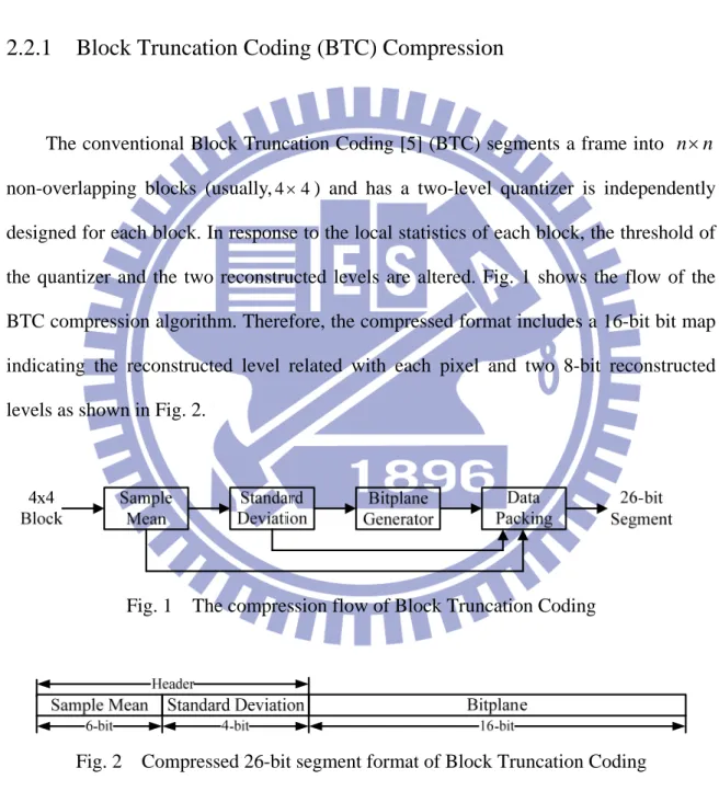
2.2.1 Block Truncation Coding (BTC) Compression

The conventional Block Truncation Coding [5] (BTC) segments a frame into n n×

non-overlapping blocks (usually,4×4) and has a two-level quantizer is independently designed for each block. In response to the local statistics of each block, the threshold of the quantizer and the two reconstructed levels are altered. Fig. 1 shows the flow of the BTC compression algorithm. Therefore, the compressed format includes a 16-bit bit map indicating the reconstructed level related with each pixel and two 8-bit reconstructed levels as shown in Fig. 2.

Fig. 1 The compression flow of Block Truncation Coding

Fig. 2 Compressed 26-bit segment format of Block Truncation Coding

A two-level quantizer is designed to preserve the mean and variance of a block. First, a frame is divided into non-overlapping n n× blocks. Let 2

m=n , let X X₁, ₂,",X_m be

the pixel values of a block. The sample mean (α) and absolute moment (β ) are given in (1) and (2). 1 1 m i i x m = α =

∑

∑

The sample mean and absolute moment are preserved. By taking the mean (α) as the threshold, the two reconstructed levels, a and b are given in (3) and (4).

2 m a p β α = − (3) 2 m b q β α = − (4)

where p is number of smaller than the mean and q is the number of greater than or equal to the mean. Because BTC is a minimum mean square error (MMSE), the reconstructed level a can be simplified as (5).

' i X s X s_i' 1 i i x a p∀ <α =

∑

Similarly, b also becomes as (6).

1 i i x b q∀ ≥α =

∑

As above equations, the additions and comparisons are required. Therefore, in hardware implementation, BTC is very simple. The decoder is even simpler. However, the quality loss of BTC is not suitable to be embedded into the H.264 decoder. Therefore, we can learn the proposed architecture. Moreover, in H.264 decoder, the simpler decoder also provides higher random accessibility.

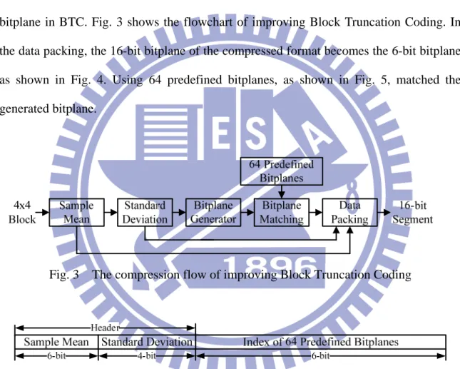
2.2.2 Block Truncation Coding using a set of predefined bitplanes

As aforementioned BTC, the encoder generated two reconstructed levels and the bitplane. For a block, the bitplane can result 65536 (= ) possible number of bitplanes. For the limited data budget, the bitplane occupied 16-bit of the compressed format. Thus,

4×4 216

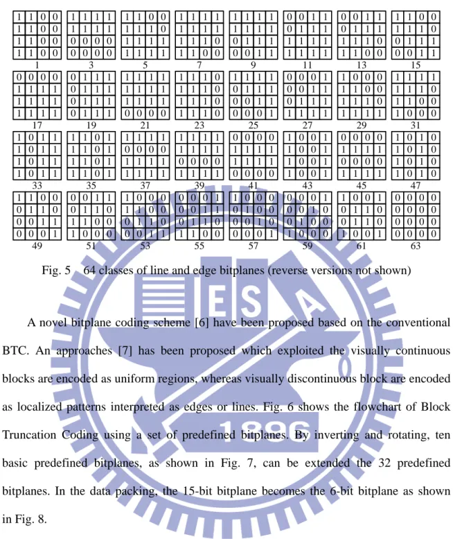
[6] have been proposed an approach to reduce the bit number of the bitplane in BTC. Fig. 3 shows the flowchart of improving Block Truncation Coding. In the data packing, the 16-bit bitplane of the compressed format becomes the 6-bit bitplane as shown in Fig. 4. Using 64 predefined bitplanes, as shown in Fig. 5, matched the generated bitplane.

Fig. 3 The compression flow of improving Block Truncation Coding

Fig. 4 Compressed 16-bit segment format of improving Block Truncation Coding

1 1 1 0 0 1 1 0 0 1 1 0 0 1 1 0 0 3 1 1 1 1 1 1 1 1 0 0 0 0 0 0 0 0 5 1 1 0 0 1 1 1 0 1 1 1 1 1 1 1 1 7 1 1 1 1 1 1 1 1 1 1 1 0 1 1 0 0 9 1 1 1 1 1 1 1 1 0 1 1 1 0 0 1 1 11 0 0 1 1 0 1 1 1 1 1 1 1 1 1 1 1 13 0 0 1 1 0 1 1 1 1 1 1 0 1 1 0 0 15 1 1 0 0 1 1 1 0 0 1 1 1 0 0 1 1 17 0 0 0 0 1 1 1 1 1 1 1 1 1 1 1 1 19 0 1 1 1 0 1 1 1 0 1 1 1 0 1 1 1 21 1 1 1 1 1 1 1 1 1 1 1 1 0 0 0 0 23 1 1 1 0 1 1 1 0 1 1 1 0 1 1 1 0 25 1 1 1 1 0 1 1 1 0 0 1 1 0 0 0 1 27 0 0 0 1 0 0 1 1 0 1 1 1 1 1 1 1 29 1 0 0 0 1 1 0 0 1 1 1 0 1 1 1 1 31 1 1 1 1 1 1 1 0 1 1 0 0 1 0 0 0 33 1 0 1 1 1 0 1 1 1 0 1 1 1 0 1 1 35 1 1 0 1 1 1 0 1 1 1 0 1 1 1 0 1 37 1 1 1 1 0 0 0 0 1 1 1 1 1 1 1 1 39 1 1 1 1 1 1 1 1 0 0 0 0 1 1 1 1 41 0 0 0 0 1 1 1 1 1 1 1 1 0 0 0 0 43 1 0 0 1 1 0 0 1 1 0 0 1 1 0 0 1 45 0 0 0 0 1 1 1 1 0 0 0 0 1 1 1 1 47 1 0 1 0 1 0 1 0 1 0 1 0 1 0 1 0 49 1 1 0 0 0 1 1 0 0 0 1 1 0 0 0 1 51 0 0 1 1 0 1 1 0 1 1 0 0 1 0 0 0 53 1 0 0 0 1 1 0 0 0 1 1 0 0 0 1 1 55 0 0 0 1 0 0 1 1 0 1 1 0 1 1 0 0 57 1 0 0 0 0 1 0 0 0 0 1 0 0 0 0 1 59 0 0 0 1 0 0 1 0 0 1 0 0 1 0 0 0 61 1 0 0 1 0 1 1 0 0 1 1 0 1 0 0 1 63 0 0 0 0 0 0 0 0 0 0 0 0 0 0 0 0 Fig. 5 64 classes of line and edge bitplanes (reverse versions not shown)

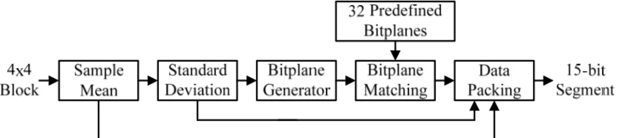
A novel bitplane coding scheme [6] have been proposed based on the conventional BTC. An approaches [7] has been proposed which exploited the visually continuous blocks are encoded as uniform regions, whereas visually discontinuous block are encoded as localized patterns interpreted as edges or lines. Fig. 6 shows the flowchart of Block Truncation Coding using a set of predefined bitplanes. By inverting and rotating, ten basic predefined bitplanes, as shown in Fig. 7, can be extended the 32 predefined bitplanes. In the data packing, the 15-bit bitplane becomes the 6-bit bitplane as shown in Fig. 8.

Although both [6] and [7] based on BTC could reduce the bit number of the bitplane. However, H.264 decoder has the error propagation problem. Thus, in H.264 decoder, they are not suitable for visual quality because their quality loss becomes unacceptable visual quality.

Fig. 6 The compression flow of Block Truncation Coding using a set of predefined bitplanes

Fig. 7 Ten basic bitplanes can be extend the thirty-two bitplanes

Fig. 8 Compressed 16-bit segment format of Block Truncation Coding using a set of predefined bitplanes

2.2.3 Bitplane Truncation Coding

In the beginning, the integer sequence P can be decomposed in binary with a magnitude representation, to form a 8 N× binary matrix, such as (7)

( )

( )

( )

( )

( )

( )

( )

,where is the number of pixels of a block. represents the MSB plane while represents the LSB plane. Then, as shown in

N B₇ B₀

Algorithm 1, the start plane (SP) is

searched for four successive bitplanes from the MSB bitplane. For example, if and are all-0, then SP is equal to 2.

7

B

6

B

Algorithm 1 (Bitplane Truncation Coding Algorithm)

Input: B P( ) is binary matrix.

Output: SP is start plane

( )

( )

( )

if B P is zero vector then SP end if

else if B P is zero vector then SP end else if

else if B P is zero vector then SP end else if

else SP end else return SP

NOT NOT NOT

2.3 Summary

Lossless compression can guarantee no quality loss, but variable length of the compressed data caused irreducible frame memory size. Therefore, existing lossless algorithms are not suitable for frame compression because their primary purpose is high coding efficiency rather than low latency, computation complexity, and high random accessibility. On the contrary, lossy compression algorithm with the fixed CR can guarantee the reduction of frame memory size. Consequently, it is important to design a lossy algorithm with the following features: 1) Low visual quality distortion, 2) Low complexity, 3) Low bandwidth requirement, and 4) Low power consumption.

Chapter 3

Proposed Algorithm

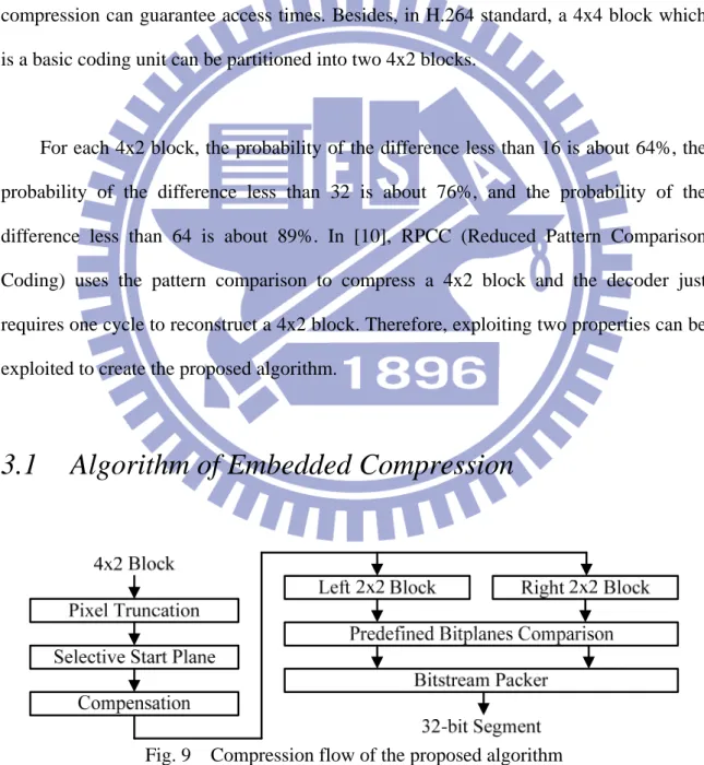
The proposed algorithm compresses a 4x2 block (64-bit) from the output of the deblocking filter. The CR is fixed at 2. After compressing, a 4x2 block will become a 32-bit segment. With fixed CR, the amount of the coded data is constant. Therefore, this compression can guarantee access times. Besides, in H.264 standard, a 4x4 block which is a basic coding unit can be partitioned into two 4x2 blocks.

For each 4x2 block, the probability of the difference less than 16 is about 64%, the probability of the difference less than 32 is about 76%, and the probability of the difference less than 64 is about 89%. In [10], RPCC (Reduced Pattern Comparison Coding) uses the pattern comparison to compress a 4x2 block and the decoder just requires one cycle to reconstruct a 4x2 block. Therefore, exploiting two properties can be exploited to create the proposed algorithm.

3.1 Algorithm of Embedded Compression

Fig. 9 shows the flowchart of the proposed compression algorithm. We divide the algorithm into four parts: 1) Pixel Truncation, 2) Selective Start Plane, 3) Compensation, and 4) Predefined Bitplanes Comparison. These parts will be described in the following paragraphs. The compressed 32-bit segment format is shown in Fig. 10. The representation format consists of 2-bit Mode, 2-bit Start Plane (SP), 2-bit Decision L, 2-bit Decision R, 12-bit Coded Data L, and 12-bit Coded Data R.

Fig. 10 Compressed 32-bit segment format

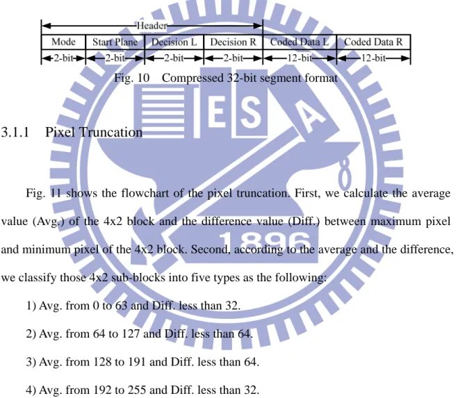
3.1.1 Pixel Truncation

Fig. 11 shows the flowchart of the pixel truncation. First, we calculate the average value (Avg.) of the 4x2 block and the difference value (Diff.) between maximum pixel and minimum pixel of the 4x2 block. Second, according to the average and the difference, we classify those 4x2 sub-blocks into five types as the following:

1) Avg. from 0 to 63 and Diff. less than 32. 2) Avg. from 64 to 127 and Diff. less than 64. 3) Avg. from 128 to 191 and Diff. less than 64. 4) Avg. from 192 to 255 and Diff. less than 32. 5) No change.

In type 1, if each pixel is larger than or equal to 64, we force the pixel to be 63. In type 2, if each pixel is less than 64, we force the pixel to be 64; if each pixel is larger than or equal to 128, we force the pixel to be 127. Types 3 and 4 are processed like types 2 and 1 respectively. In type 5, the original pixel value remains unchanged.

Fig. 11 Flowchart of the pixel truncation

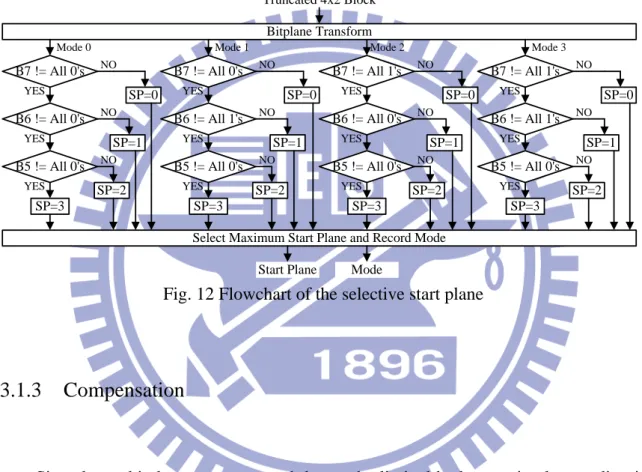
3.1.2 Selective Start Plane

Fig. 14 shows the flowchart of the selective start plane. Bitplane coding is a well-known method. We exploit bitplane as a basic unit to a group numbers, instead of pixel-wised basic unit.

First, we consider a 4x2 block in which each pixel value is represented by 8-bit. A bitplane can be formed by selecting a single bit from the same position in the binary representation of each pixel. We define that B7 represents the MSB plane while B0 represents the LSB plane.

Second, the start plane (SP) is searched for four successive bitplanes from the MSB bitplane with four modes as follows:

1) From B7 to B5 are all-0. 2) B6 is all-1; B7 and B5 are all-0.

3) B7 are all-1; B6 and B5 are all-0. 4) B7 and B6 are all-1; B5 is all-0.

In the first mode, if both B7 and B6 are all-0 and B5 is not all-0, then SP is equal to 1. Similarly, the other modes like as the first mode. Finally, the maximum start plane of four modes is selected to record the mode and start plane.

B7 != All 0's NO YES B6 != All 0's NO YES B5 != All 0's NO YES B7 != All 0's NO YES B6 != All 1's NO YES B5 != All 0's NO YES B7 != All 1's NO YES B6 != All 0's NO YES B5 != All 0's NO YES B7 != All 1's NO YES B6 != All 1's NO YES B5 != All 0's NO YES Bitplane Transform Mode 3 Mode 2 Mode 1 Mode 0 Truncated 4x2 Block

Select Maximum Start Plane and Record Mode SP=0 SP=1 SP=2 SP=3 SP=3 SP=2 SP=1 SP=0 SP=0 SP=1 SP=2 SP=3 SP=0 SP=1 SP=2 SP=3

Start Plane Mode

Fig. 12 Flowchart of the selective start plane

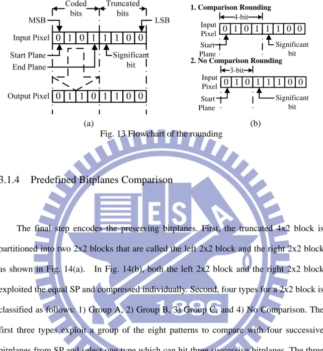
3.1.3 Compensation

Since lower bitplanes are truncated due to the limited budget, a simple rounding is applied here. The rounding is applied when the significant bit of the truncated bits is nonzero and the coded bits are not all 1’s. In Fig. 13(a), the simple idea is shown. This idea leads to a satisfied quality improvement. Two rounding modes are proposed because the pattern comparison has two data compressed formats. As shown in Fig. 13(b), the first one is the comparison rounding and the other is the no comparison rounding. For pattern comparison, the first rounding method is applied to the first three types and the second rounding method is only for the final type.

0 1 0 1 1 1 0 0 Significant bit Start Plane 3-bit Input Pixel 2. No Comparison Rounding 0 1 0 1 1 1 0 0 Significant bit Start Plane 4-bit Input Pixel 1. Comparison Rounding (a) (b)

Fig. 13 Flowchart of the rounding

3.1.4 Predefined Bitplanes Comparison

The final step encodes the preserving bitplanes. First, the truncated 4x2 block is partitioned into two 2x2 blocks that are called the left 2x2 block and the right 2x2 block as shown in Fig. 14(a). In Fig. 14(b), both the left 2x2 block and the right 2x2 block exploited the equal SP and compressed individually. Second, four types for a 2x2 block is classified as follows: 1) Group A, 2) Group B, 3) Group C, and 4) No Comparison. The first three types exploit a group of the eight patterns to compare with four successive bitplanes from SP and select one type which can hit three successive bitplanes. The three groups of the eight patterns are shown in

TABLE 1.If the first three types cannot hit larger than or equal to three bitplanes, the type 4 is chosen and three successive bitplanes from SP are stored.

TABLE 1 Three Group of Eight Predefined Bitplanes

Pattern No. 1 2 3 4 5 6 7 8 Group A 0000 1111 1110 0111 0011 1100 0001 1000 Group B 0000 1111 1110 0111 1010 1001 0110 0101 Group C 0000 1111 1110 0111 1101 1011 0010 0100

(a) (b) Fig. 14 An example of partitioning 4x2 block

3.2 Simulation Results

In the beginning, we first define the formula of MSE (Mean Square Error) and PSNR (Peak Signal to Noise Ratio). The MSE and PSNR are given in (8) and (9),

2 , , 1 1 1 ( W H w h w h w h MSE I P W H = = = × − ×

∑∑

where is the width of the frame, is the height of the frame, is the original frame, and P is the compressed frame.

W H I

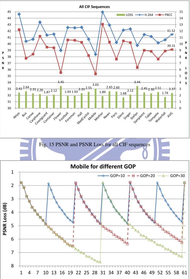
In this section, we focus on the coding efficiency for all CIF sequences. In Fig. 15, PSNR loss is from 1.68 dB to 3.45dB and PSNR loss average is 2.37dB. Then, we show the result of embedded result for different group of picture (GOP) in Fig. 16. Along with the number of P frame, we can see that PSNR loss is growing. Because each P frame is generated by the previous frame which is compressed by our proposed algorithm, the error is bigger and bigger along with the number of P frame. This phenomenon is also called error propagation or drift effect. Fig. 17 shows the results of drift effect with different QP and GOP.

2.41 2.64 2.31 2.20  1.87 2.12  3.45  1.93 1.93 2.33 2.55  3.03  1.89  2.65 2.60  1.68 2.12  3.44  2.45 2.30 2.51  1.74  2.37  41.52  39.15  0  1  2  3  4  5  6  7  8  9  10  11  12  13  14  15  30  31  32  33  34  35  36  37  38  39  40  41  42  43  44  45  P S N R L O S S P S N R All CIF Sequences LOSS H.264 PBCC

Fig. 15 PSNR and PSNR Loss for all CIF sequences

1  2  3  4  5  6  7  8  1 4 7 10 13 16 19 22 25 28 31 34 37 40 43 46 49 52 55 58 61 PSNR  Loss  (dB) Frame

Mobile for different GOP

GOP=10 GOP=20 GOP=30

12.04  8.59  5.72  3.42  13.84  10.24  7.13  4.48  15.04  11.34  8.10  5.24  3  4  5  6  7  8  9  10  11  12  13  14  15  16  20 24 28 32 PSNR  Loss  (dB) QP Value

Mobile for different algorithm

GOP=10 GOP=20 GOP=30

Fig. 17 Drift Effect with different QP and GOP

Chapter 4

Proposed Architecture

In these sections, we will introduce our proposed architecture. In section 4.1, we will describe our proposed embedded compressor. In section 4.2, we will describe our proposed embedded decompressor. In section 4.3, we will show the summary of the proposed architecture and the flow of the design verification.

4.1 Architecture of Compressor

Fig. 18 shows the pipeline architecture of compressor design. We use two pipeline stages and each stage requires one cycle. The first stage is the pixel truncation. The second stage is composed of selective start plane, rounding, selective pattern comparison, and packer. This compressor encodes a 4x2 block in 2 cycles.

Fig. 18 The Pipelined Architecture of Compressor Design

4.1.1 Architecture of Pixel Truncation

Fig. 19 shows the architecture of pixel truncation. There are seven combinational logics, one multiplexer, one de-multiplexer, and one register. The seven combinational

logics as follows: average, difference, type selector, quantizer 1, quantizer 2, quantizer 3, and quantizer 4. The type selector controls the multiplexer and the de-multiplexer. The register stores the truncated 4x2 block.

Fig. 19 Architecture of Pixel Truncation

4.1.2 Architecture of Selective Start Plane

LUT Mode_1 Mode_2 Mode_3 Mode_4 Mode 1 Mode 2 Mode 3 Mode 4 64 64 64 64 64 8

Selective Start Plane

Truncated 4x2 Block 2 2 2 2 Mode Selector 2 2 Start Plane 2 Mode

Fig. 20 Architecture of Selective Start Plane

Fig. 20 shows the architecture of selective bitplane. The block of bitplane transform is a wrapper. There are five combinational logics, one de-multiplexer, and one look-up table. The five combinational logics as follows: Mode 1, Mode 2, Mode 3, Mode 4, and Mode selector. The look-up table records the information of B7 and B6 for each mode.

4.1.3 Architecture of Compensation

Fig. 21 shows the architecture of compensation. There are two combinational logics as follows: Comparison Rounding and No Comparison Rounding.

Comparison Rounding No Comparison Rounding 64

Compensation

Fig. 21 Architecture of Compensation

4.1.4 Architecture of Predefined Bitplanes Comparison

Fig. 22 shows the architecture of pattern comparison. There are five combinational logics, one de-multiplexer, one look-up table and one register. The five combinational logics as follows: Comparison Group A, Comparison Group B, Comparison Group C, and No Comparison. The pattern selector controls the de-multiplexer. The register is stored the coded data.

Comparison Group A Comparison Group B Comparison Group C No Comparison 64 64 64

Predefined Bitplanes Comparison

24 24 24 24 Comparsion Rounding Start Plane 64 No Comparison Rounding LUT 64 2 Selector 24 Coded Data 64 ₄ Regist er 24 Pattern Dicision 4

Fig. 22 Architecture of Predefined Bitplanes Comparison

4.1.5 Data Packing

Fig. 23 shows the architecture of data packing. The representation format consists of 2-bit Mode, 2-bit Start Plane, 2-bit Decision L, 2-bit Decision R, 12-bit Coded Data L, and 12-bit Coded Data R.

Fig. 23 Architecture of Data Packing

4.2 Architecture of Decompressor

Fig. 24 shows the pipeline architecture of decompressor. The decompressor only needs one stage with one cycle. This decompressor reaches a higher throughput; therefore we can provide a higher random accessibility.

Fig. 24 The Pipeline Architecture of Decompressor

4.2.1 Data Rearrange

Fig. 25 shows the architecture of data rearrange. According to the representation format, the data rearrange can be considered as an inverse processing.

Fig. 25 Architecture of Data Rearrange

4.3 Design Implementation and Verification

and the flow of the design verification, respectively.

4.3.1 Design Implementation

TABLE 2 shows the summary of the hardware design. The proposed hardware architecture is synthesized with 90-nm CMOS standard-cell library and the gate count of the proposed algorithm for the compressor and the decompressor are 4.0k and 0.9k, respectively. The working frequency is up to 150MHz@HD1080/720. The proposed embedded compressor is divided into 2 pipelined stages and each stage requires 1 cycle. The proposed embedded decompressor is divided into 1 pipelined stage and each stage requires 1 cycle. For the power consumption, the compressor and the decompressor are 158uW and 86uW@150MHz respectively. As above description, the proposed hardware provides less hardware complexity.

TABLE 2 Summary of the hardware implementation Proposed EC

Function Compressor Decompressor Technology UMC 90nm

Working Frequency HD1080+HD720@150MHz Latency/4x2 block 2 cycles 1 cycle

Gate count 4K 0.9K

Power Consumption 158uW 86uW

4.3.2 Design Verification

Fig. 26 shows the flow of verification. We utilize software and hardware to verify the proposed algorithm. The patterns are created by software and applied as the input of

hardware designs. Then the software calculates the answer to compare with the result of hardware and the result will be stored in memory. Afterward the coded data is accessed by software and hardware decompressor from memory. We check the coded data to confirm the result whether is matched in software and hardware.

Chapter 5

System Integration

In section 5.1, we will introduce Si2 H.264 Decoder System. Then, both access analysis and processing analysis will be discussed in sections 0 and 5.3, respectively.

5.1 System Analysis

Fig. 27 The block diagram of the overall H.264 decoder system

The overall H.264 decoder [3] with the embedded compression codec is shown in Fig. 27. Our H.264 decoder specification is HD1080/HD720@30fps and works at

150MHz. The embedded compressor works between the deblocking filter and the external memory. The embedded decompressor works between the external memory and the motion compensation. To design address controller of EC is very simple since our compression ratio is fixed at two. Our system bus is 32 bits and the external memory is 32 bits per entry.

5.1.1 Interface Problem

Fig. 28 The system interface design for embedded codec

Fig. 28 shows the system; interface design for embedded codec. Between the chip and the off-chip memory, the embedded compression can be considered as an interface. In original H.264 decoder system, here are two interface issues. First interface issue occurs between the deblocking filter and the off-chip memory. The throughput of the deblocking filter is 4 pixels per clock. Therefore, avoiding the pipelined jam at the input of embedded compressor, the processing clocks must be less or equal to 4 cycles. The other issue occurs between the motion compensation (MC) and the off-chip memory. The input of MC requires 4 pixels per cycle, thus the throughput of the embedded decompressor is at least 4 pixels per cycle. Furthermore, since the compression ratio is

fixed at two, the address converter can be easily implemented.

5.1.2 Processing Cycles Problem

In this part, we talk about processing cycle problem of out H.264 decoder system. Our H.264 decoder specification is HD1080/HD720@30fps and works at 150MHz. From our simulation, MC requires average 25 cycles to deal with a 4 4× block. Therefore, embedded compressor requires a fewer-cycle design to reduce the loading cycles.

5.1.3 Overhead Problem

Fig. 29 An example of overhead problem

A block is basic coding unit in H.264 standard. Moreover, due to block-based approaches fit in with block-oriented structure of the received bit-stream, they are most popular techniques. However, here is an overhead problem

4×4

[11] that can be defined as: the ratio between the number of pixels that are actually accessed during the motion compensation of a block and the number of pixels that are really useful in the reference block. In the original system without block-based approaches, the ratio is equal to 1 for

the required pixels accessed. On the contrary, in the original system with block-based approaches, the ratio is always bigger than 1. As shown in Fig. 29, if the required 4×4

block data, we need to fetch four 4×4 block-based data. The overhead in this case is 48.

TABLE 3 Overhead with block grid for six sequences

Sequence 4×4 block grid 8×8 block grid 16 16× block grid

Foreman 1.31 1.77 3.69 Flower 1.30 1.74 3.77 News 1.14 1.51 2.78 Silent 1.17 1.50 3.22 Stefan 1.51 2.44 6.95 Weather 1.17 1.49 3.18 All 1.27 1.73 3.93

As given in TABLE 3, [12] has been provided the summary of the statistical analysis simulated with six sequences. From this table, we can know that the faster motion sequence such as Stefan causes higher overhead. Consequently, it is important that the smaller block-grid can obtain smaller overhead.

5.2 Access Analysis

Fig. 30 shows deblocking filter through the embedded compressor write the data into the external memory and MC through the embedded decompressor read the data from external memory. Moreover, exploiting SystemC, CoWare can build up a simulated platform to analyze the related system problem. As shown in Fig. 31, the user-defined field includes H.264 decoder and EC which is coded in Verilog.

AMBA Slave Interface Embedded Decompressor Motion Compensation Embedded Compressor AMBA AHB External Memory Deblocking Filter H.264 Decoder User-defined CoWare Fig. 31 The Block Diagram of CoWare System

Fig. 32 shows the block diagram of our H.264 decoder with EC in the work space of CoWare platform. The external memory is accepted 128Mb Mobile LPSDR [14] and the bus protocol used AMBA 2.0 with 32-bit bandwidth. After CoWare simulating, we can get the information of the data access as shown in Fig. 33 and Fig. 34.

Fig. 32 Block diagram in CoWare System

Write 4x4 Blocks Read 4x4 Blocks

Fig. 34 Data access trace

5.2.1 Write Reduction

The compression ratio of the proposed EC is fixed at 2. After the proposed EC ( block unit and ) is embedded into our H.264 decoder system, comparing the original system ( block-based access), the reduction ratio of the writing times is 50%.

4×2 CR=2

4×1

5.2.2 Read Reduction

In Motion Compensation, reading required data is based on Motion Vector (MV). Moreover, in MV (x, y), the x value and the y value can be classified as follows:

1) Align: The value is quadruple and the required 4 pixels fits with the block grid. 2) Not Align: The value is not quadruple and an integer. The required 4 pixels traverse two block grids.

4×4

4×4

3) Sub Pixel: The value accurate to 1 / or 1 / . The required 9 pixels can be interpolated into 4 pixels.

2 4

TABLE 4 All Cases of read access required by MC with/without EC

Case of MV (x, y)

Access Cycles for System without

EC

Access Cycles for System with EC Reduction of Access Cycles (%) Probability of Each case (%) (Align, Align) 4 2 50 33

(Align, Not Align) 4 2/3 50/25 0.4

(Align, Sub) 9 5 44.4 5.1

(Not Align, Align) 8 4 50 4.5

(Not Align, Not Align) 8 4/6 50/25 0.4

(Not Align, Sub) 18 10 44.4 5.4

(Sub, Align) 12 6 50 23.5

(Sub, Not Align) 12 6/9 50/25 1.81

(Sub, Sub) 27 15 44.4 25.8

Average 13.2 6.8~6.9 49.1~48.3

In Table II, we analyze the read times of the motion compensation with/without EC. The worst case is the (Sub, Sub) case. To finish the motion compensation, a 4x4 block needs a 9x9 block. Therefore, the system with/without proposed embedded compressor takes 15/27 cycles. The best case is the (Align, Align) case. Original system with/without embedded compressor needs 2/4 cycles to finish the best case. For the other cases when the required data of motion compensation are not fit for 4x2 block-grids, the access times become increased. From our simulation with four sequences (Akiyo, Stefan, Mobile Calendar, Foreman), each 300 frames, we can derive the probabilities of each case. According to the probability of each case, the reduction ratio of the reading times is about 50%.

5.3 Processing Cycle Analysis

In section 5.1.2, the processing cycle problem had been mentioned. In this section, we will talk about the results of our system integration.

Our system specification is HD1080/720@30fps. This specification means each block accepts cycle count in 25 cycles. Because we do not want to change our specification, we wish that MC with the proposed embedded decompressor finishes in 25 cycles. Moreover, based on not to change our specification, we will not to change the data input structure. Here, we must compute the processing cycles as given by

4 4×

MC with Decompressor Decompressor MC without Decompressor

Proccesing Time = Delay +Proccesing Time (10) TABLE 5 shows the processing cycle analysis for all cases. Excluding the (Sub, Sub) case, each case is less than 25 cycles. The average of processing cycles for MC without EC is 17.4 cycles. Therefore, the proposed embedded compression can be embedded into our H.264 decoder system.

TABLE 5 All Cases of Processing Cycle Analysis for EC

Case of MV (x, y) Number of Blocks Delay for our EC Decoder Processing Cycles for MC with our EC Processing Cycles for MC without EC Prob. of Each case (%) (Align, Align) 1 2 4 6 33 (Align, Not Align) 2 2 4 6 0.4

(Align, Sub) 3 3 9 12 5.1 (Not Align, Align) 2 3 8 11 4.5 (Not Align, Not Align) 4 4 8 12 0.4 (Not Align, Sub) 6 6 18 24 5.4 (Sub, Align) 3 3 12 15 23.5 (Sub, Not Align) 6 6 12 18 1.81 (Sub, Sub) 9 8 27 35 25.8

Average 4.1 4.2 13.2 17.4

5.3.1 Access Reduction Ratio

The access ratio of the system with/without EC is given in (11)

System with EC System with EC

System without EC System without EC

Read +Write Access Ratio =

Read +Write (11)

From the simulation, the ratio of read times with/without EC is 0.517, the ratio of write times with/without EC is 0.5, and the average access ratio of read/write in the system without EC is about 3.51. The overall access ratio is given in (12)

0.517 3.51+0.5 1 Overall Access Ratio =

3.51 1 = 51.3%

× ×

+ (12)

The average reduction ratio on memory accessed is given in (13)

(13) Average Reduction Ratio = 1 - Overall Access Ratio

= 1 - 0.513 = 48.7% Therefore, the average reduction ratio is 48.7%.

5.3.2 Simulation Result on Power Reduction

We exploit the system-power calculator [13] as a external memory power model and set the parameter as [14]. The simulation of memory is employed on HD1080/720@150MHz. The simulation results are shown in Fig. 35. Including the core power of H.264 decoder, SDRAM background power and SDRAM access power (read/write).

0 50 100 150 200 250 Power_Original_System Power_EC_System mW Power_EC Power_SDRAM

Fig. 35 Power analysis on HD1080/720@150MHz

Chapter 6

Conclusion and Future Works

6.1 Conclusion

In this thesis, we have proposed a new embedded compression algorithm for mobile video applications. With these advantages of the proposed EC algorithm, we can lessen the size of external memory and bandwidth utilization to achieve power saving. The pipelined architecture of the proposed decompressor requires 1 cycle, thus the random accessibility becomes better. Due to the fixed CR, the proposed EC algorithm is easier to be integrated with H.264 decoder.

From the experimental results, the PSNR loss of the proposed EC algorithm is from 1.89 to 3.45dB. The proposed architecture is synthesized with 90-nm CMOS standard-cell library and the gate counts of the proposed algorithm for compressor/decompressor are 4.0k/0.9k respectively. The working frequency is up to 150MHz@HD1080/720. For power consumption, the compressor is 158uW and the decompressor is 86uW.

6.2 Future Work

For the lossy embedded compression, reducing the visual quality distortion, it is the major objective. From our experimental results, error propagation is worth to be improved. For the simulation results of all I frames, between the original sequence and the compressed sequence, the differences are hardly found. However, for 1I/29P frames,

the drift effect can be found easily in the simulation results. Therefore, we can refine the proposed lossy embedded compression algorithm, such as adaptive predefined bitplanes, additive lossless embedded compression algorithm, and et al, to get better coding-efficiency.

Bibliography

[1] “Draft ITU-T recommendation and final draft international standard of Joint Video Specification (ITU-T Rec. H264-ISO/IEC 14496-10:2005 AVC),” JVT G050, 2005. [2] T. Wiegand, G. J. Sullivan, G. Bjontegaard, A. Luthra, “Overview of the

H.264/AVC video coding standard,” IEEE Trans. Circuits Syst. Video Technol., vol. 13, no. 7, pp. 560-576, Jul. 2003.

[3] T. M. Liu, and et al., “A 125/spl mu/w, fully scalable MPEG-2 and H.264/AVC video decoder for mobile applications,” in Proc. IEEE Int. Solid-State Circuits Conf.

(ISSCC), pp. 1576-1585, 2006.

[4] J. Kim, and C. M. Kyung, “A Lossless Embedded Compression Using Significant Bit Truncation for HD Video Coding,” IEEE Trans. Circuits Syst. Video Technol., early access, 2010.

[5] E.J. Delp, O.R. Mitchell, “Image compression using block truncation coding,” IEEE

Trans. Comm., vol. 27, issue 7, pp. 1335-1342, Sep. 1979.

[6] C. K. Yang and W. H. Tsai, “Improving block truncation coding by line and edge information and adaptive bit plane selection for gray-scale image compression,”

Pattern Recognition Letter, vol. 16, pp. 67-75, 1995.

[7] T. M. Amarunnishad, V. K. Govindan, and T. M. Abraham, “Block Truncation Coding Using a Set of Predefined Bit Planes,” in Proc. IEEE Int. Conf.

Computational Intelligence and Multimedia Applications (ICCIMA), vol. 3, pp.

73-78, Dec. 2007.

[8] T. Y. Lee, “A New Frame-Recompression Algorithm and its Hardware Design for MPEG-2 Video Decoders,” IEEE Trans. Circuits Syst. Video Technol., vol. 13, no.6, pp. 529-534, Jun. 2003.

[9] Y. D. Wu, Y. Li, and C. Y. Lee, “A Novel Embedded Bandwidth-Aware Frame Compressor for Mobile Video Applications,” in Proc. IEEE Intelligent Signal

[10] C. C. Yang, “An Embedded Codec based on Reduced Pattern Comparison Coding for Mobile Devices,” Master’s thesis, National Chiao Tung University, Jan. 2010. [11] Y. D. Wu, “Design of An Embedded Compressor/Decompressor for Mobile Video

Application,” Master’s thesis, National Chiao Tung University, Sep. 2009.

[12] A. Bourge and J. Jung, “Low-Power H.264 Video Decoder with Graceful Degradation,” in SPIE Proc. Visual Comm. And Image Processing, vol. 5308, pp. 372-383, Jan. 2004.

[13] Micron® Technology Inc. The Micron® System-Power Calculator: SDRAM. [Website]:http://www.micron.com/support/part_info/powercalc

[14] Micron® Technology Inc. MT48H4M32LFB5-6 128Mb Mobile LPSDR. [Website]:http://www.micron.com/products/partdetail?part=MT48H4M32LFB5-6

作 者 簡 歷

姓名

：林建辰

戶籍地 ：台灣省彰化市

出生日期：1980 年 8 月 9 日

學歷：

1995 年 9 月~ 2000 年 6 月 國立雲林工專 電機科

2000 年 9 月~ 2002 年 6 月 大華科技大學 電機工程系

2005 年 2 月~ 2009 年 6 月 國立交通大學 IC 設計產業研發碩士專班