The igneous provinciality in Taiwan: Consequence of continental rifting superimposed by Luzon and Ryukyu subduction systems

(1)

NI! ;i

E L S E V I E R Fuzzy Sets and Systems 101 (1999) 343-352

F U | | Y

sets and systems

Fuzzy system identification using an adaptive learning rule

with terminal attractors

Chuan-Kai Lin, Sheng-De Wang*

Department of Electrical Engineerin 9, EE Buildin 9, Rm. 441, National Taiwan University, Taipei 106, Taiwan

Received December 1995; received in revised form March 1997

Abstract

A fuzzy model with an adaptive learning rule is proposed to approximate a class of nonlinear systems. The proposed adaptive learning rule uses the concept of terminal attractors and guarantees that the identification is stable and fast convergence in finite time. Another subject of this paper is to determine the appropriate rule number of the fuzzy model required for a desired modeling error. A learning algorithm is also introduced to identify the centers of membership fimctions of fuzzy outputs. @ 1999 Elsevier Science B.V. All rights reserved.

Keywords." Fuzzy model; Terminal attractor; Adaptive learning rule; System identification

1. Introduction

The mathematical models of complex and nonlinear systems are often very difficult to obtain. However, control engineers always face the problems of control- ling and modeling such systems. In recent years, there has been growing interest in using neural networks and fuzzy set theory for modeling nonlinear and complex systems because fuzzy models offer a framework for combining linguistic information and numerical data in a unified fashion. However, most tasks are dedicated to tuning parameters of fuzzy models [14, 11]. As for the topic of determining the rule number, it is still worth for researching a systematic approach.

When designing a fuzzy model, we shall first determine the number of rules and the modeling accuracy.

* Corresponding author.

Then, use a learning algorithm to find out the free parameters of the model. The determination of an appropriate number of rules is not an easy task since it is a nontrivial function of modeling accuracy. In previous research work [14], the number of rules is, in general, given a priori by experienced designers. Therefore, we present a systematic method to determine the number of rules.

This paper is written with two main objectives. The first is to introduce a method for determining the number of rules of fuzzy model. The second objective is to develop a fast on-line learning rule to adjust free parameters of the proposed model. The concept of terminal attractors [18], which has fast convergence property, is incorporated into the adaptive learning rule. Hence, the adaptive learning rule provides properties of stability and convergence in finite time. The convergence rate of our approach is faster than conventional system identification with the backprop- agation algorithm.

(2)

344 C-K. Lin, S.-D. Wang/Fuzzy Sets and Systems 101 (1999) 343-352 A fuzzy model or a fuzzy logic system, can be

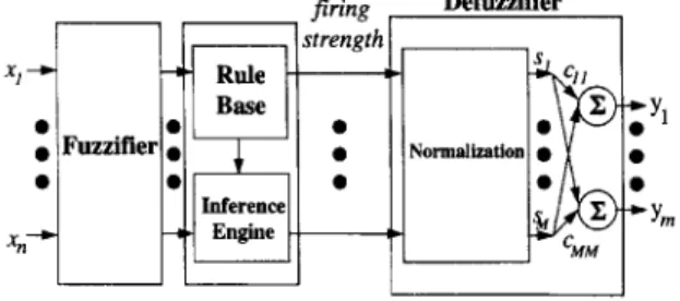
composed of four components: a fuzzifier, a fuzzy rule base, a fuzzy inference engine and a defuzzifier. The detailed description of the four components can be found in [5, 6]. Therefore, we just review them briefly.

Consider a fuzzy system:

U C R'---~ R m,

where U is a compact set of universe discourse and n is the dimension of the input space and m is the dimension of the output space. The purpose of the fuzzifier is to map the real inputs to the fuzzy sets, which are charac- terized by membership functions #F : U ~ [0, 1] and represent linguistic terms such as "small", "medium" and "large". The shape of membership functions may be triangular, trapezoidal and Gaussian-like functions.

After the fuzzification process, we enter the fuzzy inference engine that employs fuzzy rules to map from fuzzy sets in input space to the fuzzy sets in output space. Assume that there are M rules in the fuzzy rule base and all are in the following form:

IF xl is ,4jl and

x2

is Aj2 a n d . . , and x~ is ,4j, THEN Yl is/}lj and ... and

Ym

is

Bmj.

In the above rules, xi are the real inputs into the fuzzy system, Yk are the output variables of the fuzzy system and

,4ji

and/~kj are linguistic terms character- ized by membership functions #A)

(Xi)

and

pg~j (Yk),

respectively. By using fuzzy logic operations such as T-norm, the fuzzy inference engine determines the fuzzy outputs. The last procedure is to find a corresponding value in the problem domain using a defuzzi- tier that usually employs the center-of-area method. In this paper, a form of center-average defuzzifica- tion and the singleton fuzzification will be used in the proposed fuzzy model.

The paper is organized as follows. In Section 2, we will introduce the architecture of a fuzzy model and discuss the methodology to construct the fuzzy model. In Section 3, we construct the nonlinear identifiers with an adaptive learning rule for continuous systems. The stability and convergence of estimated errors are also analyzed in this section. A design algorithm sum- marizes the approach proposed in Sections 2 and 3. Section 4 then shows the simulation results. At last, Section 5 concludes the paper.

2. The proposed fuzzy modeling approach

The fuzzy logic systems with a center-average defuzzifier and a singleton fuzzifier can be represented as linear combinations of functions of normalized firing strength. From the kth output of the center-average defuzzifier, )3 k, is as follows:

k(x) = )5;_-'", N"

_{i=l #X,,(xi)}

₍₁₎

k = l , 2 . . . m,

where ~kj's are the centers of fuzzy outputs. Here )3 k can be viewed as the linear combination of normalized firing strength

qgj(x)

which is defined as follows. Definition 1

(Normalized firing strength).

Define the normalized firing strength as

flJ

(2)

flj= [ ]pAi,(xi),

j = 1,2 . . . M, (3) i=1

where

#~j,(xi)

are membership functions, M is the rule number, ["] is the implication operator and

From the above description, we can view the defuzzifier as a summation of products of the normalized firing strengths and centers. As a result, the fuzzy model f can be represented in the following form:

f = a/Ys

(4)

and

y(t)

= f ( x ) = f ( x ) +

e(t),

(5)

where y : [Yl y2 ...

Ym] T, e(t)

is the model error vector, s = [Sl s2 ... SM] T is the firing strength and IT" is an

M×m

real adjustable parameters matrix with entry ffkj. The fuzzy model is shown in Fig. 1. For the single-output case, we assume

f ( x )

is continuously differentiable ( q + 1 ) times and the ( q + 1 )th derivative of

f ( x )

is also bounded, i.e., 1[~7q+lf(x)[[2 <

m t

for all x E U ([1 - [1 is the induced norm). For the case of the Gaussian membership function, we can use a

(3)

C.-K. Lin, S.-D. Wang~Fuzzy Sets and Systems 101 (1999) 343-352 345 firing Rule strength: xl -~• Base • • • Fuzzifier Inference~ I •• Xn-~ Engine : Defuzzifier

hi-

~Yl ~y~

is within the specified upper error bound. The ~-cut fuzzy set is incorporated into the modified method. The set of elements that belong to the fuzzy set .4 at least to the degree ct is called the or-level fuzzy set or e-cut fuzzy set:

= {x c u I

Fig. 1. The structure of fuzzy model. Hence, we define a modified firing strength function _as

center vector

ej

to represent the n input centers of the jth rule. In [3], an inequality is obtained by Taylor's

expansion to guarantee the existence of f ( x ) :

M

< o,

j=l

(6)

where

9j(x) = Ilx -

cjll q+l

-

e(q + 1)[/Mf

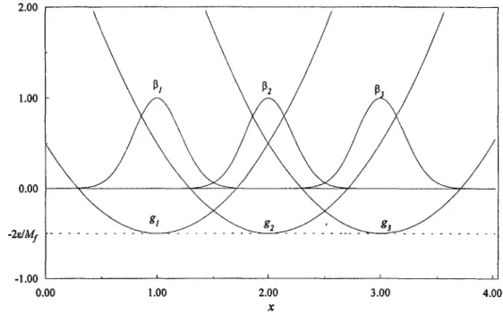
and e is an arbitrary real number. If inequality (6) holds for all x E U, then I I f ( x ) - f ( x ) l l 2 <e. A geometric interpretation is illustrated in Fig. 2.

Johansen and Foss used inequality (6) to construct a global nonlinear ARMAX (NARMAX) model by interpolating local ARMAX models that are valid within certain operating regimes [3]. The local model validity functions are defined to indicate the relative validity of local models at a given operating point. Each local model validity function,

flj(x),

which is a Gaussian function, is defined to indicate the relative validity of the corresponding local model at a given operating point. The local model validity function bears analogy to the firing strength; the operating regime has analogy to the rule which has strongest firing strength. However, we can find out the differences between NARMAX models and fuzzy models. Johansen and Foss suggested that the width of the local model validity functions go to zero for satisfying inequality (6). From the point of view of fuzzy systems, it means that there is only one rule to be fired at each state. This phenomenon distinguishes the NARMAX model from the fuzzy model since fuzzy systems always fire several rules as a result of fuzzy reasoning. Hence, we can modify the method proposed by Johansen and Foss for fuzzy systems to determine the rule number of fuzzy rule base such that the modeling error

/~= {0, /~j<~,

(7)

In Fig. 3, it is obvious that the width of

flj(x)

is not necessarily small enough to satisfy inequality (6) after applying the e-cut fuzzy set. We also propose a modified firing strength function which is capable of enlarging the width and can be incorporated into the adaptive learning rule as will be discussed in Section 3. Definition 2

(Modified normalized firing strength

function).

Define the modified normalized firing

strength function sj as

sj(x)=

II/vll2' j = 1,2 . . . M (8)

M :t 2

where/V= [fl]' fl~.., fl~t] x and II/V 112 = V/~j=I (flj) • And the normalized firing strength function has the property }-~M_, 4 = 1.

As

MU

and e are given, the shapes ofgj-functions are determined. The location of a g j-function is associated with the flj and it is free to choose :t and flj such that inequality (6) holds. However, the rule number M must be sufficiently large to cover the whole input space of interest. The basic idea of designing premises of fuzzy rules is to cover all input space by satisfying inequality (6). Take a simple example to illustrate the above discussion. Assume

f ( x ) = x +

sin(x/2), q is chosen as 1 and the accuracy ~ is set to be 0.01, and the gj-functions are given by

gj(x)

=

IIx - cjll~

- 0.08

(Mr

= 0.25). For covering the interval [0.0, 2n], there are 11 rules with ~ = 0.3 as shown in Fig. 3. The boundary of the operating region of each rule is determined by the e-cut fuzzy set.

(4)

346 C-K. Lin, S.-D. Wang~Fuzzy Sets and Systems 101 (1999) 343 352 2.00 c6." 1.00 0.00 -2e./~l,ff -1.00 0.00 1.00 2.00 3.00 4.00 x

Fig. 2. Geometrical interpretation of Johansen and Foss method.

membership functions and gj

1.00

ct=0.4

0.00 -2~/Mf =-0.08

Art A21 A31 A41

?472 7482

A91 A]o I !111

Q glo gr

I I I I

0.00 2.00 4.00

Fig. 3. Geometrical interpretation of Eq. (6): f ( x ) = x + sin(x/2).

(5)

C.-K. Lin, S.-D. Wang/Fuzzy Sets and Systems lO1 (1999) 343-352 347

3. Adaptive learning rule with terminal attractors the jth rule to the kth output. Hence, In the previous section, the method of construct-

ing the premise structure (IF parts) of a fuzzy model has been developed and there remain free parameters in the consequent structure (THEN parts) to be identified by adaptive learning rule which will be discussed in this section. The proposed adaptive learning rule makes use of the concepts of terminal attractors and has the fast convergence rate and stability properties. On the other hand, there is a trade-off between the fuzzy rule number and the modeling error bound• The smaller the error bound is, the more the fuzzy rules will be obtained. Thus, we prefer to use a some- what larger error bound to make the rule base small. Therefore, a robust adaptive technique [9-11 ] is added to reduce the approximating error. As a result, the specified upper error norm is not required to be very small to obtain the required approximation accuracy.

In this paper, we are concerned with the model identification of single-output-multi-input systems. The multi-input and multi-output fuzzy model can be di- vided into multi-input and single-output groups. It has been proven that if the mapping is well-defined then the fuzzy model is capable of approximating any real continuous function to arbitrary accuracy [ 14]. There- fore, we make the following assumption.

Assumption 1. There exists a coefficient vector matrix w; such that the optimal fuzzy model f * approxi- mates the continuous function f , with accuracy e over a compact set U, that is, 5W~ such that

M

yk(t) - f~k(t) = E rbki(t)sj(x) + gk = ek,

j : l

(11)

where wkj = w~j - ~k~ and gk = ek - gk. As the number of rules is fixed, the smallest achievable ek can be determined. The modeling problem can thus be solved if we can use an adaptive learning law for tuning ff~kj and driving the errors ek to zero. The weights of the kth output of the fuzzy model and the estimated error can be continuously, respectively, updated as

v~kj=qlkePsj(x), 0 < p < l (12)

and

~k = rl2ke p, (13)

where ~lk and/~2k are positive constants determining the adaptation rates. Eqs. (12) and (13) constitute the adaptive learning rule. The introduction of estimated errors in (13) makes the equilibrium points of dynamic equations (12) and (13 ) become terminal attractors [8] that can guarantee the stability and convergence to the arbitrary small neighborhood of zero in finite time. Define the squared error E = ½e2(t)=

½(Yk(t) - )32(t)) 2 as the error measure for the identification task. Now, a stability theorem is presented for the adaptive learning rule.

m a x l f ( x ) _{- f} * x ₍

_{,WT)I~<~, vx~u.}

According to the above assumption, there exists w]

and ek such that the actual yk(t) is given by

M

yk(t) = E wk*/(t)sj(x) + ek,

j = l

(9)

Theorem 1. Applying the adaptive learning rule (12)

and ( 13)for f u z z y model (10). We have the Jbllowing properties.

(a) Output error ek = 0 is a terminal attractor o f the dynamic equation describin 9 E and

(b) the estimated parameters ff~kj o f the fuzz), model will remain bounded.

and the estimated output )Sk(t ) is given by M

Yk(t) = E ~kj(t)s/(x) + gk,

/=1

(10)

where ff~ki's are an approximation to the optimum centers of membership functions in THEN parts from

Proof. (a) For proving that ek = 0 is a terminal attractor, compute the time derivative of E as follows:

(6)

348 C-K. Lin, S.-D. Wang~Fuzzy Sets and Systems 101 (1999) 343-352

)

- r h k k s ) ( x ) - ~12ke~ j = l l+p = - rle k = - qE 7, (15)

where q = 2(l+P)/2(qlk q- q2k) is a positive constant and 0 < 7 = ( 1 + p ) / 2 < l . For E(0)>~0, the above equation implies that /~ ~< 0 with terminal attractor E = 0 , i.e. ei=O.

(b) Consider the Lyapunov function candidate:

Step 3: For j = 1 to M

& = A u~,, (xi).

i=1

Step 4: For j = 1 to M do Steps 5-6. Step 5: Calculate sj.

Step 6: For k = 1 to m do Steps 7-8. Step 7: Calculate kth output error ek. Step 8: ffkj =

rhkefsj(x)

and ,~,~ = r/ekeff.

1 M

_{Wk j q_}

5J_

_g2.

j = l q2k

(16)

Using Eqs. (12) and (13), we have

1 J I p + - - g k ( - q2ke k ) rl2k = - ~I E~. (17)

Thus, we have /2 ~ < - r/E~' for all t 1>0, and for E/> 0, V will be asymptotically converged. Therefore, we can conclude that if #kj are bounded at time t = 0, they will remain bounded for all t > 0. []

From Sections 2 and 3, we can conclude an algorithm to design the fuzzy model for identifying the given system.

4. Simulation

There are two examples in this section. The first is the prediction of chaotic time series, and the second is to identify a multi-input and multi-output model. The plant dynamics were simulated in C language with Runge-Kutta algorithm on a Pentium 75 MHz PC. Example 1. In this example, the fuzzy model is used to predict chaotic time series [10]. Chaotic time series, which can be generated by deterministic method, are complicated as random time series. The following discrete equation can generate chaotic time series:

y[k] = 7 y [ k - 1](1 - y [ k - 1]),

where the chaotic behavior appears for certain choices of 7, for example, 7 = 3.75. Fig. 4 shows a part of the chaotic series that are used in the simulation.

In the simulation, the rulebase with 225 rules has the following form:

Design Algorithm

Input: 1. Given a desired modeling error e and My,

that is the upper bound of first order derivative of the vector function f over x.

2. Number of data patterns for identification: N. 3. Data patterns for identification and output dimension m.

Output: Rule number M and coefficient wkj ( j =

1 . . . . ,M, k = 1 . . . m).

Step 1: Determine M by Eq. (6). Step 2: For l = 1 to N do Steps 3-8.

IFy[k - 1] is 41 and y[k - 2] is Ajz

THEN y[k] i s / ~ j l , j = 1,2,..., 225.

Each input variable is assigned to 15 membership functions for satisfying (6) and 9 j ( x ) =

IIx - cjll~

-

e ( 2 / M f ) (e = 0.005 and My = 7.5). The Gaussian-like

membership functions are # d j , ( x i ) = e x p ( - 6 O O ( x i - cji) 2) where cji = 0.2 + 0.6(j - 1 ). Therefore, the fir-

ing strength/~j = exp{-600[(xl - cjl )2 + (x2 - cj2)2]}

and c~ and */lk (=r/2k) are set to 0.3 and 0.02, respectively. This simulation took about 40s on a Pentium-75 MHz PC with 16 MB RAM. The recent proposed approach in [14] is a similar model with a

(7)

1.20

C-K. Lin, S.-D. Wang/Fuzzy Sets and Systems 101 (1999) 343-352

Chaotic time series

349 0.80 0.40 0.00 9500 9550 9600 9650 9700 9750 9800 9850 9900 9950 k

Fig. 4. The chaotic time series y[k] = c~y[k- 1](1 - y [ k - 1]) from k = 9500 to 10000 (a = 3.75).

I0000 1.00 predicted error 0.50 0.00 -0.50 0 1000 2000 3.000 4000 5000 6000 7000 8000 9000 k

Fig. 5. The predicted error of the chaotic time series y[k] = cry [ k - 1](1 - y [ k - 1]) (ct = 3.75).

(8)

350 C.-K. Lin, S.-D. Wang~Fuzzy Sets and Systems 101 (1999) 343-352

2.00

Predicted Error (MIMO)

e,i

0.00

-2.00

-4.00

-6.00 Ypl : desired trajectory

. . . ~plt : trajectory(with terminal attractors) after 200 time steps . . . .~#2 : trajectory(with neural networks) aRer 100000 time steps

-8.00 4.00 0.00 2.00 1.00 0.00 -1.00 -2.00 -3.00 -4.00 10.00 20.00 30.00 40.00 50.00 60.00 70.00 80.00 90.00 T i m e Step k

(a)

Predicted Error (MIMO)

Yp2 : desired trajectory

. . . .9p21 : trajectory(with terminal attractors) attar 200 time steps . . . .~p22 : trajectory(with nepal networks) after 100000 time steps

100.00

i

0.00 10.00 20.00 30.00 40.00 50.00 60.00 70.00 80.00 90.00 T i m e Step k

(b)

Fig. 6. MIMO model identification for (a) ypl[k], (b) Yp2[k].

(9)

C.-K. Lin, S.-D. Wang/Fuzzy Sets and Systems 101 (1999) 343-352 351

different learning algorithm which needs to compute an inverse matrix. Another approach is Gaussian neural networks. The architecture of Gaussian neural networks is too large (a total of 5776 nodes [10]) and it cannot represent the knowledge of linguistic rules. The approach proposed in this paper can complement the drawbacks.

The predicted error

e(t)

is defined as the difference between the chaotic time series

y[k]

and the estimated time series ~(t), i.e. e ( t ) = J?(t) -

x(t).

The upper error bound is set to 0.005. Fig. 5 shows most of the predicted error fall into the error bound as expected.

achieves two objectives successfully: one is to determine the appropriate size of the fuzzy rulebase and another is to propose a new adaptive rule to learn the centers of output fuzzy sets. The first step of designing a fuzzy rulebase is to determine the rule number by the method described in this paper. As the number of rules and the linguistic IF part has been determined, the THEN part can be on-line tuned by the adaptive learning rule while the learning algorithm in [14] is off-line. Due to the introducing of terminal attractors, the convergence rate is very fast. Therefore, the meth- ods proposed in this paper are effective.

Example 2. In this example, it is shown that the MIMO plants can be identified by a MIMO fuzzy model which is composed of several multi-input and single-output groups. A nonlinear two-input and two-output plant is described as the following equations [7]:

ypl [k]

y p , [ k + 1]1 I + y p 22[k] [ Ul[k] ]

yp2[k 4- 1] : -

ypl[k]yp2[k]

+ /u2[k]J '

1 + y 2Ek]

where Ul[k] and

u2[k]

are inputs and

ypl[k]

and

yp2[k]

are outputs. In the simulation, [ul[k] uz[k]] v = [sin(27zk/25) cos(27tk/25)] T and the resultant fuzzy rulebase has 81 rules. Since there are four fuzzy variables

ypi

[k],

ypz[k], Ul

[k] and ue[k] are in the IF part and each fuzzy variable has three linguistic terms. The rulebase can be interpreted in the following forms: IF

Ypl[k]

is P and

yp2[k]

is Z and Ul[k] is N and uz[k] is P then

ypl[k +

1] is Z and

ypz[k +

1] is Z.

The simulation results are shown in Fig. 6. The neural network proposed in [7] using 100000 time steps to identify the system; however, our method only needs 200 time steps to achieve acceptable results. This implies the proposed model can identify a nonlinear MIMO dynamic system and has the fast convergence rate.

5. Conclusion

In this paper, we have considered the problem of system identification using neural fuzzy models and

References

[1] J.J. Buckley, Numerical relationships between neural networks, continuous functions, and fuzzy systems, Fuzzy Sets and Systems 60 (1993) 1-8.

[2] J.J. Buckley, Y. Hayashi, Hybrid neural nets can be fuzzy controllers and fuzzy expert systems, Fuzzy Sets and Systems 60 (1993) 135-142.

[3] T.A. Johansen, B.A. Foss, Constructing NARMAX models using ARMAX models, Internat. J. Control 58 (1993)

1125-1153.

[4] J.M. Keller, R.R. Yager, H. Tahani, Neural network implementation of fuzzy logic, Fuzzy Sets and Systems 45 (1992) 1-12.

[5] C.C. Lee, Fuzzy logic in control systems: Fuzzy logic controller, part I, IEEE Trans. Systems Man Cybernet. 20 (1990) 404-418.

[6] C.C. Lee, Fuzzy logic in control systems: Fuzzy logic controller, part II, IEEE Trans. Systems Man Cybernet. 20 (1990) 419-435.

[7] K.S. Narendra, K.P. Parthasarathy, Identification and control of dynamic systems using neural networks, IEEE Trans. Neural Networks 1 (1990) 4-27.

[8] W. Pedrycz, Fuzzy neural networks and neurocomputations, Fuzzy Sets and Systems 56 (1993) 1-28.

[9] R.M. Sanner, J.-J.E. Slotine, Gaussian networks for direct adaptive control, IEEE Trans. Neural Networks 3 (1992) 837 863.

[10] R.M. Sanner, J.-J.E. Slotine, Stable recursive identification using radial basis function networks, in: Proc. American Control Conf., 1992, 1829-1833.

[11] C.-Y. Su, Y. Stepanenko, Adaptive control of a class of nonlinear systems with fuzzy logic, 1EEE Trans. Fuzzy Systems 2 (1994) 285-294.

[12] M. Sugeno, K. Tanaka, Successive identification of a fuzzy model and its application to prediction of a complex system, IEEE Trans. Systems Man Cybemet. 42 (1991) 315-334. [13] T. Takagi, M. Sugeno, Fuzzy identification of systems and its

applications to modeling and control, IEEE Trans. Systems Man Cybemet. 15 (1985) 116-132.

(10)

352 C-K. Lin, S.-D. Wang/Fuzzy Sets and Systems 101 (1999) 343-352

[14] L.X. Wang, J.M. Mendel, Fuzzy basis functions, universal approximation, and orthogonal least-squares learning, IEEE Trans. Neural Networks 3 (1992) 807-814.

[15] L.X. Wang, J.M. Mendel, Generating fuzzy rules by learning from examples, IEEE Trans. Systems Man Cybernet. 22 (1992) 1414-1427.

[16] C. Xu, Y. Lu, Fuzzy model identification and self learning for dynamic systems, IEEE Trans. Systems Man Cybemet. 17 (1987) 683-689.

[17] S. Yeong, M.J. Chung, Identification of fuzzy relational model and its application to control, Fuzzy Sets and Systems 59 (1993) 25-33.

[18] M. Zak, Terminal attractors in neural networks, Neural Networks 2 (1989) 259-274.