國 立 交 通 大 學
交通運輸研究所
博 士 論 文
No.064
汽機車混合車流模擬
—新細胞自動機模
型之研發
Car/Motorcycle Mixed Traffic Modeling: A New
Cellular Automaton Approach
指導教授:藍武王博士、邱裕鈞博士
研 究 生:林日新
汽機車混合車流模擬
—新細胞自動機模型之研發
Car/Motorcycle Mixed Traffic Modeling: A New Cellular
Automaton Approach
研 究 生:林日新 Student: Zih-Shin Lin
指導教授:藍武王博士 Advisors: Dr. Lawrence W. Lan
邱裕鈞博士 Dr. Yu-Chiun Chiou
國 立 交 通 大 學 交 通 運 輸 研 究 所
博 士 論 文
A Dissertation
Submitted to Institute of Traffic and Transportation
College of Management National Chiao Tung University in Partial Fulfillment of the Requirements
for the Degree of Doctor of Philosophy in
Management
June 2010
Taipei, Taiwan, Republic of China
汽機車混合車流模擬
-新細胞自動機模型之研發
研 究 生:林日新 指導教授:藍武王博士、邱裕鈞博士國立交通大學交通運輸研究所
摘要 細胞自動機模型可分類為一種微觀的數值模擬車流模型,近年來世 界各地學者曾提出多種不同的細胞自動機車流模型,用以模擬現實生活中 各種複雜的交通現象。但由於目前細胞自動機模型主要應用相對稀疏之格 點系統,導致其無法應用於都市之交通模擬,因此本研究提出一種全新的 細胞自動機模型,以克服上述限制,並將細胞自動機模型之應用範圍擴展 至都市交通之模擬。 本研究基本上可分為三部份,首先,本研究提出一個具細微格點系 統之細胞自動機模型,以提昇進行交通模擬時之模型解析度,並有效反應 微觀的交通車流特性。與現有其它細胞自動機車流模型相較,本研究所提 出細微格點系統之細胞自動機模型主要有三項明顯差異;首先本研究提出 「共有單元」的概念做為描述不同車輛尺寸及不同道路寬度的共同基本單 元,而一單獨細胞單位及網格則分別定義為車輛及道路之基本單元。其次 本研究提出立體通用交通參數之觀念,如此於進行交通模擬時可將不同車 輛尺寸及不同道路寬度之影響納入評估。以上述細微格點系統之細胞自動 機模型為基礎,本研究並建議採用線段線性變化之車輛速度變化方式,接 下來本研究並將車輛之減速能力亦納入交通模擬之分析範圍,以改正現有 多數細胞自動機模型模擬結果中普遍存在的一個重要瑕疵,亦即當車輛遭 遇障礙物或抵達塞車車陣之後緣時會有不合理的急速刹車行為。本研究所 構思的減速機制事實上源起於1950 年代美國學者 Pipes 及 Forbes 等人所提 出原始車流理論。後續模擬結果證實,本研究所提出之減速機制已成功改 正現有細胞自動機模型上述車輛不合理減速現象。 其次,本研究建立於應用上述細微格點系統之細胞自動機模型進行 交通模擬時擷取區域路段交通參數數據之有效方法。模擬結果亦證實透過上述方式所擷取之區域路段交通參數資料除可成功印證德國知名學者 Kerner 於 2004 年所提出之三相車流理論外,並可描述三種車流車相間之 相變化。 在本研究的第三部份中,藉由上述改良之細微格點系統,對由汽車 及機車所組成之混合車流形態之交通特性進行模擬及分析。模擬結果證 實,本研究所提出之細胞自動機模型可模擬一些重要的都市交通之混合車 流現象,如機車於塞車車陣中之橫向移動或由車陣後方兩輛並排車輛間空 隙鑽入車陣之複雜行為。 雖然現有之細胞自動機車流模型仍廣受認同,但仍持續有人質疑其 應用範圍多限縮於高速公路交通模擬,且無法由微觀角度成功描述細微之 車輛行為。反之,透過模擬結果分析,可印證本研究所提出新細胞自動機 模型之優越性,因其成功地克服一般現有細胞自動機車流模型之適用限 制,將可用以分析實際生活中多變的交通現象。基於本研究所提出新細胞 自動機模型具有高解析度及高應用彈性等優點,未來各種不同的交通現 象,如由不同種類車輛所組成之混合車流形態及複雜的都市交通現象,無 論由巨觀或微觀觀點,皆可藉之進行分析模擬。期待本研究所建立新細胞 自動機模型未來成為細胞自動機模型發展歷程中之一項重要突破,並加速 交通模擬技術之發展。預期未來各種不同之交通管制策略於實際採用前將 可應用本研究所建立新細胞自動機模型於事前評估其效果。 關鍵字:細微細胞自動機模型、時空交通參數、混合車流、機車
Car/Motorcycle Mixed Traffic Modeling: A New Cellular
Automaton Approach
Student: Zih-Shin LIN Advisors: Dr. Lawrence W. LAN
Dr. Yu-Chiun CHIOU
Institute of Traffic and Transportation
National Chiao Tung University
Abstract
Recently, various cellular automaton (hereinafter referred to as CA) models that can be categorized as one branch from the microscopic viewpoint, were developed to describe the phenomena of real traffic flows characterized with complex dynamic behaviors. However, the coarse cell unit adopted in existing CA models makes them extremely difficult to implement urban traffic simulation. Therefore in this study, a novel CA model is developed, in order to release this restriction and henceforth expands the application of CA model to urban traffic scenarios.
This study basically can be divided into three-folds. First, as the onset, a CA model with refined cell/site system is developed in order to enhance the simulation resolution and henceforth to efficiently gauge the microscopic traffic characteristics. Here three important amendments, as compared with traditional CA models, are carried out. First of all, the concept “common unit” is defined to serve as the basic unit for simulating both roads of various widths and vehicles in various sizes, where “cell” and “site” represent the basic unit for vehicle and roadway space respectively. Following that, the 3-D generalized traffic parameters are defined so as to take vehicular and/or roadway widths into consideration. Coupled with this refined cell/site system, piecewise-linear speed variation is introduced into CA simulations. Following this, limited deceleration which in essence arising from Pipes and/or Forbes’ car-following concept, is also proposed for the sake of rectifying one common defect in most existing CA models—unrealistic abrupt deceleration as vehicles
encounter stationary obstacles or upstream front of traffic jams. It is evidenced that the proposed refined CA model successfully fixed the unrealistic deceleration behaviors.
Next, the methodology for deriving local traffic parameters when implementing our refined CA models is also defined. The simulation results show that through the derived local traffic parameters, the renowned three-phase traffic patterns, as proposed by Kerner (2004), and the phase transitions among them can be successfully simulated.
In the third part of this study, based upon the aforementioned refined CA model, mixed traffic comprised by cars and motorcycles are analyzed. The simulations reveal that the proposed CA model successfully gauges some important traffic characteristics of urban traffic, such as the unique transverse drift behaviors of motorcycles when break inside traffic jams and the lateral drift behavior for motorcycles breaking into two moving cars from the upstream front of traffic jam.
Aside from their popularity, the existing CA models in the past were continuously criticized for their significantly biased application to freeway traffic and their failure to uncover delicate vehicular behavior from microscopic viewpoint. On the other hand, our simulations evidence the superiority of the proposed novel CA model since it successfully liberates the above-mentioned restriction and is able to capture the violate traffic phenomena in real world. Based upon the enhanced resolution and the increased flexibility of the proposed CA model, analysis of different traffic contexts, such as the mixed traffic comprised by vehicles of various sizes and sophisticated traffic phenomena in urban area, either from microscopic or macroscopic perspective, will be practical in the future. Thus the proposed novel CA model can be deemed as a breakthrough progress in development of CA model and shed some light for the future analysis of traffic modeling. It is looking forward that via the proposed CA model different traffic control strategies for separate traffic contexts can be efficiently evaluated before practical implementation.
Keywords: Refined Cellular Automaton Model, Spatiotemporal Traffic
誌謝
六年前得知被錄取博士班的那一刻,心中充滿著雀躍與期待。離開 學校已十六個年頭,校園裏的一切是如此熟悉又如此陌生。然一路走來, 途中佈滿了層層關卡,心情也隨著關關考驗的來臨而起起伏伏。修完了學 分,在忐忑中通過了博士候選人資格考試,原以為可以稍微鬆口氣,但隨 著研究進行,多少夜深人靜的假日晚上,獨自埋首程序除錯或撰寫期刊論 文,往往不覺已近天明,其間的甘苦如人飲水,冷暖自知。而期刊論文發 表的喜悅,亦非筆墨所能言盡。 首先感謝民航局的各級長官,同意我以在職進修方式攻讀博士學 位。其次感謝交大交研所的各位老師,錄取一個非交通管理背景的工程 師,讓我能重回學術殿堂,重溫快樂的學生生活。在學期間,承蒙恩師藍 武王老師及邱裕鈞老師細心指導,讓我學習到周延的思考以及任何細節都 不能忽略的研究精神。藍老師嚴謹的教學態度及律己甚嚴的治學精神,惠 我良多,未來的職場生涯必將受用無窮。邱老師的殷殷督促及對於研究方 向及論文寫作的指導,使我的論文得以順利完成,誠慹感謝。在職進修的 研究生活緊湊忙碌,尤其公務繁重經常影響研究與期刊投稿的進度,感謝 藍老師及邱老師的包容與體諒,容忍我緩慢的研究進度,讓我得以兼顧學 業與工作。 此外,承蒙學長姐及學弟妹許多協助。感謝志誠學長及 Gary,没有 他們完成模擬程式基本架構的建立,不可能有後續混合車流模式的發展。 志誠學長對於模擬結果及圖表繪製的協助,是投稿國際期刊得以被快速接 受的重要關鍵之一。資格考戰友承憲、群明、文斌、立欽無私地將蒐集所 得資料與讀書心得與我分享,使我得以順利通過資格考試,易詩、世昌學 長及承憲、姿慧、士軒、永祥、香怡、建樺等學弟妹於修課時的協助,民 航局的工作伙伴玉成、洸洋及本雄於在學期間公務上的配合,在此一併致 謝。此外,還要感謝可愛的姪女 Patricia 及侄子 Timothy 於定稿時英文文 法校正的協助,使我的論文更臻完善。 我要將這篇論文獻給在背後默默支持我的家人,特別是愛妻素卿, 雖身為職業婦女公務繁重,但在我就學期間仍承擔大部份家務及兩個青春 期兒子的教養工作,讓我無後顧之憂地完成學業。當課業或研究遇到瓶頸 心情低落時,她的鼓勵及安慰往往是我重新出發的動力來源。感謝兩個兒 子博源和博仁的包容,因為在他們成長的重要階段,我無法全程陪伴。最後;感謝老爸、老媽與老姐、老弟對我的鼓勵。他們期待我畢業已經夠久 了。
六年來的時光點滴在心頭,感謝所有支持我、關心我的人,期許自 己在未來的日子能平安喜樂、福慧雙修。
CONTENTS
CHAPTER 1 INTRODUCTION ... 1 1.1 Motivation ... 1 1.2 Research Objectives ... 4 1.3 Research Framework... 5 1.4 Chapters Organization... 8CHAPTER 2 LITERATURE REVIEW... 9
2.1 Macroscopic Approaches ... 9
2.1.1 Conservation law for traffic flow ... 9
2.1.2 Lighthill-Whitham-Richards (LWR) model... 10
2.1.3 Other macroscopic models ... 12
2.2 Mesoscopic Approaches... 12
2.3 Microscopic Approaches ... 14
2.3.1 Concept of “car following” ... 14
2.3.2 Stimulus-response relationship ... 14
2.3.3 Pipes’ car-following theory ... 15
2.3.4 Forbes’ car-following theory ... 15
2.3.5 General Motors’ (GM) car-following models ... 15
2.3.6 Optimal velocity (OV) models... 18
2.3.7 Safety distance (SD) or collision avoidance models... 19
2.3.8 Linear (Helly) models ... 20
2.3.9 Psychophysical or action point (AP) models ... 20
2.3.10 Fuzzy logic-based models ... 22
2.4 Cellular Automaton (CA) Models... 23
2.4.2 NaSch model ... 25
2.4.3 CA models considering slow-to-start phenomena... 27
2.4.4 CA models introducing drivers’ anticipation and brake light effect . 29 2.5 Other Microscopic Models... 32
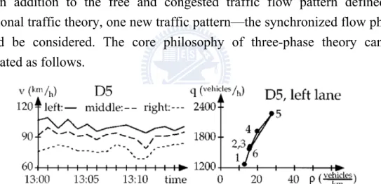
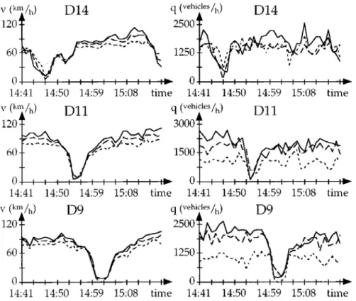
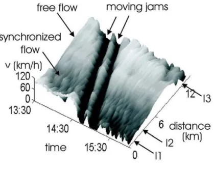
2.6 Three-phase Traffic Theory... 33
2.7 Discussion ... 36
CHAPTER 3 DEVELOPMENT OF REFINED CA MODELS ... 38
3.1 Shortcomings of Existing CA Models... 38
3.2 Common Unit, Cells and Sites ... 41
3.3 Definition of 3-D Generalized Traffic Variables... 44
3.4 Primitive Update Rules for Refined CA Model ... 48
3.4.1 Forward rules... 48
3.4.2 Lane change rules... 51
3.5 Proposed Revision to CA Update Rules... 52
3.5.1 Forward rules with limited deceleration ... 52
3.5.2 Piecewise-linear speed variation ... 54
3.5.3 Revised deceleration mechanism ... 56
3.5.4 Implementation of Newton’s kinematics ... 57
3.5.5 Amendment to vehicular movement ... 59
3.5.6 Revised primitive forward rules... 61
3.6 Description of Numerical Simulation ... 61
3.6.1 Simulation codes ... 61
3.6.2 Concept of OOP ... 62
3.6.3 Description of classes... 64
3.6.4 Simulation flowchart ... 66
CHAPTER 4 LOCAL TRAFFIC DETECTION ... 74
4.1 Local Traffic Parameters ... 74
4.2 Measurement Method... 76
4.3 Arithmetic Averaged versus Un-weighted Moving Averaged Traffic Parameters ... 79
4.4 Simulation Scenarios... 79
4.5 Local Traffic Features ... 80
4.6 Traffic Patterns ... 81
4.6.1 AA traffic data ... 81
4.6.2 UMA traffic data ... 83
4.7 Comparison ... 84
4.8 Summary ... 88
CHAPTER 5 DEVELOPMENT OF SOPHISTICATED CA MODELS ... 89
5.1 Sophisticated CA Rules... 90
5.1.1 Forward rules for cars and motorcycles ... 90
5.1.2 Lateral movement rules for cars... 90
5.1.3 Lateral drift rules for motorcycles... 94
5.1.4 Transverse crossing rules for motorcycles ... 96
5.2 Simulation Results... 97
5.2.1 Pure car simulation... 98
5.2.2 Mixed traffic simulation... 99
5.3 Comparison of Global and Local Traffic Flows ... 106
5.4 Simulation on Signalized Intersections... 109
5.5 Summary ...111
CHAPTER 6 CONCLUSIONS AND RECOMMENDATIONS... 112
6.2 Recommendations ... 117
NOTATION TABLE ... 120
REFERENCES... 123
LIST OF FIGURES
Figure 1-1. Research framework... 6 Figure 2-1. A general description of relationship among fixed control volume,
control surface and a moving system for defining Reynolds
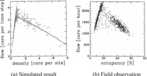
transport theorem. ... 10 Figure 2-2. The theoretical fundamental diagram of traffic... 11 Figure 2-3. Homogeneous cell system utilized in traditional NaSch model. ... 26 Figure 2-4. Comparison of simulated fundamental diagram via NaSch model
with that from the field observation... 26 Figure 2-5. Comparison of simulated x-t plot via NaSch model with that from
field observation. Note the traffic fluctuation induced by one
randomized driver behavior and the its backward movement... 27 Figure 2-6. Field observed x-t diagram of German freeway (A-9, south, dated
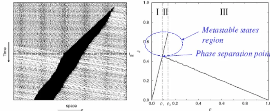
2002.04.26). The vertical axis displays the position along freeway (in kilometer) and horizontal axis as the time marched. (note the parallel movement of traffic jams and the coupled backward speed of traffic jams—15kph approximately.)... 27 Figure 2-7. Simulated x-t diagram (left panel) and fundamental diagram (right
panel) of a spontaneously emerging jam through the VDR model. ... 28 Figure 2-8. Description of hysteresis effect—A local phase transition occurs
from one traffic phase (free flow phase) to another phase
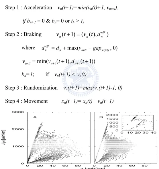
(synchronized flow phase), and later reverses to the initial phase, transforming the hysteresis loop... 28 Figure 2-9. Comparison of the Knopse model (2000, left panel) with empirical
data (right panel)... 31 Figure 2-10. Comparison the fundamental diagrams of three-phases
interpretation (Kerner, 2004, left panel) and that based on real traffic (right panel)... 33 Figure 2-11. Observed flow-density relationships on German highways A-5.
Figure 2-12. Features of free flow phase in three-phase traffic theory... 34 Figure 2-13. Features of synchronized flow phase in three-phase traffic theory.
... 35 Figure 2-14. Upstream propagation of wide-moving jams in three-phase traffic
theory... 35 Figure 2-15. Coexistence of moving jams and their parallel propagation to the
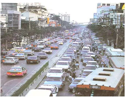
upstream... 36 Figure 3-1. Erratic motorcyclists’ behaviors in congested urban traffic, such as
sneaking into traffic jam and transverse crossing between two adjacent still vehicles. ... 38 Figure 3-2. Comparison between the proposed refined CA grid (i.e., cell/site)
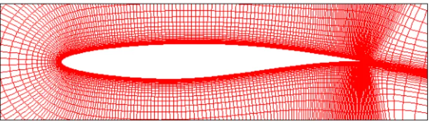
system and that of the traditional CA model for a two-lane roadway context... 42 Figure 3-3. Typical grid generation prevalent in computational fluid dynamics
(CFD) analysis. In this case, 2-D flow field around an airfoil is analyzed. ... 43 Figure 3-4. Definition of 2-D traffic parameters, proposed by Daganzo (1997).
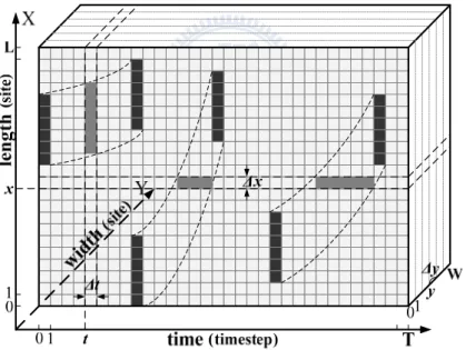
... 46 Figure 3-5. Vehicular trajectories over a specific transverse slice in a
spatiotemporal domain S enclosed byL×W×T. ... 47 Figure 3-6. Lane changes for a car on a two-lane roadway ... 52 Figure 3-7. Unrealistic simulated x-t diagram of primitive CA
model—unlimited deceleration behaviors of vehicles when approaching upstream front of traffic jams. The horizontal axis represents time marched from left to right whereas the vertical axis represents the upward displacement of vehicles... 53 Figure 3-8. Different definitions of vehicular speed update: (a) particle-
hopping variation; (b) piecewise-linear variation... 55 Figure 3-9. Piecewise-linear variation of speed during time interval (t0~t1). ... 60
Figure 3-10. Demonstration of developed C# code; it is constructed upon MS Visual Studio IDE environment... 62
Figure 3-11. User interface of the developed C# simulation code... 64 Figure 3-12. Primary hierarchy of simulation program ... 67 Figure 3-13. Simulated x-t diagram via the revised model, the horizontal axis
represents the time (seconds) passed whereas the vertical axis represents the locations of vehicles. ... 69 Figure 3-14. Zoom-out vehicular trajectories via the revised model when
approaching upstream front of traffic jam. ... 69 Figure 3-15. Comparison of simulated global flow fundamental diagrams of
original and that of the revised model. ... 70 Figure 3-16. The simulated x-t diagrams of same parameters setting (traffic
density 32 veh/km/ln) but with different outcomes. (a) The ideal case, interference among vehicles can hardly be observed. (b) The typical case, a small perturbation incurs dramatic traffic pattern change. ... 71 Figure 3-17. Field observed fundamental diagram (Kerner, 2004), German
highways A-5, daily data 7:00-22:00). Note that the theoretical optimum traffic flow 2,400 veh/hr/ln is seldom found. In most occasions, lower traffic flow prevails and disperses within a certain area in the fundamental diagram... 72 Figure 3-18. Simulated traffic patterns and their transitions (x-t diagrams) for
various traffic densities via the revised CA model. ... 73 Figure 4-1. Four possibilities for a vehicle passing through one stationary
detector for a certain time-step t. ... 77 Figure 4-2. The traffic patterns and flow rate-occupancy relationship. (30s AA
data)... 80 Figure 4-3. The x-t diagram of traffic flow with one bottleneck introduced in
mid-roadway. ... 82 Figure 4-4. Simulation results for light vehicles with bottleneck. (30s AA data)
... 83 Figure 4-5. Traffic patterns and transitions in the downstream of bottleneck.
(30s UMA data) ... 83 Figure 4-6. Traffic patterns and transitions in the upstream of bottleneck. (30s
UMA data) ... 84 Figure 4-7. Comparison of global fundamental diagram with local 1s data for
four different scenarios. (ρ(S)= 0.16, 012, 0.25, 0.50)... 86 Figure 4-8. Comparison of global fundamental diagram with local AA data for
four different scenarios. (ρ(S)= 0.16, 012, 0.25, 0.5)... 86 Figure 4-9. Comparison of global fundamental diagram with local UMA data
for four different scenarios. (ρ(S)= 0.16, 012, 0.25, 0.50)... 87 Figure 5-1. Lateral movements for cars in mixed traffic: lane-change and lateral
drift... 91 Figure 5-2. Gaps evaluated by a car to perform either lane-change or lateral
drift... 93 Figure 5-3. Gaps evaluated by a car to perform lateral drift... 94 Figure 5-4. Field observed motorcycles’ possible movements (Lan and Chang,
2005). ... 94 Figure 5-5. Gaps evaluated by a motorcycle to perform lateral drift from the
middle site... 95 Figure 5-6. Gaps evaluated by a motorcycle to perform lateral drift from the
outermost site... 96 Figure 5-7. Transverse crossing behavior for motorcycles when stuck in traffic.
... 97 Figure 5-8. Fundamental diagrams for cars in pure traffic with and without
introducing lateral drift. ... 98 Figure 5-9. Linear relationship between numbers of cars and motorcycles under
given general densities (ρ(S)). ... 99 Figurr 5-10. Fundamental diagrams for cars in mixed traffic under various C:M ratios... 100 Figure 5-11. x-t plots in mixed traffic with different C:M ratios under car
density ρc =50 veh/km/ln... 100 Figure 5-12. Comparison with existing of fundamental diagrams for cars under
various motorcycle densities (ρm). The horizontal axis represents the preset car density ρc, vertical axis shows the simulated car flow.
... 101 Figure 5-13. Comparison of fundamental diagrams for motorcycles under
various motorcycle densities (ρm) with existing study. The horizontal axis represents the preset car density ρc, vertical axis shows the simulated motorcycle flow... 102 Figure 5-14. Simulated capacity loss suffered from introduction of one
bottleneck in the middle of right lane. Note that a plateau regime may be identified in the mid-density range. ... 103 Figure 5-15. x-t plots in mixed traffic with and without motorcycles’ transverse
crossing behaviors (ρc =100 veh/km/ln, ρm = 10 veh/km/ln). The right panels zoom out the vehicular trajectories in the area marked in the left panels. The designated motorcycle is marked in red... 104 Figure 5-16. Demonstration of simulated trajectories for the designated
motorcycle marked in red in Figure 5-15(b)... 105 Figure 5-17. Comparison of local traffic flow (AA averaged) and global traffic
flow. The left panels depict the derived data for cars and the right panels for motorcycles. ... 107 Figure 5-18. Comparison of local traffic flow (UMA averaged) and global
traffic flow. The left panels depict the data for cars and the right panels for motorcycles. ... 108 Figure 5-19. Preliminary simulation results of one roadway with two signalized
intersections introduced, without and with 30s signal offset. The upper panels show the simulated x-t diagram; the lower panels depict the speed variation of designated vehicle in the upper panels. ... 110
LIST OF TABLES
Table 2-1. Comparison of recommended parameters settings among some famous GM (GHR) models... 17 Table 3-1. Summary of spatiotemporal models (source: Sprott (2003)) ... 56 Table 3-2. Summary of important methods defined for Class CaModelForm . 65 Table 3-3. Summary of important methods defined for Class clsCar ... 66
CHAPTER 1 INTRODUCTION
1.1 Motivation
Understanding vehicular moving behaviors provides the fundamental rationales for planning, designing, controlling and managing the road systems. In order to avoid the time- and money-consuming field observations, numerical implementation can be used as an efficient instead for providing precious reference and guidance. Therefore, along with the rapid progress of digital technology since early fifties, numerous traffic simulation models have been plentifully proposed.
Generally, existing traffic models can be roughly separated into three branches; depending on the level of detail or resolution of traffic been derived—macroscopic, microscopic and mesoscopic models. The coarsest ones are the macroscopic models which include the traffic flow models and fluid-dynamical models. Traffic flow models analyze the relationships between speed, density and volume (May, 1990). Fluid-dynamical models, on the other hand, analogize vehicular flow to fluids and assume that aggregate behavior of drivers is dominated by the surrounding traffic conditions. Lighthill and Whitham (1955) and Richard (1956) developed the most prominent one-order fluid-dynamical models. Subsequently, high-order fluid-dynamical models were developed by other researchers; for example, Payne (1971), Liu et al (1998) and Zhang (1998).
The microscopic traffic flow models, in contrast, describe the interaction between individual vehicle and other vehicles. Car-following models are the most pertinent models to explicate the one-dimensional movements in a longitudinal lane such that the following vehicle adjusts its speed to maintain desirable or safe distance headway to the lead vehicle. Stimulus-response models are perhaps the most prominent models developed in the 1950s and 1960s by the General Motors (GM) research group, because the same principles is still being applied and/or extended nowadays by scholars worldwide, for example, that by May (1990), Brackstone and McDonald (1999), Lan and Yeh (2001), etc.
The third branch, the mesoscopic models, serves as the linkage to fill the gap between the aggregate level approach of macroscopic models and the
individual viewpoint in the microscopic ones. Mesoscopic models aim to describe the behavior of small groups of vehicles. Examples of these models are the cluster models, gas-kinetic models and the cell transmission models. Prigogine & Herman (1971) proposed the kinetic equation of vehicular traffic and summarized the possible alternate forms of the relaxation term. Hoogendoorn and Bovy (1999) proposed a traffic flow model describing multilane heterogeneous (i.e. unconstrained and constrained) traffic flow. Various kinetic models were subsequently proposed by many researchers, such as Paveri-Fontana (1975), Phillips (1979), and more recently Nelson (1995), and Nelson and Sopasakis (1998). Daganzo (1993, 1994) proposed the cell transmission model (CTM model for short) and since then have been popularly utilized for traffic simulation.
Recently, various CA models that can be categorized as one branch from the microscopic perspective have been developed to describe the phenomena of real traffic flows with complex dynamic behaviors, owing to their capacity for reflecting complicated traffic patterns via comparatively concise numerical algorithms. Nagel and Schreckenberg (1992) proposed their famous pioneer model (referred as for NaSch model hereinafter) to reproduce the basic features of real traffic. In their model, the road is divided into squared cells of length 7.5 meters. Each cell can either be empty or occupied by at most one car (i.e., the size of a car is viewed as one cell). Space, speed, acceleration and even time are treated as discrete variables. The state of the road at one certain instant is derived from one time-step ahead by applying acceleration, braking, randomization and driving rules for all cars at the same instant (i.e., parallel dynamics). Obviously, such a coarse description is an extreme simplification of real world conditions; therefore, a considerable number of modified NaSch models has been developed in the past decade. For instance, Nagel (1996, 1998) employed the concept of stochastic CA and treated each particle with randomized-integer speed between zero and maximum speed. Rickert et al (1996) examined a simple two-lane CA model and pointed out some important parameters that define the shape of the fundamental diagram (flow-density); Chowdhury et al (1997) generalized the NaSch model by introducing a particle-hopping model for two-lane traffic with two different vehicle speeds (fast and slow); Barlović et al (1998), in contrast to the constant randomization in the NaSch model, introduced a velocity-dependent randomization (VDR) parameter. Although the VDR model is a simple generalization of the NaSch
model, it is capable of revealing some complex traffic dynamics, i.e., the existence of wide phase separated jams and metastable free-flow states. Nagel
et al (1998) further proposed different CA rules to govern vehicular
lane-change behavior. More Recently, Boris Kerner (2002, 2004), a German traffic physician, introduced a three-phase traffic theory that consists of free flow, synchronized flow, and wide-moving jam phases. The latter two phases exist in congested states in which downstream front of the synchronized flow phase is often fixed at a bottleneck while the wide-moving jam will propagate through the position where bottleneck locates. To explore the emergence of such traffic patterns, Kerner and partners tried to describe the complex spatiotemporal behaviors based on empirical freeway traffic analysis. (Kerner
et al, 2004)
Over the years, most conventional CA models were developed for depicting the traffic phenomena on freeways. However, most of times these models were limited to the simulation of pure traffic scenarios in which vehicles have identical size. Few has been devoted to the analysis of urban traffic such as mixed traffic that is comprised by vehicles in various sizes; such as heavy vehicles (e.g., bus, truck), light vehicles (car) and of course, smaller two-wheel ones (motorcycle, bicycle). It is evidenced that the coarse cell system in existing CA models makes it extremely impossible to reflect various vehicle sizes and the slight speed variation of vehicles on urban streets. Thus inevitably refined cell system must be established beforehand if one ever tries to successfully simulate the urban traffic.
In addition to the refined cell system, some unique behaviors must also be scrupulously considered in places where both cars and motorcycles are introduced. Unlike heavy or light vehicles that normally move within a specific longitudinal lane and sometimes change lanes for overtaking or turning, motorcycles do not move in a specified lane. As the result, conventional flow models may not satisfactorily elucidate the motorcycles’ moving behaviors. Because motorcycles are the most popular transportation mode in Taiwan as well as in some other Asian countries, it is important to gain better insights of the motorcycles’ moving behaviors, from both academic and practical perspectives.
1.2 Research Objectives
The final goal of this study is to develop an effective CA model capable of simulating urban traffic with different vehicle kinds and/or sizes introduced. To fulfill this, the intended multiple purposes of this study can be outlined sequentially as follows.
A To introduce refined grid system to facilitate the implementation of CA into urban traffic simulation
A refined “cell unit” is first proposed for developing the novel CA model. Henceforth, the rules governing the forward movement and lateral shift of vehicles that come into different sizes and their incurred interactions can be conscientiously elucidated. Along with this, the general 3-D traffic parameters, including density, traffic flow and spatiotemporal averaged speed will also be introduced.
B To establish CA update rules for describing vehicular movements
The primitive CA update rules are devised in reference to that proposed in existing CA efforts. In addition, revised CA update rules will be developed to rectify the common defect prevailed in existing CA models, i.e., abrupt deceleration when vehicles encounter stationary obstacles or approach upstream front of traffic jams, as to reflect more precisely the real driving behaviors in real world.
C To define means to measure local traffic parameters
Methodology for deriving local traffic parameters in the proposed refined CA model will be created. Accordingly, macroscopic traffic parameters such as traffic flow, density and speed in various traffic conditions (i.e., with bottleneck, lane-drop, signalized intersection, etc.) can be well derived whereas the local traffic parameters from microscopic approach that describing the incurred complex spatiotemporal traffic patterns and the transitions among them, either on highways or urban streets, can also be obtained.
D To develop sophisticated CA model capable of simulating car/motorcycle mixed traffic
Simulation of various traffic scenarios, such as different car/motorcycle ratios that prevailed in urban streets via the refined CA models will be
implemented. The relevant CA update rules for delineating complicated behaviors of motorcycles will be defined as well. It is expected that some important spatiotemporal characteristics thereof can be successfully obtained.
1.3 Research Framework
To cope with the research purposes, as mentioned, the research framework is demonstrated in the flowchart as shown in Figure 1-1. Each step therein is elaborated in the followings.
(1) Problem identification
The first step is to identify the purposes and scope of this study, and to address problems that need to be explored.
(2) Literature review
The second step is to review related researches in traffic flow theories, including macroscopic, microscopic, mesoscopic models and the car-following theory, especially the existing CA models. This puts the current status of traffic modeling in perspective and identifies the potential defects of existing traffic models that impede their implementation for urban traffic simulation.
(3) Development of basic refined CA models
In this step a refined CA model is proposed, introducing drivers’ heterogeneity into simulation. As the first groundwork, a refined “common
unit” is defined so as to fulfill the required “resolution” for urban traffic
simulations. Along with that, several spatiotemporal traffic parameters are thereby devised. Second, referring to traditional CA models, some basic forward and lane-change rules that govern vehicular movements are developed. The refined CA model, coupled with these basic CA update rules, is capable of capturing the essential features of traffic flows, including those found in previous works. Thirdly, to cope with the real vehicular performance behavior with required precision, the basic model is extended further to mandate vehicles equipped with piecewise linear speed variation as well as limited deceleration capacity. It shows that this amendment can reflect the genuine driver behavior in real world and is capable of revealing Kerner’s three-phase traffic patterns. By end of this step, the methodology for deriving local traffic parameter in the proposed refined CA model will also be developed.
(4) Development of sophisticated CA models
Upon the refined CA model developed in step 3, simulations for mixed traffic with diverse compositions of cars and motorcycles are carried out. For this, CA update rules, especially lateral movement update rules besides the lane-change rules, must be addressed according to the attributes of each individual vehicle and the traffic situations around it. Therefore a
sophisticated CA model to elucidate the erratic motorcycle behavior in mixed traffic contexts is devised. In addition to the conventional moving forward and lane-change rules, the sophisticated CA model also explicates the lateral drift behavior for cars moving in the same lane, the lateral drift behavior for motorcycles breaking between two moving cars, and the transverse crossing behavior for motorcycles through the gap between two stationary cars in the same lane. Fundamental diagrams and space-time trajectories for vehicles with various car-motorcycle mixed ratios are demonstrated and compared with existing effort..
(5) Conclusions and recommendations
After the exhaustive and deliberate explorations, the findings in the model formulation and validation will be summarized. The strengths and weaknesses of the proposed model will then be discussed, followed by some recommendations for future study.
1.4 Chapters Organization
This thesis is organized as follows. Chapter one briefly describes existing traffic flow models and illustrates the motives for proposing the new CA model, followed by a brief circumscription of research objectives, research framework of this study. Chapter two overviews previous works and the diverse existing traffic flow models, especially the progress of CA models in latest two decades. Chapter three examines first the main defect of existing CA models, in particular, the deficiency for urban traffic simulation is pointed out and the potential cause is discussed; following is a detail illustration of the developed refined CA model. Chapter four describes the methodology for measuring local traffic parameters via the proposed CA model. Chapter five further proposes the sophisticated CA model for mixed traffic comprised by cars and motorcycles. Chapter six summarizes, concludes and addresses issues for future studies.
CHAPTER 2 LITERATURE REVIEW
Conventional traffic flow models can be roughly separated into macroscopic, microscopic and mesoscopic models, as the level of detail in simulation ranges from the coarsest to the finest, respectively. Macroscopic models describe traffic flow as fluid flow and hence analyze traffic phenomena at a high level of aggregation (for example, number of vehicles per hour that pass a certain spot) without considering its constituent parts (the vehicles), Microscopic models describe the behaviors of the entities making up the traffic flow (the vehicles) as well as their interactions in detail. On the other hand, mesoscopic models are at an intermediate level of detail, oftentimes aiming at description of vehicles in groups instead the interactions among individual vehicles. All these approaches, especially the prominent car-following theory and related vehicular traffic theory are reviewed in this chapter.
2.1 Macroscopic Approaches
Macroscopic traffic models were virtually originated from fluid dynamics in which traffic flow is treated as continuous chain and behaves analogous to fluid flow. Thus, the continuity equation for traffic flow can be derived via the well-known Reynolds transport theorem. Therefore, relationship among some important traffic parameters, such as traffic flow, density and average speed from global perspective can be derived. The basic philosophy thereof, the renowned law of conservation of mass flow, is illustrated as below.
2.1.1 Conservation law for traffic flow
The general form of Reynolds transport theorem that familiar to scholars in fluid dynamics field is enclosed as Equation 2-1.The LHS of Equation (2-1) represents the variation rate of a moving system B at time-step t from Lagrangian viewpoint (i.e., a coordinate system following the movement of system B), whereas the RHS thereof represents the summation of variations inside a fixed control volume (CV) and the influx/outflux across the control surface (CS) at same time-step, i.e., from Eulerian viewpoint, as shown in Figure 2-1. The parameter b is defined as elementary unit of system B.
∫∫
⋅ +∂∂∫∫∫
= cs cv dV b t dA V b Dt DB ) ( ) (ρ ρ (2-1) where∫∫∫
= system dV b B ρ (2-2)When B is set as mass (or say, b equals to unity), and the mass of system
B is assumed to be unchanged (in traffic theory, this implies that there is no
vehicular exit or access for system B), Equation (2-1) is transformed into the so-called equation of conservation for mass flow—the continuity equation, shown as Equation (2-3). 0
∫∫
∫∫∫
+ ⋅ = ∂ ∂ cs cv dA V dV t ρ ρ (2-3)Figure 2-1. A general description of relationship among fixed control volume, control surface and a moving system for defining Reynolds transport theorem.
2.1.2 Lighthill-Whitham-Richards (LWR) model
For traffic prevailed on freeway, since longitudinal movement is the main concern, the continuity equation is further simplified into a two-dimensional equation with two independent variables—location x at an instant of time t. Upon this, Lighthill and Whitham (1955) first conjectured that density is the function of the two above-mentioned independent
variables—ρ=ρ(x,t). After that, they adopted the traditional formula for estimating fluid flow rate q (Equation 2-4). Thus the continuity equation in form of first order partial differential equation (PDE) can be derived as Equation (2-5): q= ρv (2-4) 0 ) , ( ) , ( = ∂ ∂ + ∂ ∂ x t x q t t x ρ (2-5) An additional hypothesis was inspired by the q-ρ profile from the theoretical fundamental diagram of traffic (FD, see Figure 2-2) to assume that flow is the function of density only (Equation (2-6)); therefore Equation (2-5) can be reduced as Equation (2-7).
q=q(ρ) (2-6) 0 )) , ( ( ) , ( = ∂ ∂ + ∂ ∂ x t x q t t x ρ ρ (2-7) flo w r ate density slope v
Figure 2-2. The theoretical fundamental diagram of traffic.
Since now there is only one dependent variable—the vehicles’ density ρ in the derived equation; it becomes possible to obtain the analytic solution of this PDE if its initial and boundary conditions are both given and, finally leading to a solvable traffic flow model.
In the LWR theory, a traffic disturbance is propagated by kinematic waves at a speed
Kinematic waves (KW) ρρ
d dq
c= ( ) (2-8) According to Equation 2-8 and Figure 2.2, one can find that the KW velocity is positive on the part of the fundamental diagram where the flow rate
increases with density, and it is negative on the part of the fundamental diagram where the flow rate decreases with density.
Besides the effort of Lighthill and Whitham, one year later Richards (1956) published a similar model. Therefore, this model is usually referred to as the Lighthill-Whitham-Richards (LWR) model.
2.1.3 Other macroscopic models
Obviously LWR model is an over-simplification of traffic phenomena, since it assumes a homogeneous and deterministic traffic flow and it implies smooth and concave functionso for both speed and density. Therefore in the past three decades, many efforts were devoted in improving the LWR model. Most notable studies in this regard include the work by Bick and Newell (1960) for two-lane bidirectional road, by Munjal and Pipes (1971) for multi-plane freeways and those by Liu et al (1998) and Zhang (2005) of high-order similar models. In the same spirit, some other proposed systems of finite different equations (FPE) to model freeway traffic, such as Payne (1971) and Daganzo (1995). Wong and Wong (2002) further formulated a multi-class traffic flow model as an extension of LWR model with heterogeneous drivers.
2.2 Mesoscopic Approaches
Mesoscopic models bridge the gap between macroscopic and microscopic models by combining the aggregate traffic flow variables with some assumptions on the interactions among vehicles. Mesoscopic models normally describe the traffic entities at a high level of detail whilst their behaviors and interactions are described at a lower level of detail.
The mesoscopic models can take varying forms. One form is vehicles grouped into packets, which are routed through the network (Leonard et al, 1989). Each packet of vehicles acts as one entity and its speed on each road (link) is derived from a speed-density function defined for that link as well as the density on the link at the moment of entry. The density on a link is defined as the number of vehicles per kilometer per lane. A speed-density function relates the speed of vehicles on the link to the density.
The second approach is the gas-kinetic traffic models. Analogous to gas kinetic theory, in these models traffic flow is treated as a gas of interacting
particles where each particle represents a vehicle. As such, instead of describing the traffic dynamics of individual vehicle, gas-kinetic traffic flow models describe the dynamics of the velocity distribution functions of vehicles in the traffic stream. Recent application of gas-kinetic traffic flow models can be referred to Hoogendoorn (1999) and Klar & Wegener (1999).
Another mesoscopic paradigm is that vehicles are grouped into cells which control their behaviors. The cells traverse the link and vehicles can enter and leave cells when needed, but not to overtake. The speed of the vehicles is determined by the cell, not the individual driver’s decision. One famous approach in this regard is the cell transmission (CTM) model proposed by Daganzo (1993, 1994). In that, the LWR continuum model is discretized into cells. The road is represented by a number of small sections (cells). The simulation model keeps tracking the number of vehicles in each cell, and in each time-step it calculates the number of vehicles that cross the boundaries between adjacent cells. The flow from one cell to the other depends on how many vehicles can be sent by the upstream cell and how many can be received by the downstream cell. The amount of vehicles that can be sent is a function of the density in the upstream cell whereas the number can be received depends on the density in the receiving cell. The lagged cell transmission model (Daganzo, 1999) is a refinement of this scheme, where the amount of vehicles a cell can receive (from the adjacent upstream cell) is also affected by the density some time earlier in the cell.
One new category in this regard is the hybrid model which tries to introduce concurrently the macroscopic and microscopic model into simulation. For example, Leclercq and Moutari (2007) proposed to take the advantage of different approaches and tried to develop a combined algorithm which includes both macroscopic model (based on Eulerian coordinate) such as LWR model and the microscopic model (based on Lagrangian coordinate) in order to provide more efficient traffic simulations on large road networks. However, they agreed that there are two important questions have to be addressed first when developing a hybrid model: (a) How closely are the microscopic and macroscopic models to be coupled? (b) How to synchronize or to translate boundary conditions, when passing from one traffic representation to another? For this they also tried to define the translations of boundary conditions at interfaces in the primitive hybrid model they proposed.
2.3 Microscopic Approaches
The microscopic models describe the interrelationship of individual vehicle’s movement as well as its interaction with other vehicles. In these models of vehicular traffic, attention is focused on individual vehicle that is represented by a “particle”. Car-following models are the most pertinent ones to explicate the one-dimensional movements in a longitudinal lane such that the following vehicle adjusts its speed to maintain desirable or safe distance headway to the lead vehicle. Stimulus-response model is perhaps the most prominent one developed in the 1950s and 1960s by the General Motors (GM) research group, which is still being applied or extended (e.g., Brackstone & McDonald, 2000; Chakroborty & Kikuchi, 1999; Lan & Yeh, 2001). The car-following models are summarized as follows.
2.3.1 Concept of “car following”
The terminology “car following” on a motorway means the behavior of a driver who, through control of the brake and accelerator, tends to maintain an acceptable distance behind the lead vehicle in the same lane. Therefore, for each individual vehicle, an equation of motion is defined, which is the analogue of the Newton's equation for each individual particle in a system of interacting particles. In Newtonian mechanics, the acceleration may be regarded as the response of the particle to the stimulus it receives in the form of force which includes both the external force as well as those arising from its interaction with all the other particles in the system.
2.3.2 Stimulus-response relationship
The basic philosophy of the car-following theories can be summarized by the relationship:
n
n stimulus
response] [ ]
[ ∝ (2-9) Each driver can respond to the surrounding traffic conditions only by accelerating or decelerating the vehicle. Different equations of motion were proposed in various car-following models, arising from their differences in postulating the nature of stimulus. In general, the Newtonian kinetics is adopted as the basic principle for movement:
) , , ( n n n sti n f v x v x&& = Δ Δ (2-10)
where the function fsti represents the stimulus received by the nth vehicle.
Different car-following model interprets the function fsti differently. In the
following, several car-following models are illustrated.
2.3.3 Pipes’ car-following theory
The very first car following model can be traced back to the primary model proposed by Pipes (1953). He introduced the concept of minimum (safety) space headway, as shown below:
∆xn(t) = (∆x)safe +τ*vn(t)= xn+1(t) - xn(t) (2-11)
where τ is a parameter that sets the time scale of the model
) ( ) (t x. t
vn = n is the speed of nth vehicle at instant t
n+1 represents the vehicle in right front
Accordingly, one may derive the acceleration/deceleration of each vehicle by differentiating, with respect to time, on both sides of the Equation (2-11). )] ( ) ( [ 1 ) (t x 1 t x t x&&n = &n+ − &n
τ (2-12) This model encapsulates two basic assumptions: (a) The higher the speed of the vehicle the larger should be the distance-headway. (b) In order to avoid collision with the lead vehicle, each driver must maintain a safe distance
(∆x)safe to the lead vehicle. Therefore, in Pipes models, both the coefficients of
the general form (refer to the Equation (2-18), shown as below) are set as
m=l=0. According to Pipes, (∆x)safe=20ft and τ =1.36 s.
2.3.4 Forbes’ car-following theory
Forbes (1958) approached the car-following behavior by considering the reaction time needed for the following vehicle to perceive the need for decelerating and applying brakes. The final formula proposed, however, is identical to that (Equation (2-12)) in Pipe’s model but still with slightly difference, i.e., (∆x)safe=20ft and τ =1.5 s.
The five-generation GM model (1960, also known as GHR model owe to the contribution made by Gazis, Herman and Rothery in late fifties and early sixties, or the follow-the-leader model) is perhaps the most well known model. Its general formulation is:
) ( * ) ( ) ( * v t T T t x t v stimulus y sensitivit x l m n n ∝ = Δ − Δ − α && (2-13)
where T is the reaction time.
The first prototype car-following model that would eventually lead to general GM formula was put forward in the late 50s by Chandler, Herman and Montroll (1958) at the General Motors research labs in Detroit, MI. This was based on an intuitive hypothesis that a driver's acceleration was proportional to the relative speed to the front vehicle (∆v), or a deviation from a preset following distance. Also for a more realistic description, the strength of the response of a driver at time t should depend on the stimulus received from the other vehicles at time t-T, where T is a response time lag. Hence, an equation known as the GM#1 model that similar to Equation (2-12) is derived:
)] ( ) ( [ ) (t T x 1 t x t
x&&n + =α &n+ −&n GM#1 model (m=0, l=0) (2-14) Where α is the sensitivity coefficient, an experimental constant independent of n, and α varies from 0.17~0.74.
The second generation GM model was proposed later by the same research team in light of the fact there are different driving behaviors for drivers stuck in the platoon. So the sensitivity coefficient α is divided into following two groups:
)] ( ) ( [ ) (t T x 1 t x t
x&&n + =αi &n+ − &n GM#2 model (m=0, l=0) (2-15)
Where i=1 or 2, α1 is the coefficient for driving in platoon and α2 is the
coefficient for driving not in platoon.
Gazis, Herman and Potts (1959) subsequently attempted to derive a macroscopic relationship describing speed and flow; using the microscopic equation as a starting point. The mismatch between the macroscopic relationship they obtained and the other macroscopic relationships in use at that time led to the hypothesis that the algorithm should be amended further by
introducing a 1/∆x term into the sensitivity constant (i.e., α Æ α/∆x), in order to
minimize the discrepancy between the two approaches. This led to the third generation GM model: )] ( ) ( [ ) ( ) ( ) ( 1 1 0 x t x t t x t x T t x n n n n n & & && ⎢ − ⎣ ⎡ ⎥ ⎦ ⎤ − = + + + α GM#3 model (m=0, l=1) (2-16)
Subsequently, Edie (1960) attempted to match the m=0, l=1 model to new macroscopic data in a similar manner to Gazis, Herman and Potts. However, he concluded that another amendment should be made to the sensitivity constant, namely, the introduction of the velocity dependent term. This produced a new model with m=1 and l=1:
)] ( ) ( [ ) ( ) ( ) ( ) ( 1 1 0 x t x t t x t x T t x T t x n n n n n
n & & &
&& ⎢ − ⎣ ⎡ ⎥ ⎦ ⎤ − + = + + + α GM#4 model (m=l, l=1) (2-17)
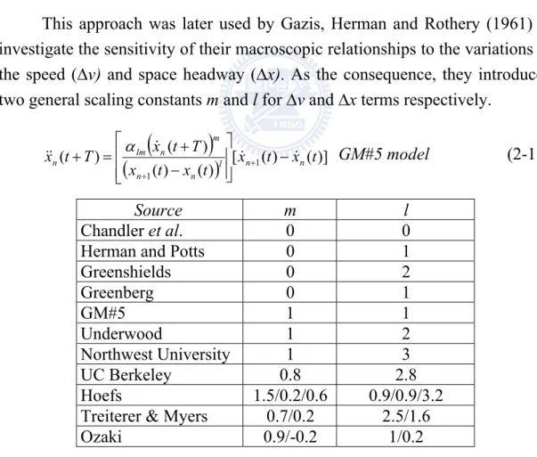
This approach was later used by Gazis, Herman and Rothery (1961) to investigate the sensitivity of their macroscopic relationships to the variations of the speed (∆v) and space headway (∆x). As the consequence, they introduced two general scaling constants m and l for ∆v and ∆x terms respectively.
(
)
(
( ) ( ))
[ ( ) ( )] ) ( ) ( 1 1 t x t x t x t x T t x T t x l n n n n m n lmn & & &
&& − ⎢ ⎢ ⎣ ⎡ ⎥ ⎥ ⎦ ⎤ − + = + + + α GM#5 model (2-18) Source m l Chandler et al. 0 0 Herman and Potts 0 1
Greenshields 0 2 Greenberg 0 1 GM#5 1 1 Underwood 1 2 Northwest University 1 3 UC Berkeley 0.8 2.8 Hoefs 1.5/0.2/0.6 0.9/0.9/3.2 Treiterer & Myers 0.7/0.2 2.5/1.6
Ozaki 0.9/-0.2 1/0.2
Table 2-1. Comparison of recommended parameters settings among some famous GM (GHR) models
Thus the generalized formula of GM model was derived. Numerous investigations occurred during the following 15 years, in the attempt to derive
the “best” combination of m and l. However, since the late 70s' the GM model has seen less and less frequently investigated and used, perhaps suffered from the large number of contradictory findings as to the correct values of m and l. These contradictory findings may be caused by two facts. First, the follower’s behavior is likely to vary in accordance with different traffic condition around it; analysis from microscopic perspective has confirmed this argument in part. Second, many of the empirical investigations were taken place at low speeds or in some extreme stop-start conditions, which may not reflect the general car-following behavior. Nevertheless, some famous models in this regard that may be considered to contribute are enclosed in Table 2-1.
2.3.6 Optimal velocity (OV) models
Bando et al (1995) assumed that each driver tends to maintain a safe distance to the lead vehicle by choosing a proper speed as his/her desired speed: )] ( ) ( [ 1 ) (t x t x t x desired n n n n & & && =τ − (2-19) where desired n
x& is the desired speed of the nth driver at time t.
Bando et al (1998) further assumed that the desired speed depends on the distance headway of the nth vehicle.
)) ( ( ) (t x x t x opt n n desired n = & Δ & (2-20) where xopt( xn(t)) n Δ
& is the optimal speed, so that
)] ( )) ( ( [ 1 ) (t x x t x t x opt n n n n & & && =τ Δ − (2-21)
The performance of OV model depends intensively on the appropriate choice of the optimal velocity function (Equation (2-20)). Through introduction of appropriate optimal velocity, such as Heaviside step function, some important macroscopic characteristics, such as traffic jam and hysteresis effects (refer to Figure 2-8 herein below for description) can be observed.
The main weakness of OV model is that under certain conditions the analytic solution, even for homogenous flow, becomes unstable and thus limits the applicability to mixed flow. The second key impediment is that it is
difficult to specify appropriate optimal velocity function for different traffic condition (e.g., free flow or congested flow).
2.3.7 Safety distance (SD) or collision avoidance models
Also known as “collision avoidance” model, the original formulation of
“safety distance” model can be dated back to Kometani and Sasaki (1959).
Their primary methodology does not describe a stimulus-response type function as proposed by the GM model, but seeks to specify a safe following distance through the manipulation of the basic Newtonian equations of motion, in case the vehicle in front were to act “unpredictably”. The full original formulation is as follows:
∆x(t-T) =αxn-12(t-T) + β1vn2(t) + βvn(t)+ b0 (2-22)
The coefficients T, α, β1, β, b0 were determined from the calibration data
from either a pair of test vehicles on city streets or from a test track. However, it is found that the coefficients vary for different occasions and along that, led to different R2 values (0.25 and 0.95 respectively).
A major development of this model was made by Gipps (1981), in which he considered several mitigating factors that the earlier formulation neglected. These were that drivers will allow an additional “safety” reaction time equal to
T/2, (it can be shown that this condition is sufficient to avoid a collision under
all circumstances), and that the kinetic terms in the above formula are related to braking rates of 1/2bn, where bn is the maximum braking rate that the driver of
the nth vehicle wishes to use. Gipps offered no calibration of his parameters, but instead performed simulations showing that his model produced realistic behavior on the propagation of disturbances, both for a vehicle pair and for a platoon of vehicles.
Since the effort of Gipps was published, the SD model continues to be widespread adopted as the simulation model. Part of the attractiveness of this model is that it may be calibrated using common sense assumptions about driver behavior, needing (in the most part) only the maximal braking rates a driver will use and the expected behavior of other drivers, to make it to be fully functional.
Although it produces acceptable results as, for example, comparing the simulated propagation of disturbances against empirical data, there are still some problems that cannot easily be solved. For example, if one examines the
“safe headway” concept, it would not be a totally valid starting point, as in
practice a driver may consider conditions several cars down stream, basing his assumption of how hard the vehicle in front will decelerate on the “preview
information” obtained.
2.3.8 Linear (Helly) models
The original formulation of this approach dated to Helly (1959). He proposed a model that included additional terms for the adaptation of the acceleration according to whether the vehicle in front (and the vehicle two in front) was braking. The simplified model is shown as the following Helly equation:
an(t)= C1∆v(t-T) + C2(∆x(t-T) - Dn(t)) (2-23)
where
Dn(t)=α + βv(t-T) + γan(t-T) ;D(t) is a desired following distance.
From late fifties to early nineties, there are several researches published in this regard proposing the optimal parameter combination for Helly equation.
A major strength of the Helly model is the specific incorporation of
“error”, an element of the original formulation that is often overlooked. And
some linear models (e.g. the model proposed by Xing, 1995) give an extremely good fit to the observed vehicle trajectories. However, criticism applied to the GM model can also be applied to the linear model, i.e., significantly contradictory findings as to the correct values of coefficients C1and C2.
2.3.9 Psychophysical or action point (AP) models
The first model of this category was proposed by Michaels (1963), who raised the concept that drivers would initially be able to tell they were approaching a vehicle in front, primarily due to changes in the apparent size of the vehicle, by perceiving relative velocity through changes on the visual angle (θ) subtended by the vehicle ahead. The threshold for this perception is well-known in perception literature and given as ∆v/∆x2~6*10-4. Once this
threshold is exceeded, drivers will chose to decelerate until they can no longer perceive any relative velocity and the threshold is not re-exceeded. This model in essence is based upon the theory that drivers’ actions rely on whether they can perceive any changes in spacing.
The second model in this regard which introduced spacing-based threshold (generically termed an “action point”) is particularly relevant at close headways where speed differences are always likely to below threshold. Thus, for any changes to be noticeable, ∆x must be replaced by a “just
noticeable distance” (JND), related to Webers Law. This means that the visual
angle must change by a set percentage; typically 10%. It is also noted that this threshold is ~12% for the opening situation, which implies that a driver continually approaches and then moves back from the vehicle in front.
It is important to state that in crossing this last threshold, the driver will set a determined acceleration/deceleration and stay with it until they break another threshold, as the driver perceives no change in conditions, or at very least, no change in the rate of change. It is also likely that in this close-following area the driver is not fully able to control the acceleration/deceleration of his vehicle, due to the very fine adjustments required. Motion is therefore governed by the use of a minimum value.
The next advance of these models came through a series of perception-based experiments conducted in the early seventies, by researchers such as Evans and Rothery (1973) and by the staff at If V Karlsruhe in Germany in the eighties. However, more recent work by Reiter (1994) in which an instrumented vehicle was employed to measure the action points has resulted in the amendment of some of these parameters and led to a totally different functional form, as compared with previous ones.
Besides, although the entire system would seem to simulate behavior acceptably, calibration of the individual elements and thresholds has been less successful. For example, since the sixties, little research work has been undertaken on the concepts involved in these models. It is difficult therefore to either prove or disprove the validity of this model, although the basis upon which it is built is undoubtedly the most coherent, and best able to describe most of the features that we see in everyday driving behavior.
2.3.10 Fuzzy logic-based models
The use of fuzzy logic within car-following models is worthy of mention as it represents the logical step in the attempt to accurately describe driver behaviors. Such models typically divide their inputs into a number of overlapping “fuzzy sets” whereas each set describes how adequately a variable fits the description of a “term”. For example, a set may be used to describe and quantify what is meant by the term “too close”, where for example a separation of less than 0.5s is definitely “too close” and thus has a degree of truth or
“membership” of 1, while, a separation of 2s is not close and is given a
membership of 0, and intermediate values are said to exhibit “degrees” of truth and have differing (fractional) degrees of membership. Once defined, it is possible to relate these sets via logical operators to equivalent fuzzy output sets (e.g., IF “close” AND “closing” THEN “brake”), with the actual course of action being assessed from the modal value of the output set, calculated as the sum of all the potential outcomes.
The initial use of this method (Kikuchi & Chakroborty, 1992) attempted to “fuzzify” the traditional GM model; using ∆x; ∆v and acceleration as inputs and grouping them into several natural-language based sets. This model has been used to illustrate how the fuzzy logic system can be used to describe car following, and the outcome was compared with that from the traditional GM models. It is demonstrated that the GM model would produce differing headways according to the rate of deceleration and hence the final speed. This is clearly in contradiction to what would be expected in practice. Additionally, the final following distance was shown to be dependent only on final speed, regardless of the original following distance or original speed.
Although this model generally reflects the changes expected, its formulation is unrealistic for two reasons. The acceleration of a vehicle can be detected (it is highly debatable whether this is possible), and it has been found from the linear (Helly) model that any linear dependence on ∆x is exceedingly small.
Other work in this area includes that by Teodorović (1994), Ho et al (1996) and work by Yin et al (2002). However, none of these approaches have attempted to calibrate the most important part of the model itself—the membership sets.
2.4 Cellular Automaton (CA) Models
CA modeling, also a microscopic approach, is one powerful tool for traffic simulation; owing to its inherent simplicity and the capacity of reproducing important entities prevailed in real traffic, e.g., density-flow relation and the backward movement of traffic jams in congested traffic. As the consequence, it is not surprised that since early nineties it is popularly utilized worldwide to describe the phenomena of real traffic flows characterized with complex dynamic behaviors.
Besides its inherent simplicity and efficiency, CA models also furnish an important advantage as compared with other car-following models—the ability for simulating multi-lane traffic. Most microscopic car-following models endeavored at delineating drivers’ reaction to the traffic situation in front whilst few ever tried to take care of the traffic condition aside. As the result, in most car-following models only single lane traffic contexts were considered. Since in real world traffic is usually composed by vehicles with different desired speed (in other word, drivers with heterogeneous attributes), introducing different vehicle attributes in a single lane model will inevitably result in platoon in which slow vehicles are followed by faster ones and the average speed is reduced to the free-flow speed of the slowest vehicle (Nagel et al, 1998). It is apparent that such single lane models are not capable of modeling heterogeneous traffic contexts.
Besides, in real world most road systems are comprised of at least two-lanes, thus allow vehicles to change lane, or say, move sideway to overtake a slow vehicle in the front. Consequently, the lane-changing rules that can reflect the driving behaviors must be delineated if one intends to simulate the traffic on multi-lane road contexts. However, as above-mentioned, the car-following models lack the applicability for describing lane change behaviors and hence the multi-lane contexts. In contrast, through the combination of CA models and well-defined lane change rules, simulation of the multi-lane traffic becomes practicable. This might explain its predominance to other car-following models in the past two decades.
Cremer and Ludwig (1986) proposed a simple model which simulated vehicular traffic on the basis of Boolean operations. Several years later, Nagel and Schreckenberg (1992) proposed the renowned NaSch model. Although its