模擬雙向貼圖函數材質上漆之效果

國

立

交

通

大

學

資訊科學與工程研究所

碩

士

論

文

模 擬 雙 向 貼 圖 函 數 材 質 上 漆 之 效 果

Simulating the Painted Appearance of BTF Materials

研 究 生：陳達恩

指導教授：莊榮宏 教授

林文杰 教授

模擬雙向貼圖函數材質上漆之效果

Simulating the Painted Appearance of BTF Materials

研 究 生：陳達恩 Student： Ta-En Chen

指導教授：莊榮宏 Advisor： Jung-Hong Chuang

林文杰 Wen-Chieh Lin

國 立 交 通 大 學

資 訊 科 學 與 工 程 研 究 所

碩 士 論 文

A Thesis

Submitted to Institute of Computer Science and Engineering College of Computer Science

National Chiao Tung University in partial Fulfillment of the Requirements

for the Degree of Master

in

Computer Science

February 2011

Hsinchu, Taiwan, Republic of China

i

模擬雙向貼圖函數材質上漆之效果

研究生 : 陳達恩 指導教授 : 莊榮宏 博士

林文杰 博士

國立交通大學

資訊學院資訊科學與工程研究所

摘 要

Simulating the Painted Appearance of BTF Materials

Student: Ta-En Chen

Advisor: Dr. Jung-Hong Chuang

Dr. Wen-Chieh Lin

Institute of Computer Science and Engineering

College of Computer Science

National Chiao Tung University

ABSTRACT

The Bidirectional Texture Function (BTF) is a very realistic material representation, but it does not offer the user good control and editability over the data. Users can not change the BTF data in a simple and effective way. We present a method for simulating the painted appearance of a material that is represented by the Bidirectional Texture Function. We first transform the image-based BTF into a simple representation that is composed of a height-field and a spatially varying bidirectional reflectance distribution function (SVBRDF). This representation allows us to simulate the appearance of paint on the surface and to estimate the reflectance of the material after being painted. During rendering, we combine a currently existing BTF rendering tech-nique and the modified material data to simulate the painted appearance of the BTF material. Our experiments show that the proposed approach can change the material appearance while preserving the impressions and feelings of the original BTF.

Acknowledgments

I would like to thank my advisors, Professor Jung-Hong Chuang, and Wen-Chieh Lin for their guidance, inspirations and encouragement. Thanks to my colleagues in CGGM lab: Jau-An Yang, Hong-Xuan Ji, and Cheng-Min Liu for going through these years with me, Jyh-Shyang Chang, Yueh-Tse Chen, Ying-Tsung Li, Hsin-Hsiao Lin, Kuang-Wei Fu, and Tsung-Shian Huang for their technical assistances and encouragements, Ying-Yi Chou, Chia-Ming Liu, Chien-Kai Lo, Yu-Chen Wu, Yun Chien, and many others. Special thanks go to Yu-Ting Tsai for generously sharing his work with me and giving me useful advices. I would also like to thank all the brothers and sisters in the Churches in Hsinchu and Taipei for their kindly care and all the prayers for me. Lastly, I would like to thank my parents for their unconditional love, patient, and support. Thank God for loving me and giving me the experience that I have gone through these years.

Contents

1 Introduction 1

1.1 Contributions . . . 2

1.2 Outline . . . 3

2 Related Work 4 2.1 BTF Compression, Rendering, and Editing . . . 4

2.1.1 BTF Compression and Rendering . . . 4

2.1.2 BTF Editing . . . 6

2.2 Paint and Its Rendering . . . 6

3 Approach 9 3.1 Framework . . . 9

3.2 Height Field and SVBRDF Reconstruction . . . 11

3.2.1 Height Field and Normal Map Reconstruction . . . 11

3.2.2 SVBRDF Fitting . . . 13

3.3 Painting Effects on Height Field and SVBRDF . . . 17

3.3.1 Apply Paints on Height Field and Normal Map . . . 17

3.3.2 The Paint Model . . . 17

3.3.3 Apply Paints on SVBRDF . . . 19

3.4 Rendering . . . 20 iii

4 Results 23 5 Conclusion 43 Bibliography 45

List of Figures

2.1 Light behavior in paint. . . 8

3.1 Method Framework. . . 10

3.2 Original BTF image, reconstructed height field and normal map. . . 13

3.3 Gather all measurements of a texel into a single file. . . 14

3.4 The SVBRDF fitting process. . . 15

3.5 Plane parallel layers. . . 18

3.6 The S and K coefficients from [CAS+97]. . . 21

4.1 Comparison between original BTF images and fitting results. . . 25

4.2 Another comparison between original BTF images and fitting results. . . 26

4.3 Original BTF images and the painted results. . . 27

4.4 Original BTF images and the painted results. . . 28

4.5 Painted BTF v.s. alpha blending. . . 29

4.6 Painted BTF v.s. alpha blending. . . 30

4.7 A comparison between renderings using local PCA and using only the recon-structed information. . . 32

4.8 A comparison between renderings using local PCA and using only the recon-structed information. . . 33

4.9 A splash pattern with different watercolor paints on a lizard model. . . 35

4.10 A splash pattern with different oil paints on a lizard model. . . 36

4.11 A flower pattern with different refractive indices on a cloth model. . . 37

4.12 A flower pattern with different refractive indices on a cloth model. . . 38

4.13 Results of a paint brush pattern. . . 39

4.14 Results of a paint brush pattern. . . 40

4.15 Multiple paint layers. . . 41

4.16 Multiple paint layers. . . 42

C H A P T E R

1

Introduction

To produce realistic rendering, which is a main goal of computer graphics researches, we need to have good material representations. While simple materials can be represented by the bidirectional reflectance distribution functions (BRDF), complex materials that have detailed mesostructures can be represented by the bidirectional texture functions (BTF) [DVGNK99]. These detailed mesostructures produce subtle lighting effects such as self-shadowing, inter-reflections, and masking. A BTF is a 6D function which depends on position, the lighting direction, and the viewing direction. Since it is essentially captured from real materials, it can produce very realistic imagery, though it still has drawbacks that are mainly elaborate measure-ment process, the storage requiremeasure-ment, and the lack of control over the sampled data. There have been lots of researches concerning the capturing, modeling, compression, and synthesis of BTF data, while some papers develop methods to edit them.

Recently, some researches expand the BTF to contain an additional time dimension to model the physical or chemical process of materials [GTR+_{06]. But this would require not only}

cap-turing the data once but many times. Therefore we would like to find a way that allows us to simulate some real world process on the image-based BTF data, producing realistic results

1.1 Contributions 2 while omitting the time-consuming capturing process. More specifically, we want to paint on a material that is represented by BTF.

Since BTF is image-based, it does not contain any physical information of the material, such as geometry or reflectance, there is no straight forward way to model any physical or chemical process of the BTF material. Although there are methods proposed to edit the BTF data, they are not able to solve our problem completely. The method we proposed is roughly as follows. We first extract approximate geometry and reflectance information of the material, so that we can simulate the flowing of paint on the material and estimate the reaction of the painted material to incident light. The flowing of paint can be simulated by any suitable fluid dynamics simulation algorithm while the reflectance of the painted surface is estimated by the Kubelka-Munk model. The rendering of the material is seperated into two parts, the painted part and the unpainted part. For the painted part, we gather all the modified geometry and reflectance information to calculate the painted material appearance. For the unpainted part, we adapt a currently existing BTF rendering technique so that the detail information encompassed in the original BTF data is preserved. By using current graphics hardware, we are able to present the result in an interactive speed.

1.1

Contributions

The contributions of this thesis can be summarized as:

• An integrated solution for simulating painting effects on a BTF material is proposed. • The Kubelka-Munk reflectance model is combined into the solution to achieve a new

effect simulating a real world process.

• A hybrid rendering method displaying the original and modified data at the same time in an interactive rate.

1.2 Outline 3

1.2

Outline

The rest of the thesis is organized as follows: Chapter 2 gives a background review on BTF compression, modeling, and editing, and also a review on paint rendering. Chapter 3 illustrate the framework and details of our proposed method. Chapter 4 shows the results of our method. Lastly, conclusion and future work are discussed in Chapter 5.

C H A P T E R

2

Related Work

2.1

BTF Compression, Rendering, and Editing

2.1.1

BTF Compression and Rendering

BTF is typically obtained by taking photographs of a material sample from different combina-tions of lighting and viewing direccombina-tions. To store the BTF data for one material sample often takes more than one gigabyte of storage space. This enormous data size is apparently not suit-able for rendering using current graphics hardware especially when there are a lot of materials in the scene. This encourages researchers to develop methods for compressing and rendering the data.

The compression methods can be roughly divided into three categories, i.e. linear factoriza-tion based methods [MMK03b] [SBLD03] [KMBK03] [MCT+_{05] [VT04] [WWS}+_05],

prob-abilistic model based methods [HF03] [HF04] [HFA04] [HF07], and pixel-wise BRDF based methods [McA02] [MMK03a] [MMK04] [MCC+_{04] [FH04] [FH05] [CCCC08] [MG09].}

Lin-ear factorization based methods use PCA, SVD, or other matrix factorization methods to

2.1 BTF Compression, Rendering, and Editing 5 proximate the original measurements and generally provide good visual quality and fast ren-dering speed. Probabilistic model based methods provide better compression ratio and allow for seamless spatial enlargement, i.e. synthesis. Nonetheless, these two kinds of methods do not offer us any physical information about the BTF sample. Since our goal is to model a real physical phenomenon on BTF data, they are not well suited. On the other hand, the pixel-wise BRDF based methods approximate the original BTF using physically meaningful BRDF model and thus are somewhat more suitable to our application. For good surveys on these currently available methods, please refer to [FH09] and [MMS+_04].

Among the pixel-wise BRDF based methods, we have adopted and revised the method in-troduced by McAllister [McA02] in one of our solution step. This method approximates the original BTF data by fitting a Lafortune BRDF model [LFTG97] for each texel position. The major restriction of this method is that the material surface is assumed to be nearly flat. In this case, BTF is almost equal to so called SBRDF (spatial BRDF) or SVBRDF (spatially-varying BRDF). For rough surfaces, this method would be unsuitable, because the effects caused by sur-face geometry such as self-shadowing, self-occlusion and inter-reflection can not be modeled by any BRDF model which assumes reciprocity and energy conservation. Nonetheless, the Lafor-tune model has still been modified or extended in other pixel-wise BRDF compression meth-ods to approximate the BTF of those materials that have greater depth variations. [MMK03a] [MMK04] proposed a non-linear function similar to the Lafortune model and [FH04] [FH05] developed a polynomial extension of one lobe Lafortune model, both are used to approximate the reflectance fields of BTF. Besides the Lafortune model, an approach proposed by Ma et al. [MCC+_{04] used the Phong model to get an average surface BRDF. The difference between}

original data and fitting results of the Phong model, which is called a spatial-varying residual function, is approximated by a specific delta function. Chen et al. [CCCC08] proposed to ap-proximate the BTF by an SVBRDF incorporating shadowing and occlusion information based on the observation that self-shadowing is view independent and that self-occlusion is lighting direction independent.

2.2 Paint and Its Rendering 6

2.1.2

BTF Editing

The acquisition of BTF is not an effortless task. Once the data are acquired, we would like to make the most use of them. BTF editing is born for this and it provides the user more control-lability over the data making BTF a more practical appearance model. In [KBD07], a set of editing operators are introduced. These operators modify the raw data directly and enable the manipulation of many visual characteristic of the material, such as shading, geometry, shadow-ing and maskshadow-ing. Although their method can be used to change BTF material appearance, the physical connection between each operation and the applied paint is not clear. It is not easy to find a set of operators that they have provided to correspond directly to paint application. Muller et al. [MSK07] propose a method that extract first the underlying surface height field and then performing a synthesis operation similar to the appearance space texture synthesis [LH06], producing a material that looks similar to the original one but have different underly-ing detail geometry. Recently, Menzel et al. proposed the g-BRDF model as an intuitive and editable BTF representation [MG09]. The g-BRDF model represents the original BTF by a depth map describing the underlying meso-scale geometry and some other maps storing light interaction parameters for micro-scale BRDFs. While the combination of geometry and BRDFs is not new to graphics community, their main contribution is the algorithm for extracting these information from measured BTF. By carefully estimating BRDF parameters and depth informa-tion from measured BTF, the method provides high compression rate, good rendering quality, and intuitive editability. Their work is the most related work to ours in that our method also extract geometry and reflectance information from the BTF data first, although they did not further simulate the painted results of the material which we do.

2.2

Paint and Its Rendering

Paint is essentially a suspension mainly composed of pigments and the binding media. Pigments are insoluble crystals of organic or inorganic materials that provide opacity, color, and other

2.2 Paint and Its Rendering 7 optical or visual effects of the paint. Modern pigments are mainly obtained from artificial organic compounds. More ancient pigments employed were extracted from minerals, animals or vegetable sources. The binding media provide the basis of continuous film and adheres pigment particles to the substrate. The same pigments are often used in different kinds of binding media. Commonly seen binding media are water in watercolor, linseed oil in oil painting, fresh egg yolk in tempera painting. There are other substances that might be added to the paint to further manipulate paint attributes. These substances are called extenders or fillers. Extenders are used for a wide range of purposes such as to increase opacity, facilitate the sanding of the paint, increase or decrease the viscosity, prevent settling, speed up or deter drying, etc. These extenders do not normally contribute to paint color.

The appearance of paint is affected by both pigments and the binding media. When a ray of light hits a layer of paint, some portion of the light is reflected at the air-paint interface, and other portion penetrate into the paint layer. The reflection direction and the refraction direction at the air-paint interface is governed by the reflection law and Snells refraction law respectively, and the amount of energy reflected and refracted is described by the Fresnel equations. The light transmitted into the paint layer then undergoes a series of reflection, refraction, and scattering by the pigment or extender particles, and is eventually absorbed by the paint or the ground, or is transmitted back into the air. Figure 2.1 shows the various phenomena just mentioned.

Since there are theories concerning the absorption and scattering of light from small parti-cles, i.e. the Rayleigh and Mie scattering theories, a brute force way to calculate the reflectance of a painted surface is to know all the detail information about the paint, such as the size, shape, and concentration of pigment particles, and then performing a thorough light scatter-ing simulation accordscatter-ing to these theories. Since there are an enormous amount of pigment particles within even just a small amount of paint, this is surely a very complex and time-consuming task, and is definitely not a good method for our current application. Therefore we have adapted a simplified phenomenological theory concerning the multiple scattering of light, i.e. the Kubelka-Munk theory.

2.2 Paint and Its Rendering 8

Figure 2.1: Light behavior in paint. Adapted from [Bud07].

[CAS+_{97], watercolor glazes are simulated and composited using the K-M model to provide the}

final look. Also, in [RMN03] and [BWL04], wax crayon and oil painting are rendered with this model. Budsberg et al. [BGM06] [Bud07] has measured the reflectance of a number of different paints to investigate the influence of binding media and time, and presented an interactive viewer utilizing the Kubelka-Munk model to predict the colorant mixture appearance. Other related papers such as [ON05] and [XTJ+07] also used K-M model to perform pigment or color-ink composition although their focuses are mostly on the interactions between paint, brush and canvas. This model is also used in other field such as [DH96] to model the appearance of metallic patinas.

C H A P T E R

3

Approach

In this chapter, we describe how we simulate the painted appearance of a BTF material.

3.1

Framework

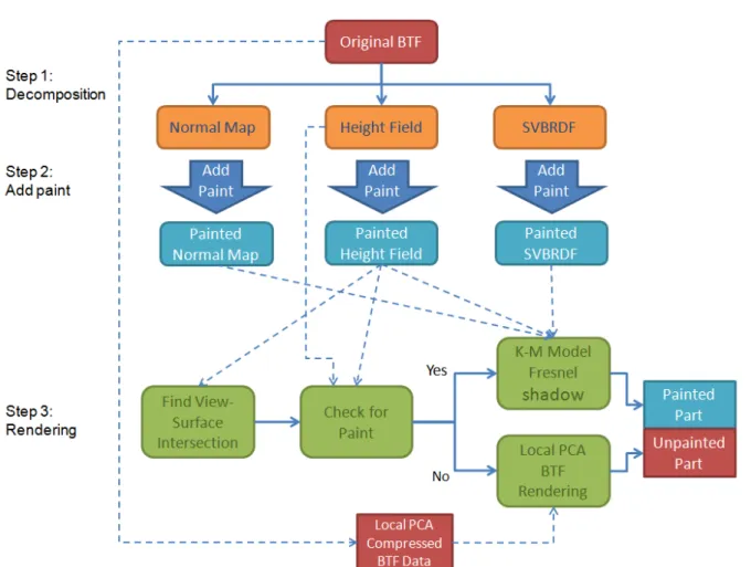
Our method can be roughly divided into three steps. First, we decompose the original BTF into a representation that consists of a height field, a normal map and a corresponding SVBRDF. Next, we apply paint on these three components, i.e., we simulate the changes of these three components caused by paint being applied onto the surface. The height field is changed ev-erywhere according to the thickness of the paint being applied. The normal map is changed according to the changed height field. The SVBRDF is changed according to the reflectance properties and thickness of the applied paint. And eventually, we gather all these modified com-ponents, the painted height field, normal map, and SVBRDF, to produce synthetic images of the painted material. Figure 3.1 is a diagram of this three-step framework.

Whereas representing BTF with a combination of height field and SVBRDF is not a new in-vention in the computer graphics field, we chose this representation because it has the following

3.1 Framework 10

3.2 Height Field and SVBRDF Reconstruction 11 advantages:

1. Height field allows us to simulate the paint flow dynamics

2. SVBRDF combining the Kubelka-Munk model allows us to calculate the painted reflectance of the material

3. The BTF images reproduced by this representation are close to the original BTF images

In the following sections, we first describe how we extract height field, normal map, and SVBRDF from the original BTF. Next, we describe how we modify these components according to the applied paint. In the last section, we describe how we perform rendering with these modified components.

3.2

Height Field and SVBRDF Reconstruction

3.2.1

Height Field and Normal Map Reconstruction

We follow the method used by [MSK07] to reconstruct the height-field and normal map. A photometric stereo technique ([RTG97]) is used to estimate the normal of each texel first and a method using the reconstructed normal information while enforcing surface slope integrability ([FC88]) is used to reconstruct the height-field. To reconstruct normal map and height field from BTF images, some of the methods developed in computer vision can be used directly. As mentioned in [NZG05], there are three types of methods dealing with this kind of problem: mul-tiview, photometric stereo, and Helmholtz stereopsis, depending on the type of data available. In [NZG05] and [MG09], methods that are more suitable for BTF data are also proposed. The reason we’ve chosen [FC88] and [RTG97] is that it has been tested by [MSK07] on BTF data and there exists code implementing the Frankot-Chellappa algorithm [Kov04]. The complete procedure is as follows.

3.2 Height Field and SVBRDF Reconstruction 12 First we select the top view BTF images, i.e. images captured with viewing direction at zero theta degree. Assume there are m top view images. Each texel now has m measurements with known lighting and viewing directions. According to [RTG97], assuming a Lambertian surface illuminated by a distant small source, the reflected radiance Lois given by:

Lo = ρ(Li∆ω/π)(~n · ~l), (3.1)

where ρ is the Lambertian reflectance, Li is the light source radiance, ∆ω is the solid angle

subtended by the light source, ~n is the surface normal and ~l is the direction to the light source. Given the top view BTF measurements, we can form the following matrix equation for the surface normal of each texel:

ρ(Li∆ω/π)         l1,x l1,y l1,z l2,x l2,y l2,z .. . ... ... lm,x lm,y lm,z              nx ny nz      =         Lo,1 Lo,2 .. . Lo,m         (3.2)

This equation allows us to solve for ρ(Li∆ω/π)~n, we then normalize it to get ~n, the normal

vector.

Next, we perform normal integration using the method proposed by Frankot and Chellappa [FC88] to recover the height field. This method obtains the nearest (minimum distance) inte-grable surface slope by projecting the estimated surface slope onto a set of inteinte-grable Fourier basis functions, and the integrability of the recovered height field is enforced using the inte-grable surface slope. This method assumes that the surface we want to recover is a smooth surface, the integrability constraint is therefore used to ensure surface smoothness. The result of this assumption is that it is not suitible to recover surface that has discontinuity. Figure 3.2 shows the recovered normal map and height-field.

3.2 Height Field and SVBRDF Reconstruction 13

Figure 3.2: Original BTF image, reconstructed height field and normal map.

3.2.2

SVBRDF Fitting

Since our goal is to simulate the painted appearance of a BTF material, we need to choose a suitable BRDF model together with a paint model. The BRDF model is used to represent the original material, and the paint model is used to combine the information about the paint, such as type and thickness, with the original material. These two models should work together to calculate the painted appearance of the original material.

The BRDF model that we have chosen is the Lafortune model [LFTG97]. We used a Lafor-tune function consisting of a diffuse term and a single lobe specular term:

fr(ωi, ωo) = ρd+ S(ωi, ωo)

= ρd+ ρs· (Cxωi,xωo,x+ Cy ωi,yωo,y + Czωi,z ωo,z)n,

(3.3) where ωi and ωo are the incident and reflected light directions. The diffuse coefficient ρd and

the specular coefficient ρs are different for each of the RGB channels but the other specular

lobe parameters, i.e. Cx, Cy, Cz, and n are shared by the three channels. Therefore, totally ten parameters are needed for each texel. We first describe how we estimate BRDF parameters for surface that is flat or nearly flat and then for surface that is rough.

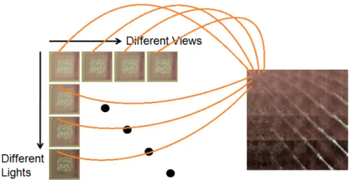
To estimate the SVBRDF for a flat surface, we have adopted the approach proposed in [McA02]. There are roughly five steps for estimating the BRDF parameters for each texel. Before the estimating steps, we gather all the measurements for each texel position from the original BTF images and put them into a single file which we called a measurement file. This

3.2 Height Field and SVBRDF Reconstruction 14

Figure 3.3: Gather all measurements of a texel into a single file.

step is demonstrated in Figure 3.3. The horizontal axis of the measurement file represents different viewing directions while the vertical axis represents different light directions. After gathering all measurements for each texel, we perform BRDF fitting according to the following reflectance equation for a point light source:

Lo(ωo) = fr(ωi, ωo)Li(ωi) cos(θ)∆ωi, (3.4)

where Li(ωi) and Lo(ωo) are the incident and reflected radiance, ∆ωi and θ are the solid angle

and the zenith angle of the incident light. The first step of the fitting process is to remove the irradiance value from each measurement to get the BRDF value, i.e.,

fr(ωi, ωo) =

Lo(ωo)

Li(ωi) cos(θ)∆ωi

. (3.5) After this step, the kth _{measurement value becomes the BRDF value f}(k)

r . Figure 3.4(b) shows

the measurement file after this step. Notice that most of the cosine effect disappeared. The val-ues are rescaled to fit image format. The second step is to find ρd, the diffuse part of the BRDF,

remember that our BRDF model consists of a diffuse term and a specular term according to Equation (3.3). Since the specular part is always positive, theoretically we can use the mini-mum reflectance value as ρd, i.e. ρd = minkf

(k)

3.2 Height Field and SVBRDF Reconstruction 15

(a) (b) (c)

(d) (e) (f)

Figure 3.4: The SVBRDF fitting process. (a) The original measurement file. The horizontal axis represents different viewing directions while the vertical axis represents different light directions. (b) The measurement file after irradiance is removed (rescaled to fit image format). (c) Diffuse part is removed and specular part is left. (d) Specular part is averaged. (e) The fitting result of specular part. (f) The final fitting result. The measurement file is from the WALLPAPER sample of the BTF Database Bonn [SSK03].

3.2 Height Field and SVBRDF Reconstruction 16 light being blocked by neighbouring surface points could lower the minimum value in practice. Thus we used a chosen percentile (10th _{as suggested by [McA02]) as the estimated ρ}

d. After ρd

is determined, the next step is to subtract ρdfrom each BRDF value, leaving only the specular

part. Figure 3.4(c) is the measurement file after subtracting ρd. Since there are three

specu-lar values for the three RGB channels but we want the three channels to share the estimated specular parameters, we take the average of the three values as a single specular value which is to be fitted. Although [McA02] have used a luminance-weighted average, in our experience, the fitting result is better when normal average is used. Figure 3.4(d) shows the measurement file after this average step. The average value is assumed to be the specular part and is then fitted using the Levenberg-Marquardt non-linear optimization algorithm to get the parameters Cx, Cy, Cz, and n. Figure 3.4(e) shows the re-calculated specular part of the BRDF using the estimated Cx, Cy, Cz, and n. Now the only parameter that has not been fitted is ρs. This

parameter is obtained by ρs = 1 m m X k=1 fr,s(k) (Cx ω (k) i,x ω (k) o,x+ Cy ω (k) i,y ω (k) o,y + Cz ω (k) i,z ω (k) o,z)n (3.6) where fr,s(k)is the specular part of fr(k).

For rough surface SVBRDF fitting, we have used a similar method to estimate ρd, and a set

of representative specular parameters estimated from some flat area of the BTF sample are used to represent the whole surface. For each measurement file, we first remove the measurements that are too dark, because these are assumed to be definitely in shadow. After that, we just followed the same procedure as for flat surfaces to remove the cosine effect and then use a chosen percentile as the estimated ρd. For specular parameters, we chose the measurement file

of a representative texel that is in a flat area of the BTF surface. We then estimate specular parameters for this texel using the same procedure for flat surfaces. The estimated specular parameters are then used for the rest of the texels.

3.3 Painting Effects on Height Field and SVBRDF 17

3.3

Painting Effects on Height Field and SVBRDF

After the above steps, we now have the reconstructed geometry and reflectance information about the original BTF sample. In this section, we describe how we modify these components according to the applied paint.

3.3.1

Apply Paints on Height Field and Normal Map

By reconstructing the height field of the original material surface, we are able to use any kind of fluid dynamic simulation algorithm to simulate the flowing of paint on the surface. Since the simulation of paint flow is not our main subject, we have only adjusted the height field by hand. Nonetheless, we believe that if a fluid dynamic simulation algorithm such as [BWL04] or [CT05] has been used, the final rendering result would be better. The normal map is recalculated using the modified height field.

3.3.2

The Paint Model

The paint model that we have chosen is the Kubelka-Munk model [Kor69]. The Kubelka-Munk model is derived from a more general equation which is called the radiation transfer equation. Rather than concerning the individual behaviour of each pigment particle, the radiation transfer equation describes radiation transfer in a medium by some descriptive coefficients, such as the absorption coefficient, the scattering coefficient, and the scattering phase function, regarded as characteristic properties of the whole medium. The first attempt to obtain a simplified solution to the equation was made by Schuster. His method consists of simplifying the problem to plane parallel layers, assuming isotropic scattering, and simplifying the radiation field into two oppositely directed radiation fluxes I and J in the x and −x directions respectively. Also, the extension of the layer in the yz-plane is assumed to be great compared with the thickness of the layer, so that edge effects may be ignored. Figure 3.5 shows this simplified condition within a layer. Kubelka and Munk further assumes that the particles in the layer are randomly distributed

3.3 Painting Effects on Height Field and SVBRDF 18 and their sizes are much smaller than the thickness of the layer itself. The layer is subject only to diffuse irradiation. With the above assumptions, Kubelka and Munk came out the equations that can be used to calculate the reflectance and transmittance of a layered surface. The book by Kortum provides more details about the Kubelka-Munk theory[Kor69].

The K-M model describes the reflectance and transmittance of a paint layer by the scattering coefficient S and the absorption coefficient K of the paint. These coefficients are functions of wavelength, thus we have to specify different values for individual RGB channels. Given the scattering coefficient S and the absorption coefficient K of a paint layer of thickness d, the K-M model allows us to compute the reflectance R and the transmittance T of the layer:

R = sinh bSd c T = b

c

(3.7) where a = (S + K)/S, b =√a2_{− 1, and c = a sinh bSd + b cosh bSd.}

For two overlapping layers, the following equations allow us to determine the overall re-flectance and transmittance of the composite layer:

R = R1+ T2 1R2 1 − R1R2 T = T1T2 1 − R1R2 (3.8) where R1and T1are the reflectance and transmittance of the upper layer, R2and T2are those of

the lower layer, and R and T are those of the composite layer. For a stack of layers, we can just

3.3 Painting Effects on Height Field and SVBRDF 19 repeat this compositing process for each layer from button to top to get the overall reflectance and transmittance.

3.3.3

Apply Paints on SVBRDF

The method that we use to modify the material SVBRDF can be separated into two parts, the diffuse part and the specular part. For the diffuse part, we use the K-M model to modify the original material ρd to produce the new painted diffuse term ρmd. First, we need to choose a

paint type, i.e., the S and K values of the paint, and the paint layer thickness d. The thicker the paint layer is, the more the color of the underlying surface is covered by the paint color. Next, we compute the reflectance Rpl and transmittance Tpl of the paint layer using Equation (3.7)

with the S and K of the chosen paint type and the thickness d of the paint layer. After that, we use Equation (3.8) with Rpl and Tpl as R1 and T1 and ρdof the BTF material as R2 to compute

the new painted diffuse ρm_d :

ρm_d = Rpl+

T2 plρd

1 − Rplρd

. (3.9) If there are more than one paint layer, we could repeat this procedure for each paint layer from the bottom to top to compute the composite reflectance. The S and K coefficients that we used for our experiments come from two sources, one is the oil paint data from [BWL04] and the other is the watercolor data from [CAS+97]. Although [BWL04] provides us the 101-wavelength data which is more accurate than standard RGB model, limited to the RGB form of the original BTF data, we have only sampled RGB wavelength from the 101-wavelength data. The three wavelenghs for RGB that we sampled are 652 nm, 532 nm, and 460 nm. While [BWL04] also proposed to use Gaussian quadrature to reduce the 101-wavelength data to 8-wavelength according to the light source spectrum, the 8-wavelengths are automatically decided such that we can not restrict Gaussian quadrature to choose RGB channels, besides we don’t know the light source spectrum of the BTF data. On the other hand, the watercolor data from [CAS+_{97] follows the RGB model so that we could use it directly as test data. By specifying the}

3.4 Rendering 20 the S and K values by reversing the K-M equations. Fig. 3.6 shows these S and K values.

For the specular part, since K-M model can not handle the specular term S(ωi , ωo) of the

original material, and considering this term into our lighting computation would be too complex for our application, we have decided to drop it and add a new specular term calculated using Fresnel equation. For BTF materials that are closer to diffuse reflection, the influence would be small, but for BTF materials that are closer to specular reflection, dropping the original spec-ular term might darken the final painted result. The specspec-ular reflection of light is motivated from light reaching an interface between two materials of different refractive indices which in our case are the air and the paint. This phenomenon is quantitatively described by the Fresnel equation, so we use it to calculate the new specular effect. We have used Schlick’s Fresnel approximation in our implementation. Since we don’t have actual measurement values of re-fractive indices of paints, these are set to around 1.5 ∼ 2.0. Some sample values of rere-fractive indices of different binding media and pigments could be found in [Bud07].

3.4

Rendering

We have implemented our rendering algorithm using graphics hardware. Although we could render a BTF-mapped object with a paint pattern on it without using the original BTF data, i.e. using the reconstructed and painted height-fields, the normal map, and the SVBRDF, we think that this would lose some complexity hidden in the original BTF data. Thus we have integrated a BTF rendering algorithm, i.e. the local PCA method[MMK03b], into our rendering system to compensate the lost information during the height field reconstruction and SVBRDF fitting processes. The local PCA method rearrange the BTF data into a BRDF-wise arrangement first, and then perform clustering and principle component analysis(PCA) iteratively to compress the data. The compressed data would be a cluster map, a PCA weights map, and the eigen vectors for each cluster. These are stored as 2D or 3D textures for use in the rendering process. We integrated this method to render the unpainted part of the object surface.

ray-3.4 Rendering 21

3.4 Rendering 22 tracing algorithm such as [POC05] to find the view-surface intersection point. By comparing the painted height-field value and the original height-field (i.e. the height field recovered from the original BTF) value at that surface point, we can know if this point is a painted point or an unpainted point (The painted and original height-fields are all stored in texture memory). If it is an unpainted point, we use the local PCA method to approximate the original BTF. If it is a painted point, the Kubelka-Munk model is used to calculate the painted reflectance, and a Fresnel specular term is added. To produce results closer to real situation, we have also adapted the parallax occlusion mapping(POM,[Tat06]) technique to simulate self-shadowing effect for the painted part. The above steps are all performed in the fragment shader. The lower half of Fig. 3.1 shows this rendering workflow.

When using the local PCA method for BTF rendering, we need to take multiple texture samples for each pixel, otherwise the rendering result would be blocky because of texture mag-nification. We have compared the results of taking 5 samples, 9 samples and 25 samples for each pixel, and found that the results are almost the same but the rendering speeds are very different, that is roughly linear to the number of samples, thus we took only 5 samples in our final implementation.

C H A P T E R

4

Results

We have tested our method on several BTF materials. All our programs run on an Intel Core 2 Duo 3.0GHz CPU. We use Matlab to perform photometric stereo normal estimation and Frankot-Chellappa height-field reconstruction. The time needed for these two steps is negli-gible. For the SVBRDF fitting, the most time-consuming step is performing the Levenberg-Marquardt non-linear optimization. It takes around 10 seconds to perform this step for each texel on Matlab, therefore several hours are needed even for a 64 × 64 BTF sample. Thus we have implemented another C++ version fitting program that takes only a few minutes to finish the fitting process for the same BTF sample.

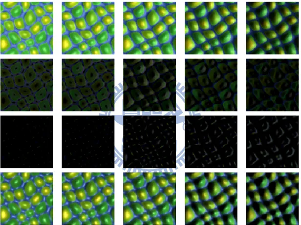
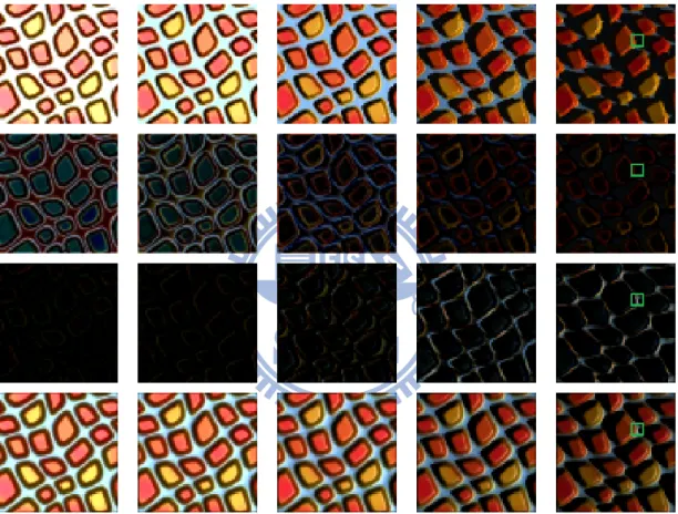
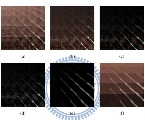
A comparison between the original BTF images and images rendered with reconstructed information are shown in Figure 4.1 and 4.2. The upper rows are the original BTF images and the bottom rows are the reconstructed images. The second rows are the positive part of the original images subtract the reconstructed images and the third rows are the negative part. As can be seen from the figures, the original surface shape and the reconstructed surface shape are a little bit different. In Figure 4.2, the edge of each block seems to be smoother than original. This might be the result of using the Frankot-Chellappa algorithm because its preserving integrability

24 nature tends to smooth the reconstructed result. Also, the reconstructed images are darker than the original ones especially for images of lower zenith angles. The reason for this might be inaccuracy in diffuse estimation. For the images of higher zenith angles, errors caused by shadows and specular effects are more noticable. As can be seen from the green boxes in each image of the last column in Figure 4.2, the area in the original image is under shadow while the same area is not under shadow in the reconstructed image. Despite these errors, the reconstructed images still preserve the look and feel of the original BTF images.

After the SVBRDF fitting process, we can use the K-M model to produce the painted BTF images. Figure 4.3 and Figure 4.4 show the results of adding different kinds of paints onto the hole BTF sample. The thickness of the paint in each image is the same everywhere. The shadows are rendered with parallax occlusion mapping [Tat06]. We have also compared the rendered results with alpha blending since alpha blending is an intuitive way to change surface color. Figure 4.5 and Figure 4.6 show these comparisons. The first row in each block shows the painted BTF images with the same viewing and lighting angles but different paint thicknesses. The second row shows the alpha blending results with alpha 0.25, 0.5, 0.75, and 1. Apparently alpha blending is not a good method for changing the surface color, unless the material is flat.

Next, we show the results of adding paint patterns on 3D models. To render the painted part of the model, we use only the reconstructed information to represent the original material, i.e. the reconstructed height-field, the reconstructed normal map, and the SVBRDF, and the reflectance is calculated using K-M model and Fresnel equation with the paint parameters. To render the unpainted part of the model, we could still use only the reconstructed information of the material. However, as described previously, we have combined the local PCA method to render the unpainted part of the model to fully exploit the complexity of the original BTF. Before using the local PCA BTF rendering method [MMK03a], the original BTF data need to be compressed. The local PCA compression is another task that needs quite a long time to execute. It depends on the BTF data size and the required compression quality. In our experience, performing 10 iterations for a 64 × 64 BTF data with 51 × 51 view-light pairs takes about 100 minutes. After the compression, the compressed data can be used for rendering.

25

Figure 4.1: Comparison between original BTF images and fitting results. The images are all top-view images and the lights are all from the right side with theta 0, 17, 30, 50, and 65 degrees.

26

Figure 4.2: Another comparison between original BTF images and fitting results. The images are all top-view images and the lights are all from the right side with theta 0, 17, 32, 50, and 65 degrees.

27

Figure 4.3: The top row shows the original BTF images of the hole sample. The second to the last rows are results of painting the hole surface with three different kinds of watercolor paints: Quinacridone Rose(thicknesses 0.2 and 0.4), Cerulean Blue(thicknesses 0.2 and 0.4), and Cadmium Yellow(thicknesses 0.2 and 0.3).

28

Figure 4.4: The top row shows the original BTF images of the hole sample. The second to the last rows are results of painting the hole surface with three different kinds of oil paints: Alizarin Crimson(thicknesses 0.04 and 0.2), Sap Green(thicknesses 0.1 and 0.4), and Cadmium Yellow(thicknesses 0.04 and 0.08).

29

Figure 4.5: Painted BTF v.s. alpha blending. The leftmost images are the original BTF images. The first row in each block shows the painted BTF images with the same viewing and lighting angles but with different paint thicknesses. The second row shows the alpha blending results with alpha 0.25, 0.5, 0.75, and 1. The paints used in these images are water color Cadmium Red, French Ultramarine, and Cadmium Yellow from top to bottom.

30

Figure 4.6: Painted BTF v.s. alpha blending. The leftmost images are the original BTF im-ages. The first row in each block shows the painted BTF images with the same viewing and lighting angles but with different paint thicknesses. The second row shows the alpha blending results with alpha 0.25, 0.5, 0.75, and 1. The paints used in these images are oil paints Alizarin Crimson, Cobalt Blue, and Cadmium Yellow from top to bottom.

31 Figure 4.7 and Figure 4.8 show comparisons between renderings using local PCA and using only the reconstructed information for the unpainted part of the model. Notice that although we have used two different rendering methods for the painted part and the unpainted part, the result does not show distinguishable inconsistency. Also, the splash paint pattern looks more realistic than evenly applied paint layer.

Figure 4.9 and Figure 4.10 show the rendering results of another BTF sample on a lizard model with different watercolor and oil paints. Comparing these two images, we can see that images using watercolor and images using oil paint seem to be different only on the colors. This is because we’ve only changed the K and S coefficients. In order to exhibit more different characteristics between watercolor and oil paint, we also need to consider the flowing pattern caused by different viscosities and the different interactions between paints and surfaces.

In Figure 4.11 and Figure 4.12, results using different refractive indices are demonstrated. Different refractive indices can be used to simulate wet or dry paints. Notice that different background colors causing different painted appearances. We have chosen a neat purplish red flower pattern which is similar to the pattern of the original BTF material making the paints look more like dyes.

Figure 4.13 and Figure 4.14 show rendering results using a paint brush pattern demonstrat-ing how our method can express the thickness of the paint. A viewer determine how thick the paint is by clues from both geometry and reflectance information. In our framework, the geometrical clue is produced by the painted height field, displacement mapping, and shadow; the reflectance clue is controlled by the thickness parameter d of the K-M model. For larger d, the painted result is less influenced by the underlying surface color, revealing a purer color from the paint. Combining these two kinds of clues, a viewer can perceive the thickness of the paint. To produce accurate thickness effect, the paint thickness from the painted height field should be consistent to the K-M model input d. Since height field is stored as general image format, i.e. each height value or paint thickness is stored as 0 − 255 on a height field image, this value should be transformed into K-M model thickness parameter d during rendering stage in the fragment shader. We have not yet find a good way to define how thick in reality the paint

32

(a)

(b)

Figure 4.7: A comparison between renderings (a) using local PCA and (b) using only the re-constructed information. The paint is watercolor Cadmium Yellow.

33

(a)

(b)

Figure 4.8: A comparison between renderings (a) using local PCA and (b) using only the re-constructed information. The paint is oil paint Cadmium Yellow.

34 thickness on the height field represent, since we don’t know how thick the original BTF surface is either. In other word, since we don’t know how thick a 1 on height field represent in reality, we can not define how thick a paint thickness value on height field represent in reality. For now, we just use a scaling factor to transform this value into d. In Figure 4.13 and Figure 4.14, the paint thickness in the second image is twice the paint thickness in the first image, and the paint thickness in the third image is trice that in the first image.

Figure 4.15 and Figure 4.16 show examples of multiple paint layers which are combined together using Equation (3.8). The graphics cards we used for our experiments are Nvidia GeForce 9600GT and GTS250. The rendering fps for a 768 × 768 window size is around 10 to 30.

35

Figure 4.9: A splash pattern with different watercolor paints on a lizard model. The paints are Burnt Umber, Quinacridone Rose, and Cadmium Red from top to bottom. The refractive indices are all set to 1.8.

36

Figure 4.10: A splash pattern with different oil paints on a lizard model. The paints are Prussian Blue, Alizarin Crimson, and Titanium White from top to bottom. The refractive indices are all set to 1.8.

37

Figure 4.11: A flower pattern with different refractive indices on a cloth model. The refractive indices are set to 1.8, 2.0, and 2.2 from top to bottom. The paint is watercolor Quinacridone Rose.

38

Figure 4.12: A flower pattern with different refractive indices on a cloth model. The refractive indices are set to 1.8, 2.0, and 2.2 from top to bottom. The paint is oil paint Alizarin Crimson.

39

Figure 4.13: Results of a paint brush pattern. The paint type is watercolor Burnt Umber. The paint thickness in the second image is twice the paint thickness in the first image, and the paint thickness in the third image is trice that in the first image.

40

Figure 4.14: Results of a paint brush pattern. The paint type is oil paint Burnt Sienna from [BWL04]. The paint thickness in the second image is twice the paint thickness in the first image, and the paint thickness in the third image is trice that in the first image.

41

Figure 4.15: An example of using four paint layers. The four images in the bottom row are the scaled paint pattern images. The paints used for four paint patterns from left to right are watercolors: French Ultramarine, Quinacridone Rose, Brilliant Orange, and Phthalo Green.

42

Figure 4.16: An example of using four paint layers. The four images in the bottom row are the scaled paint pattern images. The paints used for four paint patterns from left to right are oil paints: Cobalt Blue, Alizarin Crimson, Burnt Sienna, and Viridian.

C H A P T E R

5

Conclusion

In order to further use the BTF data that are not very easy to acquire, we have proposed the problem of how to simulate the painted appearance of a BTF material in this thesis, and we have developed a simple yet effective method to solve this problem. The method first try to recover neccesary information from the original BTF data, including both geometry and reflectance information, and then use these recovered information and the original data to produce the illusion of a painted surface. Our rendering framework have integrated the local PCA BTF rendering method in order not to waste any information hidden in the raw BTF data. The method is simple and intuitive, yet the results are novel.

Nonetheless, there are still rooms for improvements in each solution step. Here we list some of them. First of all, to simulate the changed appearance of the painted material, we have chosen the Lafortune BRDF model and the Kubelka-Munk reflectance model. Since BTF can be used to represent any kind of materials, the Lafortune model might not suitable for all of them. Is there other suitable BRDF model for this application? If we use other BRDF model, will it be compatible with the K-M model? Also, since there are lots of simplifying assumptions for the K-M model which make the model simple but sometimes not conform to the real conditions,

44 how to break these assumptions so that the model can fit into more complex situations? Or is there a better reflectance model for our application? Besides the BRDF and reflectance model, we would like to implement some paint flow simulation algorithm since we didn’t implement one in this work, and we would like to investigate the physical reaction happened when paint is applied to a substrate. This physical process is much more complicated then what we have considered in this thesis. Different paints can have different physical properties, and different substrates can have different responses to the same paint. Some effect such as the capillarity effect is what we have missed in our simulation. To more accurately calculate the reflectance of the painted material, we should know all these detail information. Besides, there have been research considering these effects [LAD08].

Lastly, we would like to extend our work to simulate the aging and weather phenomenon such as stains, pollution, mold, steal rusting and patinas.

Bibliography

[BGM06] Jeffrey B. Budsberg, Donald P. Greenberg, and Stephen R. Marschner. Re-flectance measurements of pigmented colorants. 2006.

[Bud07] Jeffrey B. Budsberg. Pigmented colorants: Dependence on media and time. Mas-ter’s thesis, 2007.

[BWL04] William Baxter, Jeremy Wendt, and Ming C. Lin. Impasto: a realistic, interactive model for paint. In NPAR ’04: Proceedings of the 3rd international symposium on Non-photorealistic animation and rendering, pages 45–148, New York, NY, USA, 2004. ACM.

[CAS+97] Cassidy J. Curtis, Sean E. Anderson, Joshua E. Seims, Kurt W. Fleischer, and David H. Salesin. Computer-generated watercolor. In SIGGRAPH ’97: Proceed-ings of the 24th annual conference on Computer graphics and interactive tech-niques, pages 421–430, New York, NY, USA, 1997. ACM Press/Addison-Wesley Publishing Co.

[CCCC08] Ying-Chieh Chen, Sin-Jhen Chiu, Hsiang-Ting Chen, and Chun-Fa Chang. Physically-based analysis and rendering of bidirectional texture functions data. Journal of Information Science and Engineering, 24(1), 2008.

[CT05] Nelson S.-H. Chu and Chiew-Lan Tai. Moxi: real-time ink dispersion in ab-sorbent paper. ACM Trans. Graph., 24:504–511, July 2005.

Bibliography 46 [DH96] Julie Dorsey and Pat Hanrahan. Modeling and rendering of metallic patinas. In SIGGRAPH ’96: Proceedings of the 23rd annual conference on Computer graphics and interactive techniques, pages 387–396, New York, NY, USA, 1996. ACM.

[DVGNK99] K.J. Dana, B. Van-Ginneken, S.K. Nayar, and J.J. Koenderink. Reflectance and Texture of Real World Surfaces. ACM Transactions on Graphics (TOG), 18(1):1– 34, Jan 1999.

[FC88] Robert T. Frankot and Rama Chellappa. A method for enforcing integrability in shape from shading algorithms. IEEE Trans. Pattern Anal. Mach. Intell., 10(4):439–451, 1988.

[FH04] Jiri Filip and Michal Haindl. Non-linear reflectance model for bidirectional tex-ture function synthesis. In ICPR ’04: Proceedings of the Pattern Recognition, 17th International Conference on (ICPR’04) Volume 1, pages 80–83, Washing-ton, DC, USA, 2004. IEEE Computer Society.

[FH05] J. Filip and M. Haindl. Efficient image based bidirectional texture function model. In M. Chantler and O. Drbohlav, editors, Texture 2005: Proceedings of 4th Internatinal Workshop on Texture Analysis and Synthesis, pages 7–12, Ed-inburgh, October 2005. Heriot-Watt University.

[FH09] Jiri Filip and Michal Haindl. Bidirectional texture function modeling: A state of the art survey. IEEE Transactions on Pattern Analysis and Machine Intelligence, 31:1921–1940, 2009.

[GTR+06] Jinwei Gu, Chien-I Tu, Ravi Ramamoorthi, Peter Belhumeur, Wojciech Matusik, and Shree Nayar. Time-varying surface appearance: acquisition, modeling and rendering. In SIGGRAPH ’06: ACM SIGGRAPH 2006 Papers, pages 762–771, New York, NY, USA, 2006. ACM.

Bibliography 47 [HF03] M. Haindl and J. Filip. Fast BTF texture modelling. In M. Chantler, editor, Texture 2003. Proceedings, pages 47–52, Edinburgh, October 2003. IEEE Press. [HF04] Michal Haindl and Jiri Filip. A fast probabilistic bidirectional texture function model. In Aurelio Campilho and Mohamed Kamel, editors, Image Analysis and Recognition, volume 3212 of Lecture Notes in Computer Science, pages 298– 305. Springer Berlin / Heidelberg, 2004.

[HF07] Michal Haindl and Jiri Filip. Extreme compression and modeling of bidirectional texture function. IEEE Trans. Pattern Anal. Mach. Intell., 29(10):1859–1865, 2007.

[HFA04] Michal Haindl, Jiri Filip, and Michael Arnold. Btf image space utmost compres-sion and modelling method. In ICPR ’04: Proceedings of the Pattern Recog-nition, 17th International Conference on (ICPR’04) Volume 3, pages 194–197, Washington, DC, USA, 2004. IEEE Computer Society.

[KBD07] Jan Kautz, Solomon Boulos, and Fr´edo Durand. Interactive editing and modeling of bidirectional texture functions. ACM Trans. Graph., 26(3):53, 2007.

[KMBK03] Melissa L. Koudelka, Sebastian Magda, Peter N. Belhumeur, and David J. Krieg-man. Acquisition, compression, and synthesis of bidirectional texture functions. In In ICCV 03 Workshop on Texture Analysis and Synthesis, 2003.

[Kor69] Gustav Kort¨um. Reflectance Spectroscopy (Principles, Methods, Applications). Springer-Verlag New York Inc., 1969.

[Kov04] Peter Kovesi. An implementation of frankot and chellappa algorithm, 2004. [LAD08] Toon Lenaerts, Bart Adams, and Philip Dutr´e. Porous flow in particle-based fluid

simulations. In SIGGRAPH ’08: ACM SIGGRAPH 2008 papers, pages 1–8, New York, NY, USA, 2008. ACM.

Bibliography 48 [LFTG97] Eric P. F. Lafortune, Sing-Choong Foo, Kenneth E. Torrance, and Donald P. Greenberg. Non-linear approximation of reflectance functions. In SIGGRAPH ’97: Proceedings of the 24th annual conference on Computer graphics and interactive techniques, pages 117–126, New York, NY, USA, 1997. ACM Press/Addison-Wesley Publishing Co.

[LH06] Sylvain Lefebvre and Hugues Hoppe. Appearance-space texture synthesis. In SIGGRAPH ’06: ACM SIGGRAPH 2006 Papers, pages 541–548, New York, NY, USA, 2006. ACM.

[McA02] David Kirk McAllister. A generalized surface appearance representation for computer graphics. PhD thesis, 2002. Director-Lastra, Anselmo.

[MCC+04] Wan-Chun Ma, Sung-Hsiang Chao, Bing-Yu Chen, Chun-Fa Chang, Ming Ouhy-oung, and Tomoyuki Nishita. An efficient representation of complex materials for real-time rendering. In VRST ’04: Proceedings of the ACM symposium on Vir-tual reality software and technology, pages 150–153, New York, NY, USA, 2004. ACM.

[MCT+_{05] Wan-Chun Ma, Sung-Hsiang Chao, Yu-Ting Tseng, Yung-Yu Chuang, Chun-Fa}

Chang, Bing-Yu Chen, and Ming Ouhyoung. Level-of-detail representation of bidirectional texture functions for real-time rendering. In I3D ’05: Proceedings of the 2005 symposium on Interactive 3D graphics and games, pages 187–194, New York, NY, USA, 2005. ACM.

[MG09] Nicolas Menzel and Michael Guthe. g-brdfs: An intuitive and editable btf repre-sentation. Comput. Graph. Forum, 28(8):2189–2200, 2009.

[MMK03a] Jan Meseth, Gero M¨uller, and Reinhard Klein. Preserving realism in real-time rendering of bidirectional texture functions. In OpenSG Symposium 2003, pages 89–96. Eurographics Association, Switzerland, April 2003.

Bibliography 49 [MMK03b] Gero M¨uller, Jan Meseth, and Reinhard Klein. Compression and real-time ren-dering of measured btfs using local pca. In T. Ertl, B. Girod, G. Greiner, H. Nie-mann, H.-P. Seidel, E. Steinbach, and R. WesterNie-mann, editors, Vision, Modeling and Visualisation 2003, pages 271–280. Akademische Verlagsgesellschaft Aka GmbH, Berlin, November 2003.

[MMK04] Jan Meseth, Gero M¨uller, and Reinhard Klein. Reflectance field based real-time, high-quality rendering of bidirectional texture functions. Computers and Graph-ics, 28(1):103–112, February 2004.

[MMS+04] Gero M¨uller, Jan Meseth, Mirko Sattler, Ralf Sarlette, and Reinhard Klein. Acquisition, synthesis and rendering of bidirectional texture functions. In Christophe Schlick and Werner Purgathofer, editors, Eurographics 2004, State of the Art Reports, pages 69–94. INRIA and Eurographics Association, Septem-ber 2004.

[MSK07] Gero M¨uller, Ralf Sarlette, and Reinhard Klein. Procedural editing of bidirec-tional texture functions. In J. Kautz and S. Pattanaik, editors, Eurographics Sym-posium on Rendering 2007. The Eurographics Association, June 2007.

[NZG05] A. Neubeck, A. Zalesny, and L. Van Gool. 3d texture reconstruction from exten-sive btf data. In Texture 2005 Workshop in conjunction with ICCV 2005, pages 13–19, October 2005.

[ON05] Crystal S. Oh and Yang-Hee Nam. Gpu-based 3d oriental color-ink rendering. In Proceedings of the 2005 international conference on Augmented tele-existence, ICAT’05, pages 142–147, New York, NY, USA, 2005. ACM.

[POC05] F´abio Policarpo, Manuel M. Oliveira, and ao L. D. Comba, Jo˙ Real-time relief mapping on arbitrary polygonal surfaces. ACM Trans. Graph., 24(3):935–935, 2005.

Bibliography 50 [RMN03] Dave Rudolf, David Mould, and Eric Neufeld. Simulating wax crayons. In PG ’03: Proceedings of the 11th Pacific Conference on Computer Graphics and Ap-plications, page 163, Washington, DC, USA, 2003. IEEE Computer Society. [RTG97] Holly E. Rushmeier, Gabriel Taubin, and Andr´e Gu´eziec. Applying shape from

lighting variation to bump map capture. In Proceedings of the Eurograph-ics Workshop on Rendering Techniques ’97, pages 35–44, London, UK, 1997. Springer-Verlag.

[SBLD03] Frank Suykens, Karl Vom Berge, Ares Lagae, and Philip Dutre. Interactive ren-dering with bidirectional texture functions. Computer Graphics Forum, 22:463– 472, 2003.

[SSK03] Mirko Sattler, Ralf Sarlette, and Reinhard Klein. Efficient and realistic visualiza-tion of cloth. In EGRW ’03: Proceedings of the 14th Eurographics workshop on Rendering, pages 167–177, Aire-la-Ville, Switzerland, Switzerland, 2003. Euro-graphics Association.

[Tat06] Natalya Tatarchuk. Dynamic parallax occlusion mapping with approximate soft shadows. In I3D ’06: Proceedings of the 2006 symposium on Interactive 3D graphics and games, pages 63–69, New York, NY, USA, 2006. ACM.

[VT04] M. Alex O. Vasilescu and Demetri Terzopoulos. Tensortextures: multilinear image-based rendering. ACM Trans. Graph., 23(3):336–342, 2004.

[WWS+_{05] Hongcheng Wang, Qing Wu, Lin Shi, Yizhou Yu, and Narendra Ahuja.}

Out-of-core tensor approximation of multi-dimensional matrices of visual data. ACM Trans. Graph., 24(3):527–535, 2005.

[XTJ+07] Songhua Xu, Haisheng Tan, Xiantao Jiao, Francis C.M. Lau, and Yunhe Pan. A generic pigment model for digital painting. Computer Graphics Forum, 26(3):609–618, 2007.