邊界頻譜法在勢流場的應用(I)

行政院國家科學委員會專題研究計畫成果報告

邊界頻譜法在勢流場的應用

Boundar y spectr al method for potential flows

計畫編號：NSC 88-2611-E-002-006

執行期限：88 年 8 月 1 日至 89 年 7 月 31 日

主持人：黃維信 國立台灣大學造船及海洋工程學系

一、中文摘要 傳統上，積分方程式在計算方法上﹐最 常用的技巧是邊界元素法﹐目前常用的元素 是由二次或更低階的多項式構建而成﹐一般 將二次多項式所構建的元素即稱為高階邊界 元素法。有鑒於一般的邊界元素對於包含高 過二階的多項式有奇異點(singularities)的積 分造成的困難﹐以往的學者使用座標轉換或 適應積分(adaptive integration)﹐求解此奇異 點的積分，但這種作法往往會降低邊界元素 法的靈活度及精確度。本計畫主持人提出另 一類技巧﹐以解析的方式將奇異點的積分轉 換為一般的積分﹐因此在數值計算上有重大 進展，可以處理任意階多項式的積分奇異。 邊界積分法最大好處能將一般三維問 題縮減成二維的問題來計算﹐因此在本計畫 中﹐預計發展一種全新的元素“邊界頻譜元素 “來克服一般邊界元素法階數的限制，降低數 值計算所需的容量。進而增加運算速度，並 提高準確度。 關鍵詞：勢流理論、頻譜法、非奇異積分方 程 Abstr act

A boundary spectral method is developed for solving three-dimensional exterior potential problems. This method directly applies spectral approximations and numerical integration such

as Gaussian quadrature or trapezoidal rules successfully. The singularities of the integral equations are completely removed by the Gauss flux theorem and the equipotential theorem. Therefore, all the integrals are non-singular and can be executed accurately and efficiently. By spectral approximation, the unknown variable is expressed as a truncated series of basis functions, which are orthogonal usually. Instead of solving the variables at collocation points in the conventional methods, only the coefficients of basis functions are determined in the present approach. It is shown that the new method reduces a lot of number of unknowns, storage of matrix elements, and computer time for solving the algebraic equations.

Keywor ds: boundary integral equation;

spectral method; potential flows

二、緣由與目的

In the last three decades, the boundary element method (BEM) has become very popular and has been applied to solve a wide range of engineering problems. Since the BEM frequently uses local elements, their basis functions are usually low-order polynomials. In the present paper, a spectral approach is proposed to solve boundary integral equations and it is quite different from traditional BEMs.

For potential flows, since Hess and Smith published their famous work on the BEMs (or called panel methods), a large progress has

been reached. [1] Most of the original BEMs, developed to solve the strength of singularities such as source, vortex, or doublet, are called indirect methods. Later, a Green's formula based method was developed in which the primary unknown was the velocity potential. [2] Both methods are still popularly used currently, but only the direct method is adopted in the present paper.

The spectral method has also been developed for decades and very successful in solving partial differential equations when very high accuracy is needed. It is well known that a truncated Fourier series can approximate any function and its rate of convergence of such a series depends on the smoothness of function itself. Until recently, spectral methods have not been widely used in solving boundary integral equations.

The difficulty of combining the spectral method and the boundary integral equation is due to the singular integrals in the boundary integral equation. There are several methods in the literature to calculate singular integrals such as polar transformations, adaptive sub-division scheme and etc. However, those methods are inefficient when compared with regular integration. In order to avoid such singular integrals, in the present paper we use the subtracting and adding-back technique to evaluate singular integrals. By this scheme, the singularities of the integral kernels can be regularized, and the resultant integrand in the modified Green's formula is bounded. [3] The bounded integrands are excellent for numerical quadrature. The numerical formulation can yield very accurate solutions with significantly fewer terms by most numerical quadrature method.

In the literature, some authors already tried to develop the boundary spectral method. Some of them use analytic formulas to solve two-dimensional cases, and call it boundary strip methods or boundary spectral strip methods. [4,5] But in general their method cannot be extended into three-dimensional

already developed a method to handle three-dimensional smooth bodies for exterior flow field. [6,7] This method can directly be applied in the two-dimensional cases without any difficulty. In this paper, we discuss the detailed variation for the uniform flows past different spheroids, and try to understand the limitation of boundary spectral methods.

三、結果與討論

　For simplicity, in the following three axisymmetrical cases are presented. Since the flow is axisymmetric, we can choose one-dimensional basis functions and the Chebyshev polynomial, Tn(x), is used. The first numerical

example is for the scattering problem of a uniform flow past a sphere. The velocity potential for a uniform flow of magnitude U approaching a sphere of radius a, centered at origin, along positive x axis can be expressed as

Φ( , )R U R( a ) cos R

θ = + 3₂ θ

2 (1)

where θ is the angle between the x-axis and the position vector, and R the distance to the origin. The velocity potential on the sphere surface is

Φ(a, θ) = 3Ux/2 when R = a. In Table 1, a 15-point Gauss-Legendre formula is applied in the x direction and trapezoidal rules is used in the

θ direction. The first 6 terms of Chebyshev polynomials are calculated, and the maximum error, which occurs at two ends x=±1, is less than 10-4.

The second example is the problem of a uniform flow past a prolate spheroid. The prolate spheroid is an elongated ellipsoid of revolution with major axis of length a on the x-axis and minor x-axis of length b. The uniform flow of magnitude U travels along the positive x-axis. The exact solution derived in Milne-Thomson is Φ = αUx, where α depends on a and b. Again, Chebyshev polynomials, the 15-point Gauss-Legendre formula in the x

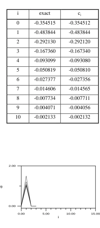
direction are applied. Table 2 shows the values of coefficient c1 for different slenderness of

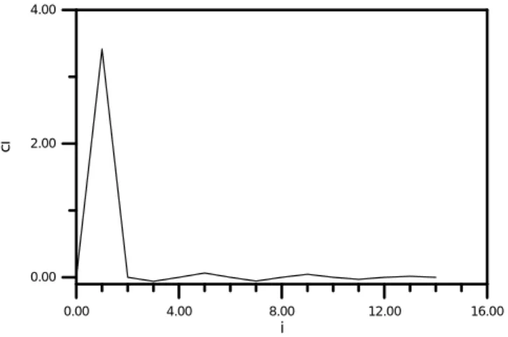
spheroids. For elongate spheroid these main coefficients are very accurate. The other terms are negligible as shown in Fig. 1. For oblate spheroid, the accuracy becomes less and less when b/a becomes larger. Part of the reason is the variation of velocity potential becomes larger. In the case b/a=4, the relative error of c1

is about 1%. In Fig. 2, we show the trend of coefficients for the case b/a=4.

The third example is the problem for a sphere in a doublet flow. A doublet of strength

µ locates at (l, 0, 0) along the positive x

direction outside a sphere, centered at the origin, with radius a (a < l). The flow field is

constructed by the doublet of strength µ at (l, 0,

0) and a doublet with strength -µa3

/l3

at its image point (a2/l, 0, 0). The corresponding

velocity potential on the sphere surface is

Φ( , ) ( ) / a l a l a l lx θ µ π = − + − 4 ₂ 2 2 2 2 3 2 (2)

In this case, 25 Gaussian points and 15 terms of Chebyshev polynomials are used for the example l/a = 2 and 4πa2

/µ=1. The comparison of exact and numerical coefficients of Chebyshev polynomials is greatly consistent. Only first 10 terms are shown in Table 3, while 15 terms are calculated actually. The maximum deviation of coefficients is 0.00004. When i > 3, the ratio between two consecutive terms is approximately half. It indicates the coefficient sequence has exponential convergence. The non-dimensional velocity potential versus to x is plotted in Fig. 3. The maximum error at the calculated points is about 0.01%. This error is of the same order as 25-point formulation by the direct method without the spectral series. It confirms that the reduction of the matrix size does not affect the accuracy significantly. Since the size of matrix A is small, the memory space, and computing time for forming and solving matrix A are also saved lots of amount.

四、參考文獻

[1] J. L. Hess and A. M. O. Smith, 'Calculation of nonlifting potential flow about arbitrary three-dimensional bodies,' J. Ship Research, 8, (1964). [2] L. Morino and C.C. Kuo, 'Subsonic potential

aerodynamics for complex configurations: a general theory,' AIAA J., 12, 191-197 (1974). [3] W.S. Hwang and Y.Y. Huang, Nonsingular direct

formulation of boundary integral equations for potential flows, Int. J. Numer. Methods Fluids, 26, 627-635, 1998.

[4] O. Michael, J. Avrashi, and G. Rosenhouse, 'The boundary strip method in elastostatics and potential equations,' Int. J. Numer. Meth. Eng., 39, 527-544 (1996).

[5] O. Michael, J. Avrashi, and G. Rosenhouse, 'A new boundary spectral strip method for non-periodical geometrical entities on analytical integrations,' Comput. Methods Appli. Mech. Engrg., 135, 327-342 (1996).

[6] W.S. Hwang, 'Boundary spectral method for acoustic scattering and radiation problems,' J. Acoust. Soc. Am., 102, 96-101 (1997).

[7] W.S. Hwang, 'Boundary spectral methods for non-lifting potential flows,' Int. J. Numer. Meth. Eng.,

41, 1077-1085 (1998). 五、成果自評 本研究內容與原計畫相符、並達成預期 目標、研究成果兼具學術及應用價值、適合 在學術期刊發表。

Table 1. The comparison of analytical and series of solutions for a uniform flow past a sphere

Table 2. The comparison of analytical and series of solutions for a uniform flow past a

spheroid

Table 3. The comparison of analytical and series of solutions for a sphere in a doublet

flow.

Fig. 1. The generalized Fouier coefficients for the uniform flow past a spheroid for different slenderness. i exact ci 0 0 -0.37E-08 1 1.5 1.49998 2 0 -0.90E-09 3 0 -0.15E-03 4 0 0.27E-07 5 0 0.50E-04 b/a exact c1 1/20 1.00679 1.00657 1/8 1.02925 1.02917 1/4 1.08156 1.08151 1/2 1.21002 1.20999 1/1 1.5 1.50000 2/1 2.11506 2.11640 4/1 3.37429 3.41547 i exact ci 0 -0.354515 -0.354512 1 -0.483844 -0.483844 2 -0.292130 -0.292120 3 -0.167360 -0.167340 4 -0.093099 -0.093080 5 -0.050819 -0.050810 6 -0.027377 -0.027356 7 -0.014606 -0.014565 8 -0.007734 -0.007711 9 -0.004071 -0.004056 10 -0.002133 -0.002132 0.00 5.00 10.00 15.00 i 0.00 2.00 c i

Figure 2. The generalized Fouier coefficients for the uniform flow past a spheroid with slenderness b/a=4

Figure 3. Velocity potential on the surface of sphere in a doublet flow

─ Analytical •••Spectral µ 2 a ðÖ 4 n=15 -1.00 -0.75 -0.50 -0.25 0.00 0.25 0.50 0.75 1.00 x -2.00 -1.75 -1.50 -1.25 -1.00 -0.75 -0.50 -0.25 0.00 0.00 4.00 8.00 12.00 16.00 i 0.00 2.00 4.00 c i