Industrial & Engineering Chemistry Research is published by the American Chemical Society. 1155 Sixteenth Street N.W., Washington, DC 20036
Article
Effects of Process Design on Recycle Dynamics
and Its Implication to Control Structure Selection
Yu-Chang Cheng, and Cheng-Ching Yu
Ind. Eng. Chem. Res., 2003, 42 (19), 4348-4365 • DOI: 10.1021/ie020799i Downloaded from http://pubs.acs.org on November 28, 2008
More About This Article
Additional resources and features associated with this article are available within the HTML version: • Supporting Information
• Links to the 4 articles that cite this article, as of the time of this article download • Access to high resolution figures
• Links to articles and content related to this article
for the simple recycle plant. Under the conventional control structure (constant reactor holdup practice), the results indicate that we have exactly the same input/output (fresh feed to the production rate dynamics), irrespective of reactor conversions. The linear analysis is validated using rigorous nonlinear simulation via a step-by-step relaxation on model assumptions. It turns out that reactor level control plays the most important role in the input/output dynamics. The analysis is extended to the balanced control structure, a control strategy with variable reactor holdup. The results show that, different from the previous case, a larger conversion implies slower input/output dynamics. Ongoing analyses indicate that the inherent dynamics of the recycle plant depend on the process design as well as the fundamental control principle. Finally, implications to control structure design are also given for different levels of reactor conversions. 1. Introduction
Because of stringent environmental regulations and economic considerations, today’s chemical plants tend to be highly integrated and interconnected. The steady-state and dynamic behaviors of these interconnected units differ significantly from individual counter-parts.5,14,15,19,23 A typical plant configuration is the reactor/separator processes with material recycles where unreacted reactants are recycled back to the reactor. Dynamics and control of processes with recycle streams received less attention until recent years.
Early research includes the pioneering work of Gil-liland et al.,7who explained the dynamics of a reactor/ separator system. They point out that the effect of the recycle stream increases the time constants of the process. Verykios and Luyben27studied a slightly more complex process with simplified column dynamics, and they showed that these recycle systems can exhibit underdamped behavior. Denn and Lavie5also showed that the response time of recycle systems can be substantially longer than the response time of indi-vidual units. Recently, Luyben14,15,18 investigated the effects of recycle loops on process dynamics and their implications to plantwide control. Taiwo26proposed the concept of recycle compensation, Scali and Ferrari23 derived a recycle compensator to reinstall inherent process dynamics (dynamics without recycle), and simi-lar approaches were extended by Lakshminarayanan and Takada12and Kwok et al.11
It is well-known that, topologically, material recycle in an interconnected process is equivalent to a positive feedback system with a loop gain of less than unity. In a typical positive feedback configuration, if we increase
the loop gain, two features become apparent: (1) it slows down the process dynamics and (2) it increases the steady-state gain in the direct path.3,5,14,19,23However, in a reactor/separator process, we have a very different scenario. A smaller recycle flow translates into a larger reactor conversion and, thus, slower reactor dynamics. How do these competing effects affect the dynamics of the positive feedback system and what are the implica-tions of these effects on control structure design?
The issue of nonlinear analysis (bifurcation and the like) for recycle plants has been an active area of research.1,10,22The nonlinear analysis provides a global view on system stability and sensitivity over the entire design range (e.g., Bildea et al.1). The bifurcation diagrams permit one to determine the stability of the designed process and to evaluate the sensitivity of certain design or operating parameters. On the contrary, the linear analysis zooms into a specific design condition and gives a quantitative description of linear dynamics (e.g., transfer function between variables), a local method. However, if the model parameters are ex-pressed in terms of system (e.g., rate constant) and design (e.g., conversion) parameters, the local model can be used to analyze dynamics over the entire design range, a local model analyzing global behavior. This is exactly the objective of this paper.
This paper aims to explore the dynamics of a simple reactor/separator process under different process de-signs, and the implications to control structure selection will also be given. In section 2, simple process transfer functions are derived from material balances and recycle dynamics are explored. This facilitates the assessment of recycle dynamics at the design stage. In section 3, assumptions such as a linear reactor model, perfect level control, and perfect separation are relaxed and the dominant variable on input/output dynamics is also explored. The linear analysis is extended to a different control structure and similarity and difference are * To whom correspondence should be addressed. Tel.:
+886-2-3365-1759. Fax: +886-2-2362-3040. E-mail: [email protected]. †National Taiwan University of Science and Technology. ‡National Taiwan University.
10.1021/ie020799i CCC: $25.00 © 2003 American Chemical Society Published on Web 08/19/2003
contrasted in section 4. Implications to control structure design are given in section 5 followed by the conclusion in section 6.
2. Linear Analysis
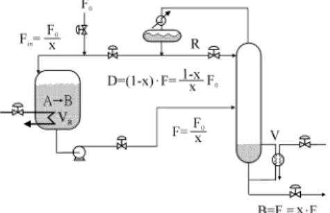
2.1. Process and Design Alternatives. A simple reactor/separator process is used to illustrate the effects of design and control structure selection.21,28,29 The process consists of a reactor and a distillation column in an interconnected structure as shown in Figure 1. The reaction is irreversible, A f B, with first-order kinetics.
Here R is the reaction rate (mol/h), k is the rate constant (h-1), VRis the reactor holdup (mol), and zAis the mole fraction of the reactant A. The effluent of the reactor (F in mol/h) is fed into a distillation column. The product B is removed from the bottom of the column. The purified reactant is recycled back to the reactor via the distillate flow. Note that, unless otherwise mentioned, all compositions and holdups are expressed in terms of mole fraction and moles. Figure 1 describes the flow rates in the recycle process under different reactor conversion (x).
Note that these flow rates are obtained from material balances with the assumptions of perfect separation and pure reactant (i.e., zA0 ) 1).
The conversion (x) is the dominant design variable for the simple recycle process. We can design the reactor with a small conversion (x) coupled with a distillation column large in diameter (for increased vapor/liquid flows), or one can make the reactor conversion large, connected to a moderately sized (in diameter) column. Note that the Fenske equation shows that the tray numbers are the same as long as the separation specifications remain the same. Steady-state economics of these alternatives are important in process design,15 but we are interested in recycle dynamics at the design stage.
Before we get into the model derivation, three plant-wide control principles are contrasted. In addition to necessary level and composition loops in plantwide control, one of the most important decisions to make is to set the throughput manipulator.4,17 Thus, we have to decide which variable should handle the production rate changes. As can be seen from eq 1, three likely candidates are reactor composition (changing zA via recycle flow4,14,15), reactor holdup (changing V
R28,29), and
reactor temperature (changing k via reactor tempera-ture). In a general way, these three control principles are termed as control structure 1 (CS1), control struc-ture 2 (CS2), and control strucstruc-ture 3 (CS3), respectively. The first case is studied here, and we will extend the other two cases in a later section.
2.2. Linear Model. CS1 is often referred to as the conventional structure, where the recycle flow is changed to accommodate production rate variation. This implies a constant reactor holdup.
2.2.1. Reactor. In a series of papers,6,16,18Luyben and co-workers investigated tradeoffs between design and control of chemical reactor systems. A similar approach is taken here with different definitions on state vari-ables. Consider the reactor in Figure 1 where Finis the reactor feed, F is the reactor effluent, and VR is the reactor holdup. The component material balance for A is
Generally, reactant concentrations, zAand zB, are state variables. However, in the analysis of the recycle process, it is more convenient to use the total outflow of components A and B, FAand FB, as state variables.
Assuming perfect level control (VR ) constant and Fin) F) and a pure reactant (zA0) 1) and substituting eq 4 into the balance equation (eq 3), we have
Linearizing eq 5 and taking Laplace transformation, one obtains
where the overbar stands for a nominal steady-state value. Note that, to obtain a correct linearization result, the time derivative of F in the left-hand side of eq 5 is treated as an independent variable. Because we would like to characterize the reactor size using the conversion, assuming pure reactant A and from steady-state mate-rial balances, we have
where τRis the reactor residence time. When eqs 4 and 7 are substituted into eq 6, the relationship between the total outflow of A and the total reactor feed becomes Figure 1. Reactor/separator recycle process.
dVRzA dt ) FinzA0- FzA- kVRzA (3) FA) FzA and FB) FzB (4) dFA dt -FA F dF dt ) F 2 VR -FFA VR - kFA (5) FA(s) F(s) ) FA F s +
(
2F VR -FA VR)
s +(
F VR + k)
(6) τR) VR F ) x k(1 - x) (7) FA(s) Fin(s)) x(1 - x) k s + (1 - x 2 ) x ks + 1 (8) R ) VRkzA (1) x )zA0- zA zA0 (2)A similar result can be obtained for component B.
Note that the steady-state gains in eqs 8 and 9 are different from those of the composition-based expres-sion. Equations 8 and 9 clearly indicate that an in-creased conversion, indeed, slows down the reactor dynamics as seen in the movement of the pole location (p ) -k/x where p denotes pole). It reveals that, at low conversion, the pole is located at the far left of the s plane and, as the conversion increases, the pole ap-proaches -k. Moreover, the low limit of the reactor dynamics is characterized by the fundamental chemis-try, the reaction rate constant (p ) -k).
2.2.2. Recycle Plant. With appropriate parametriza-tion, we can incorporate the reactor models into the recycle process. The recycle process consists of a reactor and a separator (Figure 1). Assuming perfect separation
with no separator dynamics, all of the unreacted
reac-tant A (FA) is recycled back to the reactor and the product B (FB) is taken out from the separator instan-taneously. Therefore, a block diagram can be con-structed to describe the recycle process. Note that this work differs from the previous modeling in that the outflows of different components (FAand FB) are used as state variables and the interaction between flow (F) and composition (zAand zB) can be avoided.
Figure 2A describes the basic idea where the reaction/ separation dynamics is lumped together for the recycle part (GR for reactant A) and for the product part (GP for product B) and the reactor flow dynamics (GL) is placed between the reactor influent and effluent. Be-cause perfect level control is assumed, we have
With the perfect separation assumption, the recycle flow and product flow dynamics are
Notice that if separator dynamics is not negligible and separation is far from perfect, additional lags and
separation gains (fractional recovery) can be included in GR and GP. Substituting the analytical expressions (eqs 8 and 9) into the positive feedback structure (Figure 2B), we are able to analyze the dynamics for the recycle process with alternative process designs.
where F0 denotes the fresh feed, P stands for the production rate, and D is the recycle flow. Several observations can be made from these immediately.
1. Regardless of the design alternatives (different conversions), perfect production changes can always be achieved as shown in Figure 3. Equation 13 defines the
input/output dynamics.
2. For different conversions (x) in design, the poles of
internal flow dynamics [D(s)/F0(s) and F(s)/F0(s)] are invariant and they are located at p ) -k as shown in parts B and C of Figure 3.
3. The zeros of internal flow dynamics [D(s)/F0(s) and F(s)/F0(s)] start from far left at low conversion (x f 0) and converge to -2k and -k at high conversion (x f 1) for recycle and reactor feed flow dynamics, respectively (parts B and C of Figure 3).
4. The steady-state sensitivity of the recycle flow (D) to the fresh feed flow (F0) varies from infinity to 0 as the conversion (x) changes from 0 to 1 as indicated by Figure 2. Conceptual description (A) and block diagram (B) for
the reactor/separator process.
FB(s) Fin(s) ) x2 ks + x 2 x ks + 1 (9) GL(s) ) 1 (10) GR) FA(s)/F(s) (11) GP) FB(s)/F(s) (12)
Figure 3. Root locus with varying conversion for the reactor/
separator process with CS1 for (A) product flow dynamics (× indicating a fixed pole), (B) recycle flow dynamics (× indicating a fixed pole and O denoting converging zero location), and (C) reactor flow dynamics (× indicating a fixed pole and O denoting converging zero location).
P(s) F0(s)) GLGP 1 - GLGR) 1 (13) D(s) F0(s)) GLGR 1 - GLGR) 1 - x kx s + 1 - x2 x2 1 ks + 1 (14) F(s) F0(s)) GL 1 - GLGR) 1 kxs + 1 x2 1 ks + 1 (15)
the steady-state gain, eq 14. In terms of absolute flow rates, the ratio is D/F0) (1 - x2)/x2and, expressed in percent deviation, the ratio becomes (D/D)/(F0/F0) ) (1 + x)/x.
It should be emphasized here that these observations are obtained under the assumptions of perfect level control and perfect separation. Observation 1 confirms
the remarks made by Luyben:15All of these competing effects result in a process in which the dynamics of various alternative designs are quite similar. However,
it is derived analytically here, and it is the most important result of this work because it points out that all different designs result in exactly the same input/ output dynamics as long as they are assembled into the recycle structure and, subsequently, perfect production control can be achieved. The reason is that the fast reactor dynamics (with small conversion) compensates the slow dynamics that comes from large recycle (large recycle gain, e.g., eq 14). However, the internal dynam-ics is different; the zero dynamdynam-ics varies with conversion (x) with a fixed pole location (p ) -k), as can be seen from eqs 14 and 15. Observation 4 confirms the sensi-tivity problem of recycle plants at low conversion, termed by Luyben17 as the “snowball effect”. For ex-ample, for a recycle process with a conversion of 0.1 (x ) 0.1), the recycle flow will increase 110% [(1 + 0.1)/ 0.1 ) 11] in order to accommodate a 10% step increase in the fresh feed flow.
2.3. Dynamic Responses. To illustrate recycle dy-namics, three design alternatives for the simple recycle process (Table 1) are studied. Because of the perfect separation assumption, parameter values are modified slightly. They belong to low conversion (x ) 0.2), moderate conversion (x ) 0.5), and high conversion (x ) 0.9). The dashed lines in Figure 4 show the responses of the linear model. As expected, perfect production rate tracking can be obtained for all three designs, while the internal dynamics (recycle flow D and reactor feed Fin ) F) follows similar dynamics with a time constant of
Table 1. Parameter Values and Steady-State Conditions for Reactor/Separator Systems
x ) 0.2 x ) 0.5 x ) 0.9
CSTR
fresh feed flow rate (F0) (lb‚mol/h) 460 460 460
fresh feed composition (z0) 0.9 0.9 0.9
fresh feed temperature (T0) (°R) 530 530 530
recycle flow rate (D) (lb‚mol/h) 2421 500.4 48.44 recycle stream composition (xD) 0.95 0.95 0.95
recycle stream temperature (TD) (°R) 587.2 587.2 587.2
reactor temperature (T) (°R) 616.4 616.4 616.4 reactor holdup (VR) (lb mol) 1501 2401 12005
activation energy (E) (Btu/lb‚mol) 30842 30842 30842 Distillation
column feed flow rate (F) (lb‚mol/h) 2881 960.4 508.4 column feed composition (zA) 0.8 0.5 0.1
reflux flow rate (R) (lb‚mol/h) 1861 1100 599 vapor boilup (V) (lb‚mol/h) 4282 1600 648
no. of trays (NT) 20 20 20
feed tray (NF) 15 12 8
liquid hydraulic time constant (β) (s) 4 4 4 bottom holdup (MB) (lb‚mol) 275 275 275
reflux drum holdup (MD) (lb‚mol) 185 185 185
tray holdup (Mn) (lb‚mol/tray) 23.5 23.5 23.5
bottom composition (xB) 0.0105 0.0105 0.0105
bottom flow rate (B) (lb‚mol/h) 460 460 460
Figure 4. Reactor/separator dynamics for step change in feed flow with CS1 for different steady-state designs using a linear model
1/k (p ) -k). Because the zero is approaching the pole location at high conversion for the reactor feed flow dynamics, a near pole zero cancellation is observed for the case of x ) 0.9. As for the recycle flow sensitivity, for a 10% step increase in the production rate, the recycle flows increase 60%, 30%, and 21% (x ) 0.2, 0.5, and 0.9).
3. Validation and Dominant Variables on Recycle Dynamics
The simulation results presented in the previous section are obtained with the following assumptions: (1) linear reactor model, (2) perfect separation with no separator dynamics, (3) perfect reactor temperature control, and (4) perfect reactor level control (for the case with constant reactor holdup). These assumptions will be lifted gradually in the following sections.
3.1. Relaxation on Modeling Assumptions. 3.1.1. Nonlinear Reactor Model. A nonlinear isothermal continuous stirred tank reactor (CSTR) model (eq 3) is placed in the recycle structure (Figure 2), and the perfect reactor level control is still assumed for this case of fixed reactor holdup. Note that, using FAand FBas state variables and F as the disturbance variable, we have a bilinear type of equation for the reactor, as can be seen from eq 5. This facilitates the description for processes with recycle (the recycle branch is clearly defined), but the reactor model becomes nonlinear. This means that we model the recycle process as a nonlinear CSTR with a perfect separator with no recycle dynam-ics. Results indicate that, for a 1% step increase in the feed flow, we have responses very similar to those obtained from a linearized model (solid lines in Figure 4). The difference is more evident at low conversions, as can be seen in Figure 4. Nonetheless, a very good approximation can be achieved using the linearized model.
3.1.2. Rigorous Distillation. Instead of assuming perfect separation, a rigorous binary distillation column is employed at this stage. The model of the distillation is similar to that in the book of Luyben13where 2(N
T+ 2) ordinary differential equations were used to describe column dynamics and NTdenotes the total number of trays. A linear tray hydraulic of 4 s is assumed. The
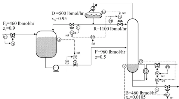
light reactant, A, is recycled back to the reactor, and the heavy product, B, is withdrawn from the bottom. The relative volatility is 2, and the product specification for the bottom is xB) 0.0105, mole fraction of the light component.28,29Parameter values for three alternative designs are given in Table 1. Perfect reactor level control is assumed for the time being. Figure 5 shows the process flowsheet for the recycle process with x ) 0.5. Because perfect level controls are assumed, we are left with one composition loop, controlling xBwith the boilup ratio. Relay feedback autotuning with a modified Zie-gler-Nichols tuning25is employed to find the controller gain (Kc) and reset time (τI) for the proportional-integral (PI) composition controller.
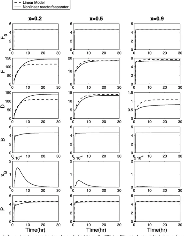
Simulation results, Figure 6, clearly show that an instantaneous production change (P) can be achieved for these nonlinear recycle processes, where P is the total production of the product B, i.e., P ) (1 - xB)B ) FB. Comparisons between a nonlinear column (solid lines) and perfect separation (dashed lines) are also made in Figure 6. Results reveal that the linear recycle models provide a very good description of the true process, especially for moderate to large conversions (e.g., x ) 0.5 and 0.9). Also notice that because perfect separation is assumed for the linear model, the recycle flow (D) and reactor effluent (F) are different in these two cases, but the dynamics is quite similar for both flows in these two cases.
3.2. Effect of Reactor Temperature Control. The interaction between the size and stability of the reactor is a practically important subject especially for reactor temperature control. Luyben and co-workers have stud-ied this subject with respect to scale-up,6 reactor con-figurations,16and autorefrigerated reactors.18The source of the problem is that, for a given aspect ratio, the reactor surface area (heat removal capacity) is related directly to the square of the reactor diameter while the reactor volume (heat generation) is related to the third power of the reactor diameter and, therefore, scaling up of the reactor size gives a relative reduction in the heat transfer capacity per unit volume. However, the reactor sizing problem for a recycle plant differs from the scale-up problem in that the conversion is varying. The appendix shows that, for a recycle plant, at low conver-Figure 5. Control structure for the reactor/separator process (PI level controller for CS1 and P-only level controller for CS2).
sion the reactor is less controllable and the controllabil-ity improved toward high conversion. The next question then becomes, how will this affect the control of a recycle plant?
Simulation results in Figure 7 show that, indeed, better reactor temperature control can be obtained at higher conversion (see the second row of Figure 7). However, again, almost perfect production rate changes (P) can be achieved for all three conversions. Figure 5 also compares perfect (dashed lines) reactor tempera-ture control to the nonperfect (solid lines) reactor temperature control case. Results reveal that, except for the temperature dynamics, the rest of the dynamic responses are almost identical. At least for these open-loop stable reactors, reactor temperature dynamics has little impact on the overall process dynamics. As a result, the reactor temperature control will not be
addressed further in this work. Nonetheless, it is interesting to notice the controllability trend for the reactor in a recycle plant because it is just the opposite to that of reactor scaling up. In other words, in a recycle plant, a larger reactor is easier to control.
3.3. Effect of Reactor Level Control. Finally, the assumption of perfect reactor level control is relaxed. Consider the reactor level control in Figure 5 with a PI controller. The closed-loop transfer function between Fin and F is simply
This is a second-order system, and we would like to Figure 6. Reactor/separator dynamics for step change in feed flow with CS1 for different steady-state designs using a linear model
(dashed lines) and a rigorous reactor/separator model + perfect reactor level control (solid lines).
GL(s) ) F Fin ) τ1s + 1 τ1 KC s2+ τ1s + 1 (16)
place the poles such that the system has a closed-loop time constant as a fraction of the residence (i.e., τCL) γτR) with a damping coefficient of ζ ) 0.707. This can be written as
After eq 7 is substituted for τRin eq 26, the controller
parameters can be expressed as
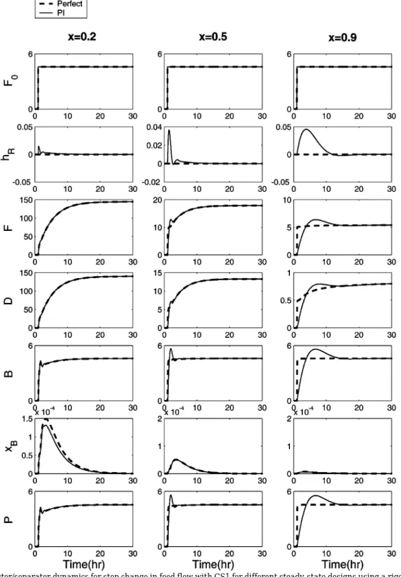
If we set γ ) 0.1 (i.e., τCL) 0.1τR) and ζ ) 0.707, Figure 8 shows that the dynamic responses slow as the conver-sion increases (e.g., dashed lines in Figure 8 with x ) 0.5 and 0.9). Figure 8 also reveals that perfect produc-Figure 7. Reactor/separator dynamics for step change in feed flow with CS1 for different steady-state designs using a rigorous reactor/
separator model assuming perfect reactor temperature control (dashed lines) and nonperfect reactor temperature control (solid lines).
GL(s) ) 2τCLσs + 1 τCL 2 s2+ 2τCLσs + 1 ) 2× 0.707(γτR)s + 1 (γτR) 2 s2+ 2 × 0.707(γτR)s + 1 (17) KC)x 2 γ k(1 - x) x (18) τI) x2xγ k(1 - x) (19)
tion rate changes can no longer be achieved, especially at high conversion.
With a PI reactor level control, the production rate dynamics in the recycle structure become
This is a third-order system with the net order of 1. With the typical tuning constants, the root locus plot of the conversion (x varying from 0 to 1) is shown in Figure 9. It shows that, initially, the first pole (p1) starts from the far left of the real axis and the other two poles are located at finite positions (p2, p3 ) k(-1 (
x
1-4γ2)/2γ2). The first two poles (p1and p2) converge to the origin as the conversion increases, and the third pole (p3) does not move much and was eventually canceled out by the zero (z ) -k in eq 20) as the conversion approaches 1 (i.e., x f 1). The analysis
P(s) F0(s) )
[
2xγ x2k(1 - x)s + 1]
(
1 ks + 1)
γ2x k3(1 - x)2s 3+[
γ2 k2(1 - x)2+ 2xγ x2k2 (1 - x)]
s 2+[
2xγ x2k(1 - x)+ 1k]
s + 1 (20)Figure 8. Reactor/separator dynamics for step change in feed flow with CS1 for different steady-state designs using a rigorous nonlinear
clearly indicates that, with a specification of γ ) 0.1 and
ζ ) 0.707 for the reactor level, the production dynamics
becomes slower as the conversion increases and will eventually reach the origin as shown in Figure 9, and this explains the discrepancy between the perfect level control and PI level control. The difference becomes more evident at high conversion (e.g., x ) 0.9 in Figure 8).
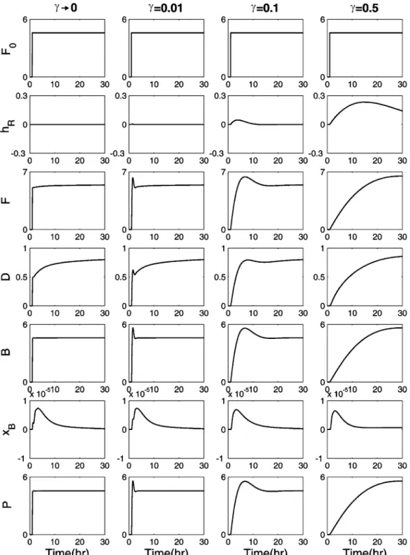
Equation 20 indicates that the closed-loop time con-stant (τCL) γτR) is effective in adjusting the production dynamics. If γ is set to zero, we have a perfect reactor level control as well as perfect production control, i.e., (P/F0)(s) ) 1, and if we increase γ, the poles move toward the origin as shown in Figure 10. This was confirmed by nonlinear simulation of the recycle process, where Figure 11 clearly indicates that the production dynamics becomes slower when we slowly increase γ. For x ) 0.9, the time constant of the total production (P) changes from 0 to 10 h as γ varies from 0 to 0.5 (Figure 11). Therefore, the reactor level control is crucial for the input/output dynamics of recycle processes and, for the case of high conversion, we can tighten the level loop tunings by specifying the dominant pole placement location for overall production dynamics (eq 20). To maintain a faster dynamic response, the closed-loop time constant to the residence time ratio (γ) has to be changed for different conversions. Here, we set the real part of the dominant pole at a specific location, as indicated by the vertical dashed line in Figure 10A, and this is equivalent to γ ) 0.01 for the case of x ) 0.9. Figure 12 compares the dynamics of perfect level control, using original tuning (i.e., typical tuning for the reactor level), and tightens the reactor level tuning. The results show that almost perfect production dynamics can be obtained by tightening the reactor level loop. 4. Extension to the Balanced Control Structure (CS2)
4.1. Linear Analysis. This class of control structures uses the reactor holdup to handle production rate variation,17,28,29and it is termed the balanced control structure. As shown by Wu et al.,29a simple
implemen-tation of the balanced control structure is to use a P-only controller for the reactor level, with the reactor effluent as the manipulated variable while the controller gain is set to KC ) 1/τR. In doing this, the reactor holdup change is proportional to the flow variation. In other words, we are keeping a constant residence time (τR) VR/F). After substituting the overall material balance into eq 7 for the residence time, we have
4.1.1. Reactor. The basic difference between these two structures lies in the reactor level control strategy. In the conventional structure, reactor holdup is fixed and, in the present case, the residence time (τR) VR/F) is kept constant. Following a similar approach, the component material balance equation (eq 2) can be linearized first, followed by taking Laplace transforma-tion. Thus, one obtains
The results indicate that the systems have two poles. The first one, the same as the previous case, is located at p1 ) -k/x, and the second one is p2 ) -k(1 - x)/x. Both poles start at the far left at low conversion and, at high conversion, the first pole (p1) converges to -k while the second pole (p2) moves toward the imaginary axis. This implies that the reactor dynamics can be extremely slow at high conversion. The reason for this slowdown comes from the large reactor residence for high conversion.
4.1.2. Recycle Plant. If we separate the reactor level dynamics from the level dynamics, the transfer func-Figure 9. Root locus plot with varying reactor conversion (x changing from 0 to 1) for the reactor/separator process with CS1 and a
typical reactor level control setting (γ ) 0.1).
F(s) Fin(s)) 1 τRs + 1 ) 1 x k(1 - x)s + 1 (21) FA(s) Fin(s)) 1 - x x ks + 1 (22) FB(s) Fin(s) ) x
(
x ks + 1)
[
x k(1 - x)s + 1]
(23)tions in the recycle block diagram (Figure 2) are
Substituting these transfer functions into the positive feedback structure, we have the following recycle dy-namics. Note that this is obtained by assuming perfect
separation with no recycle dynamics.
Some observations can be made immediately. 1. As the conversion increases, one of the poles (p2in Figure 5A) of the product flow dynamics moves from the far left toward the origin. Equation 27 clearly shows that the input/output dynamics become slower as the conversion increases.
2. For different conversions (x) in design, the pole of
recycle flow dynamics [D(s)/F0(s)] is invariant and it is located at p ) -k as shown in Figure 5B.
3. As the conversion (x) increases, one of the poles (p2) of reactor effluent dynamics [F(s)/F0(s)] moves toward the origin while the zero converges to z ) -k (Figure 5C).
4. The steady-state sensitivity of the recycle flow (D) to the fresh feed flow (F0) varies from infinity to 0 as the conversion (x) changes from 0 to 1, as indicated in eq 28. In terms of absolute flow rates, the ratio is D/F0 ) (1 - x)/x and, expressed in percent deviation, the ratio becomes (D/D)/(F0/F0) ) 1.
Obviously, for a recycle structure (Figure 2), the level control strategies lead to totally different recycle dy-namics. Perfect production control is no longer achiev-able under the case of variachiev-able reactor holdup. At small conversion, the recycle dynamics is comparable to that of the case of fixed reactor holdup. As the conversion increases (i.e., a larger reactor), the residence time increases and slower dynamics results (eq 16), as shown in Figure 13. However, the sensitivity of the recycle flow to the production rate variation, the snowball effect, is alleviated as indicated in observation 4. Actually, the percent change in the recycle flow is exactly the same as that of the feed flow, and this is exactly the objective of the balanced control structure, handling production rate changes using the reactor holdup.
4.1.3. Dynamic Responses. Again, three design alternatives for the simple recycle process are studied, and they belong to low conversion (x ) 0.2), moderate conversion (x ) 0.5), and high conversion (x ) 0.9). The dashed lines in Figure 14 indicate that slower produc-tion dynamics is observed at high conversion (e.g., x ) 0.9 in Figure 14). The recycle flow dynamics is about the same for all three conversions, while the reactor effluent dynamics follows a similar pattern as that of production dynamics. As for the recycle flow sensitivity, the recycle flows increase 10% (x ) 0.2, 0.5, and 0.9) for a 10% step increase in the production rate.
4.2. Validation. 4.2.1. Nonlinear Reactor. Because the production rate variation is handled by changing the reactor holdup, the reactor level dynamics has a time constant of τRwith a proportional gain of KC) 1/τR. Again, a nonlinear isothermal CSTR is assumed while using a perfect separator. For a 1% step increase in the Figure 10. Root locus plot with varying reactor level setting
(γ changing from 0 to 1) for different conversions (x ) 0.2, 0.5, and 0.9): (A) all three pole configurations (the dashed vertical line indicating γ ) 0.01, which is recommended for high conversion cases); (B) two zero configurations.
GL) 1 x k(1 - x)s + 1 (24) GR) (1 - x)
[
x k(1 - x)s + 1]
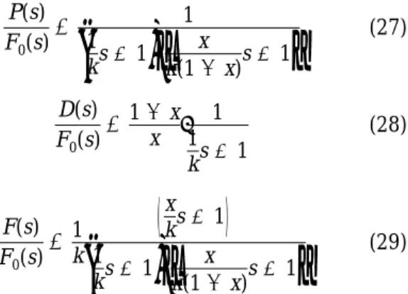
x ks + 1 (25) GP) x x ks + 1 (26) P(s) F0(s) ) 1(
1 ks + 1)
[
x k(1 - x)s + 1]
(27) D(s) F0(s)) 1 - x x ‚ 1 1 ks + 1 (28) F(s) F0(s) ) 1 k(
x ks + 1)
(
1 ks + 1)
[
x k(1 - x)s + 1]
(29)fresh feed flow, we have almost the same responses as those of a linearized model (solid lines in Figure 14). Again, a very good approximation can be obtained using the linearized model. Notice that as the step size increases (e.g., 5%), visible deviations in the recycle flows can be observed for the low conversion case (e.g.,
x ) 0.2) while the high conversion case still shows a
reasonably good behavior description.
4.2.2. Rigorous Distillation. Similar to the case of constant reactor holdup, a nonlinear distillation column is employed. This has exactly the balanced control structure of the recycle process studied in refs 4 and 29. Again, three alternative designs (low, moderate, and high conversions) are studied, and parameter values are
given in Table 1. The process flowsheet is exactly the same as Figure 5, but a P-only reactor level control is employed with KC) 1/τR. The composition controller is also set with the modified Ziegler-Nichols tuning.25
Simulation results clearly show that the production dynamics, P in Figure 15, become slower as the conver-sion increases. Figure 15 also reveals that much better composition control, xB, can be achieved as compared to that of the constant reactor holdup (xBin Figure 6), especially at low conversion, but with this dynamics, the total production is much slower compared to the case of constant reactor holdup (P in Figure 6). Results also reveal that the linear recycle models provide a very good description of the true process.
Figure 11. Rigorous reactor/separator dynamics for step change in feed flow with CS1 and x ) 0.9 using different degrees of tightness
5. Implications for Control
5.1. Tradeoffs between Steady-State Sensitivity and Dynamic Responsiveness. Rigorous nonlinear simulations confirm that the linear analysis (Figure 2) provides good behavior description for the recycle process and the observations in section 2 are generally valid for the material recycle process. These two control structures, CS1 and CS2 in Figure 5, possess different characteristics. In terms of dynamic responsiveness, near-perfect production rate variations can be achieved over the entire range of conversion for CS1 (e.g., Figure 12) and, for CS2, variable reactor holdup, sluggish production dynamics is observed at high conversion
(e.g., Figure 15). As for steady-state sensitivity, a severe snowball effect is observed for the control structure with constant VRand the sensitivity reaches infinity when the conversion approaches zero (e.g., observation 4 in section 2.1.2). This imposes an inherent limitation on the operability for CS1. For example, if the maximum flow rate of each stream is twice its nominal value (e.g.,
Fmax) 2Fh), it can be shown that the maximum percent-age of the production rate increase can be simply given by
Figure 12. Rigorous reactor/separator dynamics for step change in feed flow with CS1 and x ) 0.9 using perfect level control, conventional
reactor level tuning (keeping a fixed open-loop/closed-loop time constant ratio), and tightened reactor level tuning.
∆(P/P)max) 100
x
where x is the conversion. On the other hand, the operability for the CS2 control structure is much better
conversion. The variable reactor holdup (CS2) is pre-ferred at low conversion for its steady-state operability and not too slow dynamic responsiveness, and at moderate to high conversion, the constant VR(CS1) is a better choice for its dynamic responsiveness and acceptable steady-state operability. The boundary is determined by the turndown ratio of design. For ex-ample, if the maximum production rate is set to at least 125% of its nominal value (i.e., Pmax) 1.25Ph), from eq 30, we have x ) 0.25/(1 - 0.25) )1/
3. This implies that, if x <1/
3, the variable reactor holdup structure (CS2) is preferred and the constant VR(CS1) should be used for x g 1/
3. The thick solid lines in Figure 16 show the corresponding control structure at different conversions. 5.3. Ideal Control Structure. Can we devise a control structure such that the tradeoff between steady-state operability and dynamic responsiveness can be avoided? Before answering this question, it should be Figure 13. Root locus with varying conversion for the reactor/
separator process with CS2 for (A) product flow dynamics (× indicating converging pole and fixed pole locations), (B) recycle flow dynamics (× indicating a fixed pole), and (C) reactor flow dynamics (× indicating converging pole and fixed pole locations and O denoting converging zero location).
Figure 14. Reactor/separator dynamics for step change in feed flow with CS2 for different steady-state designs using a linear model
understood that the sluggishness in the production rate change originated from the reactor level dynamics and, for CS2, such a sluggish tuning comes from a change in the reactor holdup in proportion to the flow rate. Therefore, if we can handle the production rate variation using some variable without affecting flow dynamics, the tradeoffs can be eliminated. The reactor tempera-ture is one obvious choice, as shown in eq 1. This is exactly the third control structure (CS3) mentioned in section 2. Figure 17 shows that, in CS3, the production rate is set by the fresh feed flow and the reactor temperature is adjusted according to the fresh feed flow
via a feedforward controller. Similar to CS1, tight controller settings are required for the reactor level.
With the reactor temperature as the throughput manipulator (CS3), near-perfect production can be achieved while maintaining good steady-state oper-ability as shown in Figure 18, as compared to CS1. Certainly, CS3 is only applicable to the situation where a wide range of reactor temperature variation can be practiced.
Before leaving the section, one control strategy not addressed in the paper involves on-demand production rate. Here the base stream from the column is flow-Figure 15. Reactor/separator dynamics for step change in feed flow with CS2 for different steady-state designs using a linear model
controlled, with the setpoint coming from the down-stream unit that demands instantaneous rate changes. In this case what part of the analysis in this paper applies to this situation? The step input in the fresh feed results in a step output in the total production (considering CS1 with perfect reactor level control). This implies that, for the on-demand structure, perfect control can also be achieved if the fresh feed also shows a steplike input. This can be achieved by the proper design of the level controller (assuming using base level to control the column feed). That is the column base level controller should be able to give the following relationship:
If one chooses to use a ratio scheme [(D + F0)/P], the ratio controller should have the following dynamics:
analysis facilitates the evaluation of process dynamics at the design stage and, more importantly, input/output dynamics depends on the control structure. Therefore, a preliminary decision on the control structure, i.e., determining the throughput manipulator, has to be made to assess the dynamic performance at the design stage.
In this work a simple recycle process with a first-order irreversible reaction is studied. In the modeling phase, the total flows of different components (FAand FB) are parametrized as state variables, instead of using the typical composition (zAand zB). For the case of constant reactor holdup (CS1), as opposed to one’s intuition, linear analysis indicates that perfect production rate changes can always be achieved over the entire range
of conversion. The reason is that the effects of the
reactor dynamics and recycle gain compensate for each other, and perfect production is, thus, obtained for
input/output dynamics while the internal dynamics is
characterized as the rate constants (k). However, ex-treme steady-state sensitivity (also known as the snow-ball effect) is observed at low conversion. Linear analysis is validated using rigorous nonlinear simulations via a step-by-step relaxation on assumptions. The results also reveal the important role the reactor level dynamics play in dynamic responsiveness. and near-perfect input/ output dynamics can be obtained by tightening the reactor level settings.
This approach is extended to the balanced control structure (CS2), and results show that input/output Figure 16. Recommended control structure using the maximum
achievable production rate (Pmax) 1.25Ph) as a criterion: CS1 and
CS2.
Figure 17. CS3 control structure for the reactor/separator process using the reactor temperature to accommodate production rate variation. F(s) P(s)) GL 1 - GLGR ) 1 kxs + 1 x2 1 ks + 1
dynamics varies with conversion. In particular, when the convergence approaches unity (i.e., x f 1), an almost integrator response is observed. However, the steady-state sensitivity is invariant [i.e., (D/Dh )/(F0/Fh0) ) 1] over the entire range of conversion.
The proposed linear analysis clearly reveals tradeoffs between steady-state sensitivity and dynamic respon-siveness. It is further extended to devise an ideal control structure (CS3) to achieve dynamic responsiveness while maintaining steady-state operability.
Acknowledgment
Financial support of the National Science Council of Taiwan is gratefully acknowledged. FORTRAN code for the nonlinear recycle plant is available upon request. Appendix: Temperature Effect on
Controllability for a Reactor in a Recycle Plant Luyben15uses the temperature difference between the reactor (TR) and the jacket (TJ) as a measure of the robustness and flexibility of the reactor system (i.e., ∆T Figure 18. Reactor/separator dynamics for step change in feed flow for different steady-state designs using different control structures:
area, and only a small temperature difference is re-quired to remove the heat generated from the reaction. On the other hand, if A is too small, then a large ∆T will be needed to remove the heat. Also note that the heat-transfer area (A) is not an independent variable and it is a function of the reactor volume. Letting the aspect ratio of the reactor be n (i.e, n ) reactor height/ reactor diameter), the relationship between the jacket area (A) and reactor holdup VR(or volume) then becomes
where v is the molar volume (because the reactor holdup is in lb mol). Assuming a pure reactant and from eq A1, the controllability measure becomes
For a given fresh feed flow (F0), from eq 7 and the relationship between the conversion (x) and the reactor feed flow (F), VRcan be expressed as
Substituting eq B4 into eq B3, one obtains
Equation A5 is useful in evaluating reactor controllabil-ity for many possible scenarios. For a given production rate and reaction kinetics, the only design variable is the conversion (x), and eq A5 clearly indicates that a larger conversion implies a smaller ∆T and, thus, better controllability. This gives exactly the opposite results compared to the case of scaling up of a reactor.6
Nomenclature
A ) reactor jacket area
A ) reactant B ) product
B ) product flow rate (from the bottom of the distillation)
CS1 ) control structure with constant reactor holdup (using zAto handle the production rate variation) CS2 ) control structure with variable reactor holdup (using
VRto handle the production rate variation)
F0) nominal value of the fresh feed flow rate (mol/h)
GL(s) ) reactor level dynamics
GR(s) ) reaction and separation dynamics for reactant A
GP(s) ) reaction and separation dynamics for product B
k ) reaction rate constant
k0) preexponential factor for the rate constant
KC) controller gain
n ) aspect ratio of a reactor (height/diameter) pi) ith pole of a transfer function
P(s) ) total production rate [i.e., P ) (1 - xB)B ) FB] (mol/h)
P ) nominal value of the production rate (mol/h)
R(s) ) reflux flow rate in the distillation column (mol/h) R ) nominal value of the reflux flow rate in the
distilla-tion column (mol/h)
TJ) reactor jacket temperature
TR) reactor temperature
U ) overall heat-transfer coefficient v ) molar volume
VR) reactor holdup (mol)
x ) conversion in the reactor
xB) bottom product composition (mole fraction)
xD) distillate composition (mole fraction)
zA) reactor composition of A (mole fraction)
zB) reactor composition of B (mole fraction)
zi) ith zero of the transfer function
Greek Symbols
∆T ) difference between the reactor temperature and the jacket temperature (used as a controllability measure)
λ ) exothermic heat of reaction (a positive value) γ ) fraction of the residence time
τCL) closed-loop time constant (τCL) γτR)
τI) reset time
τR) residence time for the reactor
ζ ) damping coefficient
Literature Cited
(1) Bildea, C. S.; Dimian, A. C.; Iedema, P. D. Nonlinear Behavior of Reactor-Separator-Recycle Systems. Comput. Chem.
Eng. 2000, 23, 209.
(2) Chen, Y. H.; Yu, C. C. Interaction between Thermodynamic Efficiency and Dynamic Controllability: Heat-Integrated Reactor.
Comput. Chem. Eng. 2000, 23, 1077.
(3) Chen, Y. H.; Yu, C. C. Dynamical Properties of Product Life Cycle: Implications to the Design and Operation of Industrial Processes. Ind. Eng. Chem. Res. 2001, 40, 2452.
(4) Cheng, Y. C.; Wu, K. L.; Yu, C. C. Arrangement of Throughput/Inventory Control in Plantwide Control. J. Chin. Inst.
Chem. Eng. 2002, 33, 283.
(5) Denn, M. M.; Lavie, R. Dynamics of Plants with Recycle.
Chem. Eng. J. 1982, 24, 55.
(6) Devia, N.; Luyben, W. L. Reactors: Size versus Stability.
Hydrocarbon Process. 1978, 57 (6), 119. A ) (16nπ)1/3v2/3VR2/3 (A2) ∆T ) kVR(1 - x)λ U(16nπ)1/3v2/3VR2/3 ) kλ U(16nπ)1/3v2/3(1 - x)VR 1/3 (A3) VR) Fx k(1 - x)) F0 k(1 - x) (A4) ∆T ) kλ U(16nπ)1/3v2/3(1 - x)
[
F0 k(1 - x)]
1/3 ) λF0 1/3 k2/3 U(16nπ)1/3v2/3(1 - x) 2/3 (A5)(7) Gilliland, E. R.; Gould, L. A.; Boyle, T. J. Dynamic Effects of Material Recycle. Proceedings of the Joint Automatic Control Conference, Stanford University, 1964; p 140.
(8) Jacobsen, E. W. On the Dynamics of Integrated Plantss Non-Minimum Phase Behavior. J. Process Control 1999, 9, 439. (9) Kapoor, N.; McAvoy, T. J.; Marlin, T. E. Effect of Recycle Structure on Distillation Tower Time Constants. AIChE J. 1986,
32, 411.
(10) Kiss, A. A.; Bildea, C. S.; Dimian, A. C.; Iedema, P. D. State Multiplicity in CSTR-Separator-Recycle Polymerisation Systems.
Chem. Eng. Sci. 2002, 57, 535.
(11) Kwok, K. E.; Chong-Ping, M.; Dumont, G. A. Seasonal Model Based Control of Processes with Recycle Dynamics. Ind.
Eng. Chem. Res. 2001, 40, 1633.
(12) Lakshminarayanan, S.; Takada, H. Empirical Modelling of Processes with Recycle: Some Insights via Case Studies. Chem.
Eng. Sci. 2001, 56, 3327.
(13) Luyben, W. L. Process Modeling, Simulation, and Control
for Chemical Engineers, 2nd ed.; McGraw-Hill: New York 1989.
(14) Luyben, W. L. Dynamics and Control of Recycle Systems. 1. Simple Open-Loop and Closed-Loop Systems. Ind. Eng. Chem.
Res. 1993, 32, 466.
(15) Luyben, W. L. Dynamics and Control of Recycle Systems. 2. Comparison of Alternative Process Designs. Ind. Eng. Chem.
Res. 1993, 32, 476.
(16) Luyben, W. L. Trade-offs between Design and Control in Chemical Reactor Systems. J. Process Control 1993, 3, 17.
(17) Luyben, W. L. Snowball Effect in Reactor/Separator Pro-cess with Recycle. Ind. Eng. Chem. Res. 1994, 33, 299.
(18) Luyben, W. L. Temperature Control of Autorefrigerated Reactors. J. Process Control 1999, 9, 301.
(19) Morud, J.; Skogestad, S. Dynamic Behavior of Integrated Plants. J. Process Control 1996, 6, 145.
(20) Ogunnaike, B. A.; Ray, W. H. Process Dynamics, Modeling
and Control; Oxford University Press: Oxford, U.K., 1994.
(21) Papadourakis, A.; Doherty, M. F.; Douglas, J. M. Relative Gain Array for Units in Plants with Recycle. Ind. Eng. Chem. Res. 1987, 26, 1259.
(22) Pushpavanam, S.; Kienle, A. Nonlinear Behavior of an Ideal Reactor Separator Network with Mass Recycle. Chem. Eng.
Sci. 2001, 56, 2873.
(23) Scali, C.; Ferrari, F. Performance of Control Systems Based on Recycle Compensators in Integrated Plants. J. Process Control 1999, 9, 425.
(24) Seborg, D. E.; Edgar, T. F.; Mellichamp, D. A. Process
Dynamics and Control; Wiley: New York, 1989.
(25) Shen, S. H.; Yu, C. C. Use of Relay-Feedback Test for Automatic Tuning of Multivariable Systems. AIChE J. 1994, 40, 627.
(26) Taiwo, O. The Design of Robust Control Systems for Plants with Recycle. Int. J. Control 1993, 43, 671.
(27) Verykios, X. E.; Luyben, W. L. Steady-State Sensitivity and Dynamics of a Reactor/Distillation Column Systems with Recycle.
ISA Trans. 1978, 17 (2), 31.
(28) Wu, K. L.; Yu, C. C. Reactor/Separator Processes with Recycles1. Candidate Control Structure for Operability. Comput.
Chem. Eng. 1996, 20, 1291.
(29) Wu, K. L.; Yu, C. C.; Luyben, W. L.; Skogestad, S. Reactor/ Separator Processes with Recycles2. Design for Composition Control. Comput. Chem. Eng. 2003, 27, 421.
Received for review October 10, 2002 Revised manuscript received June 9, 2003 Accepted July 11, 2003