Motion of a Colloidal Particle Coated with a Layer of Adsorbed Polymers in a Spherical Cavity

(1)

ARTICLE NO.CS964594

Motion of a Colloidal Particle Coated with a Layer of Adsorbed

Polymers in a Spherical Cavity

HUANJ. KEH1ANDJIMMYKUO

Department of Chemical Engineering, National Taiwan University, Taipei 106-17 Taiwan, Republic of China

Received April 15, 1996; accepted September 9, 1996

to the effective decrease in size (15). The attachment of

An analytical study is presented for the quasisteady translation _{polymers to microporous membranes offers the possibility} and steady rotation of a spherical particle covered by a layer of

of manipulating the transport rate of solvent and solutes

adsorbed polymers located at the center of a spherical cavity that

and negating the adverse effects of pore-size distribution on

may also have an adsorbed polymer layer on its inside wall. The

membrane separations (16).

Reynolds number is assumed to be small, and the surface polymer

The structure of an adsorbed polymer layer depends on

layers are assumed to be thin with respect to the particle radius

the nature of the polymer, the solvent, and the interface. In

and the spacing between solid surfaces. To solve the Stokes flow

general, the adsorbed polymer chains consist of a collection

equations within and outside the polymer layers a method of

of ‘‘trains,’’ in which each polymer segment contacts the

matched asymptotic expansions in small parameters l1and l2is

used, where l1and l2are the ratios of the polymer-layer length interface, ‘‘loops,’’ in which only the initial and final

seg-scale to the radius of curvature at the particle surface and at the _{ments attach to the interface, and ‘‘tails,’’ which begin at} cavity wall, respectively. The results for the hydrodynamic force _{the interface but terminate in the solution (17, 18). Since} and torque exerted on the particle are expressed as an effective _{the adsorbed polymer layer is diffuse, there is no unique} hydrodynamic thickness (L) of the adsorbed polymer layer

sur-measure of its thickness. One convenient definition,

applica-rounding the particle, which are accurate to O(l2

1). The O(l1) term

ble to both colloidal particles and micropores, is the

hydro-for L normalized by its value in the absence of the cavity is found

dynamic thickness which is the distance the ‘‘no-slip’’

to be independent of the polymer segment distribution, the

hydro-boundary condition on the fluid velocity must be moved into

dynamic interactions among the segments, and the volume

frac-the fluid phase to produce frac-the same hydrodynamic effect as

tion of the segments. The O(l2

1) term for L, however, is a sensitive

the polymer layer. For the case of a polymer layer that is

function of the polymer segment distribution and the volume

frac-thin relative to the radii of curvature of the solid surface,

tion of the segments. In general, the boundary effects on the motion

of a polymer-coated particle can be quite significant in appropriate previous theoretical analyses (19 – 21) predict the same value

situations. q 1997 Academic Press of the hydrodynamic thickness for different external flows

Key Words: particle translation; particle rotation; adsorbed poly- _{and geometries, given the same local rheological model for}

mers; hydrodynamic thickness; boundary effects. _{flow within the surface layer. It has been found both}

theoreti-cally (19) and experimentally (22) that the hydrodynamic thickness is often much larger than the layer thickness

deter-1. INTRODUCTION _{mined optically by ellipsometry or by neutron scattering.}

The effects of adsorbed polymers on the steady translation The adsorption of polymers at solid – liquid interfaces is

and steady rotation of a single spherical particle were deter-of practical interest in various fields and has been a subject

mined by Anderson and Kim (21) using a method of matched of many theoretical (1 – 6) and experimental (7 – 12)

investi-asymptotic expansions to solve the Stokes flow equations gations. Coating of colloidal particles with polymers plays

within and outside the polymer layer. The results for the an important role in the control of the stability/flocculation

drag force and torque produced by the fluid on the particle, behavior of colloidal suspensions (13). The interactions

be-expressed as the hydrodynamic thickness of the adsorbed tween polymer and particle generate nonuniform

distribu-polymer layer, are accurate to O(l2

1) where l1is the ratio of

tions of polymer throughout the solution and influence the

the polymer-layer length scale to the particle radius. Their energy between particles (14). Another spectacular effect of

calculations indicated that (i) the O(l2

1) term is negative,

such adsorption is the restriction of flow in capillaries due

meaning the hydrodynamic thickness decreases as the parti-cle radius decreases assuming all other conditions are con-1

(2)

polymer chains applies accurately for calculating the hydro- vector in the positive z (axial) direction. The Reynolds num-ber is assumed to be small.

dynamic thickness if the Stokes radius of the polymer

seg-ments is much smaller than the length scale of the polymer The fluid flow between the particle and the cavity is gov-erned by the modified Stokes equations (21):

layer, and (iii) the presence of only a small amount of ad-sorbed polymer tails can make a significant contribution to the hydrodynamic thickness if the length scale of the tails _Çr

{m[Ç_v_{J /}₍Ç_v_J₎T

]}0 Çp0zrf [v_{J 0}v_J(p)

] Å0_J, [2.1a] exceeds the length scale of the loops by a factor of 2 or

more. Çrv_{J Å}0. [2.1b]

In many practical situations, colloidal particles are not isolated and will move in the presence of neighboring

parti-Here, v_J is the fluid velocity, p is the hydrodynamic pressure, cles and/or boundaries. Although the translational and

rota-z is the friction coefficient of an isolated polymer segment,

tional motions of a colloidal sphere coated with a layer of

r is the density of polymer segments at the position in

ques-adsorbed polymers in an unbounded liquid were analyzed

tion, v_J(p)

is the velocity of the segments, f is a function of (21), the boundary effect on the movement of such particles

r accounting for the hydrodynamic interactions among the

has not yet been reported. The purpose of this work is to

segments, and m is the local fluid viscosity which also varies obtain insights into the boundary effects on the motion of a

with r. Previous studies (1, 2, 17) established that the density polymer-coated particle within a small pore. This type of

of polymer segments in the loops decays exponentially with problem is difficult to solve due to the structural difference

the distance from the solid surface and the segment density for hydrodynamics within and outside the polymer layer and

in the tails can exceed the value in the bulk solution much the complexity of the actual system geometry. In order to

farther from the surface. For a free-draining model for flow avoid the mathematical difficulties encountered in the sphere

through the segments fÅ1, while segment – segment interac-and cylindrical pore problem, we choose to study the

transla-tions cause f to increase with r. It is understood that vJ(p) _Å

tional and rotational motions of a spherical particle

sur-0J in the polymer layer adjacent to the stationary cavity wall rounded by an adsorbed polymer layer located at the center

and v_J(p)

ÅUe_Jzin the surface layer surrounding the translating

of a spherical cavity that may also bear a layer of adsorbed

particle. polymers on its inside wall. Although the geometry of

spher-Since the flow field is axially symmetric, it is convenient ical cavity is an idealized abstraction of any real system, the

to introduce the Stokes stream function C which satisfies results obtained in this geometry have been shown to be in

Eq. [2.1b] and is related to the velocity components in the good agreement with available expressions for the boundary

spherical coordinate system (r, u, f), with its origin at the effects on the partition coefficient (23, 24), settling velocity

particle center, by (25, 26), and electrophoretic mobility (27, 28) of a ‘‘bare’’

particle in a cylindrical pore. Our analysis indicates that the boundary effects on the motion of a polymer-coated particle

vrÅ 0 1 r2 sin u ÌC Ìu , vuÅ 1 rsin u ÌC Ìr . [2.2a,b] can be significant in general situations.

2. TRANSLATION OF A PARTICLE

Taking the curl of Eq. [2.1a] and applying Eqs. [2.1b] and

IN A SPHERICAL CAVITY

[2.2] gives a fourth-order linear partial differential equation for C:

In this section we consider the quasisteady translational motion of a spherical particle of radius R1 in a concentric

spherical cavity (or pore) of radius R2filled with an

incom-mE4 C/ 2dm dr Ì Ìr(E 2 C)/2

S

rd 2 m dr2 0 dm dr

D

Ì Ìr

S

1 r ÌC Ìr

D

pressible Newtonian fluid. Both the surfaces of the particle

and of the inside wall of the cavity are covered by a layer of adsorbed polymers. The thicknesses of the two surface

polymer layers are characterized by length scales d1and d2 ₀d 2_m dr2 E 2 C0l02i

S

biE2C/ dbi dr ÌC Ìr

D

Å0, [2.3] (based on loops if both loops and tails are present), which

are assumed to be small in comparison with R1 and R2,

respectively, and with R2 0 R1. So, these two thin layers _{where i can be either 1 or 2, the dimensionless parameters}

will not overlap with each other. In general, the length scale _b

iand liare defined as

of a surface polymer layer depends on the molecular weight of the polymer, the amount of the polymer adsorbed, and

the relative interactions among the polymer, interface, and _b

iÅ d2 izrf ms , liÅ di Ri , [2.4a,b]

(3)

and the axisymmetric Stokesian operator E2

is given by The constants C0, D0, E0, and F0can be obtained by solving

for the corresponding motion of a ‘‘bare’’ spherical particle in a ‘‘bare’’ spherical cavity, with the result

E2 Å Ì 2 Ìr2/ sin u r2 Ì Ìu

S

1 sin u Ì Ìu

D

. [2.5] C0Å 1 4R 3 1(10l 3 )Ã, [2.12a]

In Eq. [2.3], dimensionless variables are used, with r normal-ized by the radius Ri, m by the solvent viscosity ms, and C

D0Å 0 3 4R1(10l 5 )Ã, [2.12b] by UR2

i. The parameter bidenotes the ratio of the frictional

force exerted by the polymer segments on the fluid to the viscous force of the bulk fluid, and is O(1) with respect to

E0Å 1 8(9l05l 3 04l6 )Ã, [2.12c]

liwhich has been assumed to be small. Equation [2.3] must

be solved subject to the following boundary conditions:

F0Å 0 3 8R 02 1 (l30l5)Ã, [2.12d] rÅR1: vJ ÅUeJz, [2.6a] where rÅR2: vJ Å0J. [2.6b] lÅR1 R2 ,Ã Å

S

109 4l / 5 2l 3 09 4l 5 /l6

D

01 . [2.13a,b] The drag force (in the z direction) exerted by the fluid on

the particle surface rÅR1is (26)

The unknown constants Cn, Dn, En, and Fnfor n§1 are to

be determined by matching C(O)

with the solution to Eq.

FdÅpms

*

p 0 r3 sin3 u Ì Ìr

S

E2 C r2 sin2

u

D

r du. [2.7] _{[2.3] in the ‘‘inner regions.’’ Combination of Eqs. [2.7] –}

[2.11] results in In terms of the equivalent hydrodynamic thickness L of the

adsorbed polymer layer surrounding the particle, the drag

A ÅD1

D0

, B ÅD2

D1

. [2.14a,b]

force is given by the Stokes law with a wall correction,

Within the ‘‘inner region’’ adjacent to the particle, where

FdÅ 06pms(R1/L)UK. [2.8]

r0R1ÉO(R1l1), a solution to Eq. [2.3] with the reference

frame moving with the particle is sought in the form For the system specified by Eq. [2.6], the wall correction

factor KÅ 04D0/3R1, where D0is defined by Eq. [2.12b].

C(I ) i Å[l 2 iFi2( yi) /l 3 iFi3( yi)/ rrr]U sin 2 u, [2.15] The hydrodynamic thickness of the polymer layer can be

expressed as

where iÅ1 and the variable y1Ål

01

1 (r0 R1). Within the

‘‘inner region’’ near the inside wall of the cavity, in which LÅAR1l1(1/Bl1)/O(l31). [2.9]

R2 0 r É O(R2l2), the solution to Eq. [2.3] can also be

written in the form of Eq. [2.15] with iÅ2 and the variable By combining Eqs. [2.7] – [2.9] after solving Eqs. [2.3] and

y2Ål

01

2 (R20r). Substituting Eq. [2.15] into Eqs. [2.3] and

[2.6] for C, one can obtain dimensionless parameters A and

[2.6] and collecting terms of equal orders in ligenerates the

B. Note that K § 1, A is positive, and B represents the

following equations for Fin(yi) up to nÅ 3:

correction for the particle curvature.

Equation [2.3] poses a singular perturbation problem when

l1!1 and l2! 1. In the ‘‘outer region,’’ where r0R1@ Ri

ms d dyi

S

md 2 Fi2 dy2 i

D

0bi Ri dFi2 dyi Å0, [2.16a]

R1l1and R20r@ R2l2, one has mÅmsand biÅ0 and the

solution can be written as

yiÅ0: Fi2Å dFi2 dyi Å0; [2.16b] C(O) Å(Cr01 /Dr/Er2 /Fr4 )U sin2 u, [2.10] CÅC0/l1C1/l 2 1C2 / rrr, [2.11a] Ri ms d dyi

S

md 2 Fi3 dy2 i

D

0bi Ri dFi3 dyi DÅD0/ l1D1/l 2 1D2/ rrr, [2.11b] E ÅE0/l1E1/l21E2/ rrr, [2.11c] Å(3 02i) 2 ms dm dyi dFi2 dyi 0ci, [2.17a] F ÅF0/l1F1/l21F2/ rrr. [2.11d]

(4)

Equation [2.19a] and the derivative of Eq. [2.19b] with yiÅ0: Fi3Å

dFi3

dyi

Å0, [2.17b]

respect to yiare immediately satisfied with the solution of

C0, D0, E0, and F0 given by Eq. [2.12]. The constants C1,

D1, E1, and F1can be determined by solving Eq. [2.19b] and

where i Å 1 or 2 and ci are integration constants to be

the derivative of Eq. [2.19c] with the knowledge of C0, D0,

determined by matching the inner and outer solutions.

E0, and F0, and then the constants C2, D2, E2, and F2are to

The unknown boundary conditions on Finat yir ` and

be determined by solving Eq. [2.19c] and the derivative of the unknown constants Cn, Dn, En, and Fncan be obtained

Eq. [2.19d]. The useful results are obtained in the following by matching Eqs. [2.10] and [2.15] at equivalent orders in

form: li: D1Å 0 1 3

∑

should be replaced by setting iÅ1. lim yir` d2 Fi3 dy2 i Å 0ci yi Ri /di. [2.24b]

In the limit of R2/R1r `, the boundary effect of the cavity

on the motion of the particle disappears and all the variables Knowing that m Å ms and bi Å 0 as yir `, one can find with subscript i Å 2 are irrelevant to the hydrodynamic

that Eqs. [2.16a] and [2.17a] are consistent with Eq. [2.24]. _{thickness of the polymer layer surrounding the particle. For}

If we define new variables _{this case, Eq. [2.23] gives b}₁Åc1Å3/2 and d1Å(3/2)g1,

and Eq. [2.28] reduces to

GiÅ 0 1 bi dFi2 dyi , HiÅ 0 1 ci dFi3 dyi , [2.25a,b] A` Åg1Å 1 R1 lim y1r` (G1/y1), [2.29a]

then Eqs. [2.16], [2.17], and [2.24] give

B` Å 1 R1g1 lim y1r`

S

H10 y2 1 2R1 /g1y1

D

Ri ms d dyi

S

m dGi dyi

D

0bi Ri GiÅ0, [2.26a] / 1 R2 1g1

*

` 0 (G1/y10R1g1)dy1. [2.29b] yiÅ0: GiÅ0, [2.26b]

Here, we use the subscript ‘‘`’’ to A and B to denote the yir `:

dGi

dyi

r 01; [2.26c]

limiting case of R2/R1r `. The numerical values of A`and

B` for various situations were given by Anderson and Kim

(21). In general, B` for translation of a particle would be

Ri ms d dyi

S

mdHi dyi

D

0bi mi Hi negative.

The drag force exerted on the particle written by Eq. [2.8] can also be expressed as

Å1/2(302i)bi ci Gi ms dm dyi , [2.27a] FdÅ 06pms(R1/L`)UK[1/gl1/hl21/O(l31)], [2.30] yiÅ0: HiÅ0, [2.27b] where yir `: dHi dyi r yi Ri 0di ci . [2.27c] L`ÅA`R1l1(1/B`l1)/O(l31). [2.31]

The two parameters of Eq. [2.9] are obtained from Eqs.

gÅ A0A_`, [2.32a] hÅ AB0A`B` 0A`(A0A`). [2.32b] / 1 Ri

*

` 0

(Gi/ yi0Rigi)dyi

G

. [2.28b] _{3. ROTATION OF A PARTICLE}

IN A SPHERICAL CAVITY

After the solutions of Eqs. [2.26] and [2.27] for given poly- We now consider the steady rotational motion of a spheri-mer segment density distributions r(yi) and the dependence cal particle covered by a layer of adsorbed polymers situated

of m and bion r are obtained, parameters A and B can be at the center of a spherical cavity which is also coated with

evaluated from Eq. [2.28]. a polymer layer on its inside wall. The angular velocity of

When there is no polymer adsorbed on the inside wall of the particle is VeJz. The fluid flow between the particle and

the cavity is still governed by Eq. [2.1], and it must be solved the cavity, one has d2Ål2ÅC(I)2 Å0. All of the variables

(6)

rÅR1: vJ ÅVr sin ueJf, [3.1a] p

(I )

i Åconstant, [3.7a]

r ÅR2: vJ Å 0J, [3.1b] vJ(I )_i Å[l_iF_i1*( y_i)/l2_iF_i2*( y_i)/ rrr]V sin ueJ_f, [3.7b]

where e_Jf is the unit vector along changes in the azimuthal _{where i}_Å_{1 and the variable y}

1Ål

01

1 (r0 R1). Within the

angle. _{inner region near the inside wall of the cavity, where R}

20

The effective hydrodynamic thickness L of the adsorbed _r_É_O(R

2l2), the solution to Eq. [2.1] can also be expressed

, [3.9a]

O(R2l2) respectively). In the outer region, we can write the

solution as

yiÅ0: F*i2Å0. [3.9b]

p(O) _Å

constant, [3.3a]

v_J(O) _Å

(Mr02/Nr)V sin ue_Jf, [3.3b] _{The unknown boundary conditions on F}_*

inat yir ` and

the unknown constants Mnand Nncan be obtained by

match-MÅM0/l1M1/l

2

1M2/ rrr, [3.4a]

ing Eqs. [3.3b] and [3.7b] at equivalent orders in li:

NÅN0/l1N1/l 2 1N2/ rrr. [3.4b] lim y1r` v_J(I )

1 Å[vJ(O) 0Vr sin ueJf]rrR1/l1y1, [3.10a] The constants M0and N0can be obtained easily by solving

for the corresponding motion of a spherical particle in a

lim

y2r` v_J(I )

2 Å[vJ(O)]rrR20l2y2. [3.10b] spherical cavity in the absence of adsorbed polymer layers,

with the result

The second term in brackets of Eq. [3.10a] accounts for the difference in the reference frames used for vJ(I )

1 and vJ(O). After

M0Å R3 1 10 l3, N0Å 0 l3 10l3, [3.5a,b]

performing this matching one obtains

where l was defined by Eq. [2.13a]. The unknown constants ₀_Å_W_*

i00(2 0i)R1, [3.11a]

Mnand Nnfor n§1 are to be determined by matching vJ

(O)

0R1ÉO(R1l1), a solution to Eq. [2.1] with the reference

(7)

where For given polymer segment density distributions r(yi) and

the dependence of m and bion r, the parameters A and B

of Eq. [2.9] can be obtained from Eqs. [3.6] and [3.13] after W*ik ÅR

02

i Mk/RiNk, [3.12a]

solving Eqs. [3.8], [3.9], and [3.16] for F*i1and F*i2.

When there is no polymer attached to the cavity wall, one X*ik Å 02R03i Mk /Nk, [3.12b]

has v_J(I)

2 Å0J. Then, all the variables with subscript iÅ2 are

Y*ik Å3R04i Mk, [3.12c] trivial except for R₂, and the summation symbol in Eq. [3.13]

should be replaced by setting iÅ1.

for iÅ1 or 2 and kÅ0, 1, or 2. _{In the limiting case of R}₂_/R₁ _{r `}_{, Eq. [3.15] gives b}_*₁ _Å

Solution of Eq. [3.11a] yields M0 and N0 given by Eq. _{3, c}*

1Å6, and d*1 Å6g*1; substitution of Eq. [3.13] into Eq.

[3.5]. The constants M1 and N1can be obtained by solving _{[3.6] results in}

Eq. [3.11b] using Eqs. [3.12] and [3.5], and then the con-stants M2and N2are determined by solving Eq. [3.11c]. The

F*i20 y2 i 2Ri /d*i c*i yi

D

, [3.13b]

the unbounded case. It was found by Anderson and Kim (21) that A` is the same for translation and rotation of a

particle and, if mÅ msis assumed throughout the polymer

where

layer, B` for rotation of a particle would be zero for any

dependence of b1on y1.

The torque exerted on the particle given by Eq. [3.2] can

g*i Å 1 Ri lim yir`

S

F*i1 b*i /yi

D

[3.14] also be written as TdÅ 08pms(R1/L`) 3 VK*[1/gl1/hl 2 1/O(l 3 1)], [3.18] and

where L_`is the hydrodynamic thickness of the polymer layer surrounding the particle in the absence of the cavity and can b*i Å3(302i)

S

R1

Ri

D

3

1

10l3, [3.15a] _{be expressed as Eq. [2.31]. By combining Eqs. [3.2], [3.18],}

[2.9], and [2.31], one obtains c*i Å6

S

R1 Ri

D

3 1 10 l3, [3.15b] _g_Å_3(A₀_A_`_), _[3.19a] hÅ3(A2 /AB 0A2 ` 0A`B`)09A`(A0A`). [3.19b] d*i Å

F

l3

S

R1 Ri

D

03 b*ig*i /2

S

R1 Ri

D

3 b*ig*i

4. RESULTS AND DISCUSSION

The results for the translation and rotation of a colloidal

03

S

l30i li

DS

R1 Ri

D

3 b*30ig*30i

G

1

10l3. [3.15c] sphere covered by a layer of adsorbed polymers in a

concen-tric spherical cavity are presented in this section. For the case of the translational motion, the two hydrodynamic pa-Taking the differentiation of Eq. [3.11] with respect to yi, _{rameters A and B are calculated from Eq. [2.28] in which}

one has _{the variables G}

iand Hican be obtained by numerically

solv-ing Eqs. [2.26] and [2.27] in sequence. Similarly, for the case of the rotational motion, parameters A and B will be lim

yir`

dF*i1

dyi

Å 0b*i, [3.16a] _{evaluated using Eqs. [3.6], [3.13], and [3.14] in which the}

variables F*i1 and F*i2 are to be determined by solving Eqs.

[3.8], [3.9], and [3.16]. The only polymer-layer properties lim yir` dF*i2 dyi Åc*i yi Ri 0d*i. [3.16b]

(8)

the segment density r(yi) by an appropriate hydrodynamic B/B` for various values of R1/R2 are given in Table 1 for

model. Previous calculations for an isolated sphere (21) have systems with no tails (hi Å0) in the free-draining limit ( f

shown that the effects of múmsare negligible compared to Å1). Three constant values, 10, 100, and 1000, are chosen

the effects of bi. Therefore, we assume m Åms throughout for the parameter b10, and the values of A`and B`for each

the polymer layers in this and the following sections. case are also listed in this table. Note that, although A` is a

Following Anderson and Kim (21), we assume that the function of b10, the ratio A/A`is independent of this

parame-segment density has a form of two exponentially decaying ter. As expected, the presence of the cavity increases the

distributions, value of A and the ratio A/A_` increases monotonically and

rapidly with the increase of the ratio R1/R2. In the limit

R1/R2Å0, there is no boundary effect on the particle and A

r( yi)Å ri0(e

0y_i/d_i

/ hie

0a_iy_i/d_i

), i Å1 or 2, [4.1]

ÅA`. On the other hand, the ratio B/B`decreases

monotoni-cally from unity and soon becomes negative (or the value where the primary distribution (ri0e

0y_i/d_i

) represents segments

of B increases monotonically from B`, which is negative,

in the loops and the secondary distribution denotes the tails.

and soon becomes positive) when the ratio R1/R2 increases

ai is the ratio of loop-to-tail length scales for the relevant

from zero. Namely, for the general bounded case, the hydro-polymer layer and is smaller than unity. A theoretical model

dynamic thickness of the adsorbed polymer layer or the fric-predicts that the value of aiis about 0.5 (17, 29). It can be

tional drag on the particle increases as the particle radius found from Eq. [4.1] that the fraction of segments contained

decreases, assuming that the ratio R1/R2and all other

condi-in the tails is hi/(ai / hi). Substituting Eq. [4.1] into Eq.

tions are constant. Although the magnitude of B`decreases

[2.4a] yields

with the increase of b10, the magnitude of B or B/B`increases

with the increase of b10 for the general bounded case. In

bi( yi)Åbi0(e

0y_i/d_i

/ hie

0a_iy_i/d_i

)f, [4.2] _{Table 1, it can also be observed that the cavity with an}

adsorbed polymer layer on its inside wall exerts more drag

where on the translating particle than does a bare cavity if all the

other conditions are the same. Note that the boundary effect on the motion of the particle is very significant when the

bi0Å d2 izri0 ms Å9 2

S

di a

D

2

fi0, [4.3] _{ratio R}₁_/R₂ _{approaches unity.}

We next consider the effect of tails in the adsorbed poly-mer layer surrounding the particle when there is no polypoly-mer a (Åz/6pms) is the Stokes radius of each segment, and fi0

adsorbed on the cavity wall. Equations [2.26] and [2.27] are (Å 4pa3_r

i0/3) represents the volume fraction of segments

solved for G1and H1in the free-draining limit over a range

based on the segment density at the surface of the particle

of h1and a1. The results of parameter B as a function of the

or the cavity. For reasonable adsorption energies (i.e., not

ratio R1/R2 are plotted in Fig. 1 for typical cases of the

very close to the adsorption/desorption transition), fi0is of

fraction of polymer segments contained in the tails, h1/(h1

order (but obviously below) unity. With the assumption that

/a1). The curve of parameter A is not drawn since the ratio

di/a@1, the typical values of bi0are expected to be in the

A/A` is not a function of h1/(h1/ a1) or a1and its results

range 10 – 1000.

were presented in Table 1. It is clear that the increase of the The hydrodynamic parameters A and B for the

polymer-segment fraction in the tails or the increase of the relative coated particle in the cavity normalized by their values in

length of the tails (with a decrease in a1) will increase the

the absence of the cavity (A` and B`) can be evaluated for

boundary effect on B when all the other conditions are un-a given distribution of bias expressed by Eq. [4.2]. In our

changed. This influence can be quite significant when the calculations, two cases of the spherical cavity have been

value of a1 is about (or less than) 0.5. It implies that the

considered: (i) there is no polymer adsorbed on the cavity

interaction between the particle and the boundary in the wall (b2 Å 0), and (ii) the polymer layer adjacent to the

presence of adsorbed polymers is to a large extent deter-inside wall of the cavity has the same segment distribution

mined by long dangling tails. as the layer surrounding the particle (b2Åb1). The Runge –

We have also numerically solved for Gi and Hi for the

Kutta – Fehlbery method (30) was employed to obtain the

system with no tails in the adsorbed polymer layers consider-numerical solutions of the variables Gi, Hi, F*i1, and F*i2.

ing the hydrodynamic interactions among the polymer seg-ments. In the calculations, we follow Anderson and Kim 4.1. Translation of a Particle in a Cavity

(21) and use a combination of a modified Brinkman equation at low fiand the Blake – Kozeny equation at high fifor the

For the quasisteady translation of a spherical particle

(9)

TABLE 1

Numerical Results of A/A`and B/B`for a Translating Polymer-Coated Sphere Situated at the Center of a Spherical Cavity

with Various Values of Parameters R1/R2and b10for Systems with No Polymer Tails in the Free-Draining Limit 0B/B` A/A` b10Å10 b10Å100 b10Å1000 R1/R2 b2Å0 b2Åb1 b2Å0 b2Åb1 b2Å0 b2Åb1 b2Å0 b2Åb1 0 1.000 1.000 01.000 01.000 01.000 01.000 01.000 01.000 0.1 1.280 1.283 00.017 0.074 1.740 1.995 4.375 4.879 0.2 1.689 1.717 1.239 1.643 5.313 6.474 11.43 13.73 0.3 2.266 2.380 2.733 3.763 9.702 12.70 20.16 26.10 0.4 3.067 3.397 4.516 6.634 15.14 21.32 31.07 43.36 0.5 4.192 4.990 6.751 10.69 22.20 33.68 45.37 68.17 0.6 5.844 7.588 9.808 16.84 32.17 52.51 65.71 106.0 0.7 8.511 12.19 14.57 27.17 48.07 84.19 98.34 169.7 0.8 13.68 21.80 23.67 47.98 79.01 147.9 162.0 297.8 0.9 28.85 51.40 50.29 110.6 170.4 339.5 350.6 682.9 0.95 58.93 111.2 103.1 236.0 352.3 722.8 726.2 1453 0.99 299.0 591.0 524.9 1239 1806 3790 3728 7616 A`Å 3.4570 A`Å 5.7596 A`Å 8.0622 B`Å 00.9509 B`Å 00.5712 B`Å 00.4081

where fiÅ(4/3)pa3r(yi). The ratio A/A` is independent of

fÅ1/2.121f1/2

i /0.84filn fi/16.456fi

f (fi) (in spite of the fact that A` is a weak function of d1/

for fiõ0.29, [4.4a] _{a) and its results are the same as those given in Table 1. In}

Fig. 2, the results of parameter B versus the ratio R1/R2

f Å 8.34fi

(10fi)

3 for fiú0.29, [4.4b] obtained using Eq. [4.4] for the case with a bare cavity

are plotted for several values of b10and d1/a. Although the

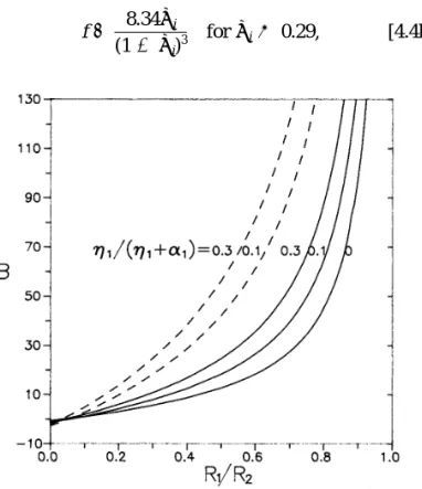
FIG. 2. The parameter B for a translating polymer-coated sphere situ-FIG. 1. The parameter B for a translating polymer-coated sphere

situ-ated at the center of a bare spherical cavity as a function of R1/R2with b10 ated at the center of a bare spherical cavity as a function of R1/R2. The

solid curves are plotted for the case of b10Å 10, and the dashed curves

Å100 in the free-draining limit ( fÅ1). The solid curves are plotted for

the case of aÅ0.5, and the dashed curves are plotted for the case of aÅ are plotted for the case of b10Å100. Note that d1/ar ` represents the

free-draining limit ( fÅ1). 0.25.

(10)

TABLE 2

Numerical Results of A/A`and B for a Rotating Polymer-Coated Sphere Situated at the Center of a Spherical Cavity

with Various Values of Parameters R1/R2and b10for Systems with No Polymer Tails in the Free-Draining Limit B A/A` b10Å10 b10Å100 b10Å1000 R1/R2 b2Å0 b2Åb1 b2Å0 b2Åb1 b2Å0 b2Åb1 b2Å0 b2Åb1 0 1.000 1.000 0.000 0.000 0.000 0.000 0.000 0.000 0.1 1.001 1.001 0.007 0.008 0.012 0.014 0.016 0.020 0.2 1.008 1.010 0.056 0.080 0.093 0.134 0.130 0.187 0.3 1.028 1.036 0.192 0.321 0.320 0.536 0.447 0.750 0.4 1.068 1.096 0.473 0.903 0.788 1.505 1.103 2.107 0.5 1.143 1.214 0.988 2.092 1.646 3.485 2.303 4.878 0.6 1.276 1.441 1.905 4.317 3.174 7.192 4.442 10.07 0.7 1.522 1.888 3.610 8.412 6.014 14.02 8.418 19.62 0.8 2.049 2.889 7.254 16.67 12.09 27.78 16.92 38.89 0.9 3.690 6.111 18.60 40.54 30.99 67.55 43.38 94.55 0.95 7.011 12.72 41.56 87.10 69.25 145.1 96.93 203.1 0.99 33.67 66.01 225.9 456.2 376.3 760.1 526.8 1064

boundary effect on B is increased when the value of d1/a free-draining limit are plotted for typical values of h1/(h1/

a1). Again, it is shown that the increase of the segment

is decreased for a given value of b10, the hydrodynamic

interactions among the polymer segments produce relatively fraction in the tails or the relative length of the tails increases the boundary effect on parameter B.

small effects on B.

We have also calculated parameter B for various cases of rotation of a spherical particle in a spherical cavity consider-4.2. Rotation of a Particle in a Cavity

ing the hydrodynamic interactions among the polymer seg-ments. In general, the differences between these calculations For the steady rotational motion of a spherical particle in

a concentric spherical cavity, results of A/A` and B (B` Å and the free-draining results are rather small.

0 in this situation) for various values of b10 and R1/R2 are

presented in Table 2 for systems with no tails in the free-draining limit. The value of A` for each case of b10 is the

same as that listed in Table 1. It is understood that the data of A/A` in Table 2 are also valid for situations with the

hydrodynamic interactions among the polymer segments. Similar to the case of translation of the particle, the ratio A/A`is independent of b10and it is a monotonic increasing

function of R1/R2. The value of B increases monotonically

with the increase of R1/R2 or b10. Also, the cavity with an

adsorbed polymer layer on its inside wall exerts more drag on the rotating particle than does a bare cavity if all the other conditions are constant. A comparison between Tables 1 and 2 shows that the boundary effect on the rotation of a polymer-coated particle, while can be quite significant, is much weaker than the boundary effect on the translation of the particle.

To consider the effect of tails in the adsorbed polymer layer surrounding the particle, we have also solved Eqs. [3.8], [3.9], and [3.16] for F*11 and F*12 over a range of h1

FIG. 3. The parameter B for a rotating polymer-coated sphere situated at

and a1for the case of a bare cavity. The ratio A/A` is inde- _{the center of a bare spherical cavity as a function of R}₁_/R₂_{with b}₁₀_Å_{100 in}

pendent of the parameter h1/(h1/ a1) or a1. In Fig. 3, the the free-draining limit ( fÅ1). The solid curves are plotted for the case of a

Å0.5, and the dashed curves are plotted for the case of aÅ0.25.

(11)

5. CONCLUDING REMARKS

The translational and rotational motion of a spherical par-ticle coated with a layer of adsorbed polymers in a concentric spherical cavity has been analyzed in this work. The inside wall of the cavity may also be covered by an adsorbed poly-mer layer. The analysis provides simple equations which must be solved, given the polymer segment density distribu-tions r(yi) and rheological parameters m(yi) and bi(yi), to

determine the parameters A and B of Eq. [2.9]. The hydrody-namic force and torque exerted on the particle, which is correct to O(l2

1), can be calculated using Eqs. [2.8] and [3.2]

and the results of A and B. For the exponential polymer segment distribution given by Eq. [4.1], the ratio A/A` is

found to be independent of the values of b10, d1/a, a1, and

h1/(h1/a1), and its results for various values of R1/R2are

listed in Tables 1 and 2. The dependence of B on b10, d1/a,

a1, h1/(h1 /a1), and R1/R2 is given in Tables 1 and 2 and

Figs. 1 – 3. The results indicate that the boundary effects on

FIG. 5. The parameter B for a translating polymer-coated sphere

situ-the motion of a polymer-coated particle can be significant. _{ated at the center of a spherical cavity as a function of R}

1/R2with the Throughout the calculations in the previous section we segment density distributions given by Eq. [5.2] and b10Å100 in the

free-draining limit. The dashed curves are plotted for the case of a bare cavity

have assumed a simple exponential decay of the polymer

(b2Å 0), and the solid curves are plotted for the case of b2Åb1. The segment density. This could be an oversimplification since

corresponding results for the exponential segment distribution are also

plot-the convex and concave nature of plot-the surfaces of plot-the particle

ted for comparison.

and the cavity wall might adjust the excluded volume effects among the polymer segments. A segment density of the

following form allows for curvature effects on polymer dis- _{r( y}

i) Åri0

e0y_i/d_i

1/(302i)s( yi/Ri)

i Å1 or 2, [5.1] tribution:

where s should be a positive value. For systems with no tails in the free-draining limit, bi(yi) has the form of the above

equation with ri0replaced by bi0. It is understood that

param-eters A` and A are independent of the curvature coefficient

s. We have numerically solved Eqs. [2.26] and [2.27] with the segment distribution given by Eq. [5.1] and substituted the solution of Giand Hiinto Eq. [2.28b] to compute

parame-ter B. These calculations, which are plotted in Fig. 4, indicate that the value of B decreases with the increase of s for various values of R1/R2as one would expect.

One may wish to consider a polymer segment distribution that is uniform over a distance from the solid surfaces:

r( yi) Åri0 if 0 £yi£di, [5.2a]

r( yi)Å 0 if yiú di. [5.2b]

For this profile in the free-draining limit, bi(yi) has the form

of Eq. [5.2] with ri0 replaced by bi0 and it can be shown

that

FIG. 4. The parameter B for a translating polymer-coated sphere situ-ated at the center of a spherical cavity as a function of R1/R2with the

A_` Å10b01/2

10 tanh b 1/2

10, [5.3a]

segment density distributions given by Eq. [5.1] and b10Å100 in the

free-draining limit. The dashed curves are plotted for the case of a bare cavity

(b2Å0), and the solid curves are plotted for the case of d2Åd1and b20 B

` Å 0 1

A`b10

(10sech b1/2

10)2. [5.3b]

(12)

Equation [5.3a] was obtained by Anderson and Kim (21), R2 radius of the spherical cavity (m)

s curvature coefficient defined by Eq. [5.1]

and it can be found that the value of A` is about six times

greater (if b10 É 100) for an exponential distribution of Td torque exerted by the fluid on the particle

(N m) segments than for the polymer uniformly distributed over a

region of thickness d1. Although A`is a function of b10for U translational velocity of the particle (m/s)

v_J(O)

fluid velocity in the outer region (m/s) this segment distribution, the ratio A/A` is independent of

the segment distribution and its results for the cases of b2 vJ(I)i fluid velocities in the inner regions (m/s) Å0 and b2Åb1have been given in Tables 1 and 2. In Fig. vJ(p) velocity of polymer segments (m/s)

5, the numerical results of parameter B for a translating y1 l011 (r 0R1) (m)

polymer-coated sphere located at the center of a spherical y2 l

01

2 (R20r) (m)

cavity versus the ratio R1/R2obtained using Eq. [5.2] for the z axial coordinate (m)

segment distribution are plotted. The corresponding results ai ratio of loop-to-tail length scales for a

poly-for the case of an exponential distribution of segments are mer layer

also plotted in the same figure for comparison. It can be bi parameters defined by Eq. [2.4a]

seen that the boundary effect on B is much weaker for the bi0 parameters defined by Eq. [4.3]

uniform distribution of segments over a distance from the gi coefficients defined by Eq. [2.22]

solid surfaces than for the exponential distribution of seg- _g_*_i coefficients defined by Eq. [3.14]

ments. _d₁ _{length scale of the polymer layer}

sur-rounding the particle (m)

d2 length scale of the polymer layer adsorbed

APPENDIX: NOMENCLATURE

on the cavity wall (m)

z Stokes friction coefficient of a polymer

seg-a Stokes radius of a polymer segment (m)

ment (kg/s)

A, B parameters defined by Eq. [2.9]

hi fraction of tails as defined by Eq. [4.1]

A`, B` parameters defined by Eq. [2.29] or [3.17] _{u, f} _{angular spherical coordinates}

bi, ci, di coefficients defined by Eq. [2.23]

li di/Ri

coefficients defined by Eq. [3.15]

b*i, c*i, d*i _m _{viscosity inside a polymer layer (kg/m s)}

C, D, E, F coefficients defined by Eq. [2.10] (m3

, m, _m

s fluid viscosity (kg/m s)

0, m02

) _r _{polymer segment distribution (m}03

) Cn, Dn, En, Fn coefficients defined by Eq. [2.11] or [2.12] _r

i0 polymer segment density in loops at the

sur-(m3

, m,0, m02

) _{face (m}03

) e_Jf, eJz unit vectors in the f and z directions, re- _f

i (4/3)pa

3

r(yi)

spectively _f

i0 (4/3)pa3ri0

f parameter for the hydrodynamic interac- _C _{Stokes stream function (m}3

/s) tions among polymer segments defined _C(O)

stream function in the outer region (m3

/s)

by Eq. [2.1a] _{stream functions in the inner regions (m}3

/s)

C(I)

i

Fd hydrodynamic force exerted on the particle Ã _{variable defined by Eq. [2.13b]}

(N) _{angular velocity of the particle (s}01

)

V_J

Fin functions of yidefined by Eq. [2.15] (m2)

functions of yidefined by Eq. [3.7b] (m)

F*in

ACKNOWLEDGMENT

Gi, Hi functions of yidefined by Eq. [2.25] (m)

K wall correction factor defined by Eq. [2.8]

This work was supported by the National Science Council of the Republic

K* wall correction factor defined by Eq. [3.2] _{of China under Grant NSC 83-0402-E002-067.}

l R1/R2

L effective hydrodynamic thickness of the

REFERENCES

polymer layer defined by Eq. [2.8] or

[3.2] (m) 1. Silberberg, A., J. Phys. Chem. 66, 1872 (1962).

2. Hoeve, C. A. J., J. Chem. Phys. 44, 1505 (1966).

M, N coefficients defined by Eq. [3.3b] (m3

,0)

3. Dimarzio, E. A., and Rubin, R. J., J. Polym. Sci., Polym. Phys. Ed. 16,

Mn, Nn coefficients defined by Eq. [3.4] or [3.5]

457 (1978).

(m3

,0)

4. deGennes, P. G., Macromolecules 13, 1069 (1980).

p hydrodynamic pressure (N/m2

) _{5. Fuller, G. G., J. Polym. Sci., Polym. Phys. Ed. 21, 151 (1983).} r radial spherical coordinate (m) 6. Anderson, J. L., McKenzie, P. F., and Webber, R. M., Langmuir 7, 162

(1991).

(13)

7. Stromberg, R. R., Tutas, D. J., and Passaglia, E., J. Phys. Chem. 69, 18. Kawaguchi, M., and Takahashi, A., Adv. Colloid Interface Sci. 37, 219 (1992).

3955 (1965).

19. Varoqui, R., and Dejardin, P., J. Chem. Phys. 66, 4395 (1977). 8. Doroszkowski, A., and Lambourne, R., J. Colloid Interface Sci. 26,

20. Hatano, A., Polymer 25, 1198 (1984). 214 (1968).

21. Anderson, J. L., and Kim, J., J. Chem. Phys. 86, 5163 (1987). 9. Garvey, M. J., Tadros, Th. F., and Vincent, B., J. Colloid Interface Sci.

22. Cohen Stuart, M. A., Waajen, F. H. W. H., Cosgrove, T., Vincent, B., 55, 440 (1976).

and Crowley, T. L., Macromolecules 17, 1825 (1984). 10. Kato, T., Nakamura, K., Kawaguchi, M., and Takahashi, A., Polym. J.

23. Giddings, J. C., Kucera, E., Russell, C. P., and Myers, M. N., J. Phys. 13, 1037 (1981).

Chem. 72, 4397 (1968).

11. Kim, J. T., and Anderson, J. L., Ind. Eng. Chem. Res. 30, 1008 (1991).

24. Glandt, E. D., AIChE J. 27, 51 (1981). 12. Carvalho, B. L., Tong, P., Huang, J. S., Witten, T. A., and Fetters, L. J.,

25. Bungay, P. M., and Brenner, H., Int. J. Multiphase Flow 1, 25 (1973).

Macromolecules 26, 4632 (1993).

26. Happel, J., and Brenner, H., ‘‘Low Reynolds Number Hydrodynam-13. Napper, D. H., ‘‘Polymeric Stabilization of Colloidal Dispersions.’’ _{ics.’’ Martinus Nijhoff, Dordrecht, The Netherlands, 1983.}

Academic Press, London, 1983. _{27. Zydney, A. L., J. Colloid Interface Sci. 169, 476 (1995).} 14. Russel, W. B., Saville, D. A., and Schowalter, W. R., ‘‘Colloidal Dis- _{28. Keh, H. J., and Chiou, J. Y., AIChE J. 42, 1397 (1996).}

persions.’’ Cambridge University Press, London, 1989. _{29. Fleer, G. J., Cohen Stuart, M. A., Scheutjens, J. M. H. M., Cosgrove,} 15. Gramain, Ph., and Myard, Ph., Macromolecules 14, 180 (1981). T., and Vincent, B., ‘‘Polymers at Interfaces.’’ Chapman & Hall, Lon-16. McKenzie, P. F., Kapur, V., and Anderson, J. L., Colloids Surf. A 86, don, 1993.

263 (1994). 30. Gerald, C. F., and Wheatley, P. O., ‘‘Applied Numerical Analysis,’’ 5th ed. Addison-Wesley, Reading, MA 1994.