Antipodal Paraunitary Matrices and Their Application
to OFDM Systems
See-May Phoong, Senior Member, IEEE, and Kai-Yen Chang
Abstract—Paraunitary (PU) matrices and filterbanks have
played an important role in many applications. This paper studies a special class of PU matrices, called antipodal paraunitary (APU) matrices. APU matrices are PU matrices whose coefficient ma-trices consist of 1 only. Several new methods will be introduced for the construction of APU matrices. In particular, a new method based on the butterfly structure that has a low cost implementa-tion is proposed. Moreover, one applicaimplementa-tion of APU matrices in precoded orthogonal frequency division multiplexing (OFDM) systems will be considered. By using an APU precoding matrix, the complexity will be very low, and experiments show that the use of APU matrices can greatly enhance the performance.
Index Terms—Antipodal paraunitary matrices, filterbanks,
OFDM.
I. INTRODUCTION
M
ULTIRATE systems and filterbanks (FBs) have played an important role in various areas of signal processing [1]–[3]. They have been successfully applied to source coding and compression, subband adaptive filtering, denoising, multi-carrier communications, etc. Of particular interest is the class of paraunitary (PU) matrices and FBs. One attractive feature of these matrices is their energy preservation property that can avoid the noise or error amplification problem. In the past, the design and complete parameterization of PU matrices have been successfully derived [4], [5]. In this paper, we are going to study a special class of PU matrices and FBs, namely, antipodal pa-raunitary (APU) matrices and FBs. A PU matrix is said to be an APU matrix if all of its coefficient matrices have as their entries. For the special case of constant (memoryless) matrices, APU matrices reduce to the well-known Hadamard matrices. One of the attractive features of these matrices is its low imple-mentational cost; only additions are needed.APU matrices are closely related to the complementary se-quences (or more commonly known as the Golay sese-quences) [6] and the -shift cross-orthogonal sequences [7]–[10]. The applications of APU matrices and complementary sequences in areas of communications such as synchronous spread spectrum communications and code division multiple access (CDMA) systems have been explored in [11] and [12]. In the past, many construction methods for APU matrices have been proposed [7],
Manuscript received November 2, 2003; revised March 29, 2004. This work was supported by the National Science Council, Taiwan, R.O.C., under Grant NSC 93-2752-E-002-006-PAE and NSC 93-2213-E-002-103. The associate ed-itor coordinating the review of this manuscript and approving it for publication was Prof. Tulay Adali.
The authors are with the Department of Electrical Engineering and the Grad-uate Institute of Communication Engineering, National Taiwan University, Taipei, Taiwan, R.O.C. (e-mail: smp@cc.ee.ntu.edu.tw).
Digital Object Identifier 10.1109/TSP.2005.843735
[9], [11], [13], [14]. In [13] and [14], it is shown that we can con-struct 2 2 APU matrices by cascading 2 2 Hadamard ma-trices and diagonal mama-trices with delay elements. This method is extended for the construction of APU matrices in [11]. In [7], it was shown that given a pair of complementary sequences, we can construct 2 2 APU matrices. Moreover, it was shown that the corresponding time-domain sequences of the APU matrices and their 2-shifts form an orthogonal basis for the class of finite energy signals. In [9], several methods are pro-posed for the construction of APU matrices from APU matrices of smaller dimensions. Except for [11], most of these studies use the time domain approach, and there are relatively few systematic studies on the theory and construction methods of APU matrices.
In this paper, we apply the theory of PU matrices to the study of APU matrices. All the derivations will be done using a -do-main approach. This approach not only gives a compact descrip-tion of the previous results but also enables us to generalize pre-vious methods. In addition, several new construction methods are proposed. In particular, a new construction method based on the well-known butterfly structure is introduced. APU ma-trices constructed using the butterfly structure can be imple-mented efficiently and, hence, have very low cost. Existence issue of APU matrices will also be explored. Unlike PU ma-trices, there are some constraints on the degree, order, and di-mension of APU matrices. We also consider one potential appli-cation of APU matrices. OFDM systems with APU precoding matrices are studied. By choosing APU matrices as the pre-coding matrix, we can have very low complexity. Moreover, we are able to average the noise variance in both the time and fre-quency domains, and this achieves time and frefre-quency diver-sity. Both zero-forcing and MMSE receivers for the precoded OFDM systems will be derived. Simulation results show that precoded OFDM systems have a much better performance than the OFDM system.
The paper is organized as follows. In Section II, we first give some definitions and notations. Then, the connection between the orthogonal sequences and APU matrices will be reviewed in Section III. Some existing construction methods of APU ma-trices will be described in Section IV. A number of new con-struction methods will be introduced in Section V. The existence issue of APU matrices will be explored in Section VI. In Sec-tion VII, we study OFDM systems with APU precoding ma-trices. We will analyze the noise performance of these systems. Numerical experiments are provided in Section VIII to compare the performances of the precoded OFDM systems. Conclusions are given in Section IX. Parts of the results have been presented in conferences in [15] and [16].
II. DEFINITIONS ANDNOTATIONS
In this section, we will introduce some definitions and notations. These preliminaries not only make this paper more self-contained but also facilitate the development of a -domain framework later.
1) Antipodal Sequences and Polynomials: Sequences are
denoted as lowercase letters with index , such as . The discrete unit impulse is denoted by . It is equal to 1 when and otherwise. All sequences studied in this paper are finite impulse response (FIR). A causal sequence of length is said to be
an-tipodal (AP) if for and
0 otherwise. The -transforms of sequences are de-noted by the corresponding uppercase letters, such as . The -transform of an AP se-quence will be called an AP polynomial.
2) All vectors and matrices are represented by boldfaced letters. The symbols and are reserved for the iden-tity and permutation matrices, respectively. and denote the transpose and the transpose conjugate of , respectively. A constant matrix is said to be AP if all of its entries are .
3) A polynomial matrix will be denoted by . A
poly-nomial matrix is AP if are
AP for .
4) Order, Length, and Degree: Let
with both and .
Then the order and length of are, respectively, and . Its degree is the minimum number of delays needed to implement . For example, the order of is equal to 1, while its degree is equal to the rank of .
5) Tilde Notation: Given a polynomial matrix , its tilde is defined [1] as
For a polynomial matrix with real coefficients, .
6) Cross Correlation: Given two sequences and , their th cross correlation coefficient is given by
Using the tilde notation, the z-transform of the cross-correlation coefficients can be expressed as
7) Kronecker Product of Matrices: Given two square
polynomial matrices and with dimensions and respectively, their Kronecker product is defined as shown in the equation at the bottom of the
page. Note that is an
matrix. Moreover, if the orders of and are and , respectively, then the order of
will be . Note that when the matrices are constant matrices independent of , then the above definition reduces to the conventional Kronecker product. One can verify that the tilde of
is equal to . Let the dimensions of the
matrices , and be so that all
the matrix multiplications in the following expression are valid. Then, the product rule states that
(1) 8) Paraunitary and Normalized Paraunitary Matrices:
An polynomial matrix is said to be
paraunitary (PU) [1] if
(2) for some nonzero constant . When , we say that is a normalized PU matrix. The above relation implies that is unitary for all frequency . It is well known that normalized PU matrices enjoy the energy-preservation property [1]. That is, if the input of a normalized PU matrix is a vector sequence of finite energy, the output vector satisfies
(3) Using the product rule, one can show that given two PU matrices and (not necessarily of the same dimensions), their Kronecker product is also PU.
9) Hadamard Matrices: An Hadamard matrix, denoted by , is a constant AP matrix (independent
of ) that satisfies . It was shown
[17] that a necessary condition for the existence of a Hadamard matrix is that must be 2 or a multiple of 4. Whether this is also a sufficient condition is still not known. Most of these Hadamard matrices have been successfully constructed; see [8] and references therein.
10) Antipodal PU Matrices: If a PU matrix is also an-tipodal, then it is called an antipodal paraunitary (APU)
..
matrix. It is not difficult to verify that if an by
matrix is APU, then it
satis-fies , and its
in-verse is also APU.
III. CROSS-ORTHOGONALSEQUENCES ANDAPU MATRICES
In the following, we will first define three types of sequences that are widely used in communications and then describe the connection between APU matrices and these sequences.
1) A set of antipodal sequences of length , for , is said to be complementary [9] if
(4) When , the complementary sequences are also known as the Golay codes [6].
2) An antipodal sequence of length is called an -shift orthogonal sequence [7], [10] if
-shift orthogonal sequences are closely related to complementary sequences. To see this, let
. Then, one can verify that are com-plementary if and only if is -shift orthogonal. 3) A set of antipodal sequences
is called a set of -shift cross-orthogonal sequences [10] if i) each sequence is an -shift orthogonal sequences and ii) any pair of distinct sequences
and satisfies for all integers .
These sequences have been studied extensively in [6], [7], [9], and [10], and they have found many applications in communi-cations [10]–[12].
1) APU Matrices and M-Shift Orthogonal Sequences: The
sequences defined above are closely related to the APU ma-trices. From (2), we see that if an by matrix of length
is APU, then its entries satisfy
for
Note that the above expression is nothing but the z-do-main formulation of (4). Thus, the sequences for , on the th row of an APU matrix ,
are complementary for . Moreover, if we
use as the polyphase matrix of the analysis filterbank [1], then the analysis impulse responses satisfy
for . In other words, the impulse response is an -shift orthogonal sequence, and any two analysis filters form a pair of -shift cross-orthogonal sequences. Therefore, the study and construction of a set of -shift cross-orthogonal sequences are identical to those of the APU matrices. In the
following sections, we will see that FB theory not only greatly simplifies the derivations of many existing results but also leads us to some new construction methods for orthogonal sequences.
IV. -DOMAINAPPROACH TOEXISTINGCONSTRUCTION
METHODS OFAPU MATRICES
In the literature, a number of construction methods for APU matrices have been proposed. The earliest report dated back to 1969 when Taki et al. [7] successfully constructed 2 by 2 APU matrices using complementary sequences [6]. The by case was studied in [9] and [11]. In this section, we will review some existing construction methods of APU matrices. These results are mostly derived in the time domain in the orig-inal works. We will describe them using the -domain frame-work. The -transform approach not only greatly simplifies the derivation but also allows us to make comparisons with the pro-posed methods later on.
Before we illustrate the construction of APU matrices, we will state a simple result that is useful for the understanding of the following construction method. Let
and
be two AP polynomials. Then, it is clear that the following three polynomials
and (5) are AP polynomials. The lengths of the first two and the last two polynomials are and , respectively.
A. 2 by 2 APU Matrices
APU matrices that are 2 by 2 are closely related to comple-mentary sequences or, more commonly, Golay sequences [6], [7]. Recall from the previous section that a pair of AP sequences
and of length are complementary if they satisfy (6) It is well known [1] that given a pair of polynomials satisfying (6), we can form a two-channel PU filterbank by choosing the two analysis filters as
(7) Such a construction has been derived by Taki et al. in [7]. It was shown therein that even shifts of and form an orthogonal basis for the class of finite energy signals. Let be the analysis polyphase matrix
Using (6), it is straightforward to verify that . The matrix is APU. Hence, every pair of Golay sequences generates a 2 by 2 APU matrix. Golay sequences with length
(where are integers) have been success-fully constructed in [6]. No Golay sequence of other lengths has been found thus far.
Another construction method for 2 by 2 APU matrices with length equal to a power of two was discovered independently by Shapiro [13] and Rudin [14]. Their algorithm is defined recur-sively as follows. Let : the 2 2 Hadamard matrix. For , let be recursively defined as
where the diagonal matrix is
As , and are PU matrices, so is their
product [1]. It is not difficult to verify that are AP for all . Therefore, are APU matrices with length equal to .
B. APU Matrices
The idea of Golay sequences was generalized to comple-mentary sequences in [9]. Unlike the two-channel case, there is no known method to construct an -channel APU-FB from a set of complementary sequences. Thus, the construction methods for complementary sequences were not helpful in generating by APU matrices. Nevertheless, there are al-gorithms that can generate APU matrices from APU matrices of smaller dimensions or lower orders. In the following, we will introduce four known methods.
Let be a 2 2 APU matrix of length . Thus, . Using this 2 2 matrix as a starting point, we can recursively generate two different sets of APU matrices using the following interleaving and concatenating methods.
1) Tseng’s Interleaving Method [9]: For , let be the matrix defined by (8), shown at the bottom of the page.
2) Tseng’s Concatenating Method [9]: For , let be the matrix defined by (9), shown at the bottom of the page. One can verify by direct multiplication that . Hence, defined in the above two equations are PU matrices. Moreover, using (5), it is not difficult to see that are AP of length . Therefore, the interleaving and concatenating methods generate APU matrices. One can generalize the two methods by choosing
as any by APU matrix with length . It is not difficult to show that in this case, the two methods will generate
by APU matrices with length .
3) Tseng’s Kronecker Product Method [9]1: Let be an
by APU matrix of length . Let be an integer for which an by Hadamard matrix exists. Consider the
fol-lowing by matrix
(10) Recall that the Kronecker product of two PU matrices is also PU. The AP property of the above matrix can be easily verified using the definition of Kronecker product. Thus, the matrix defined in (10) is an APU matrix of length .
4) Wornell’s Method: In [11], Wornell generalized the
Shapiro-Rudin construction method to the -channel case. Let be an integer for which Hadamard matrix exists. Let be the diagonal matrix:
..
. ... . .. ...
Let . Then, the algorithm can be described as [11]
(11) for . It is not difficult to verify that the above algorithm generates APU matrices of length .
V. NEWCONSTRUCTIONMETHODS FORAPU MATRICES
In the following, we present three new construction methods for APU matrices. The first two methods are simple gen-eralizations of Tseng’s Kronecker product method and the Agayan–Sarukhanyan theorem [8]. The last construction method is based on the butterfly structure.
1) Generalized Kronecker Product Method: Let and be APU matrices of dimensions and , respectively. Let and be their respective lengths. Consider the fol-lowing two matrices:
(12) (13) 1Alhough it was described differently in [9], we have chosen to express the
results in a Kronecker product form as it gives a far more compact expression.
(8)
Using the fact that the Kronecker product of two PU matrices is also PU, one can see that the above two matrices are PU. The AP property of these matrices follows directly from (5). Hence, the two formulas in (12) and (13) generate two APU ma-trices with length and dimension . When
, (13) reduces to Tseng’s Kronecker product method. The above two seemingly simple generalizations of Tseng’s Kro-necker product method also include Tseng’s interleaving and concatenating methods as special cases. To see this, let
and
Then, one can verify that (12) and (13) reduce, respectively, to Tseng’s interleaving method in (8) and Tseng’s concatenating method in (9).
2) Generalized Agayan–Sarukhanyan (AS) Method: Using
the multiplication theorem of Agayan–Sarukhanyan (AS) [8], it was shown that given two Hadamard matrices of dimensions and , one can construct a Hadamard matrix of dimension . We now show that the result can be generalized to the case of APU matrices. Let and be APU matrices of dimensions and , respectively. Suppose that their lengths are and , respectively. Consider the following partitions:
where and are and
matrices, respectively. This partition is always possible as and are even (see next section for a proof). Form
the following matrix with length
(14) where the submatrices are given by
The matrix , formed in such a manner, is called the AS multiplication2of and , which are denoted as
It is proved in the Appendix that the matrix is an APU ma-trix. Similarly, one can show that is also an APU matrix with length . Let be such that Hadamard matrices of dimension exist. Then, we can apply the generalized AS multiplication to
gen-erate by APU matrices of length (where
are integers). To see this, let be a 2 by 2 APU ma-trix with length . Such an APU matrix can be obtained from Golay sequences (see Section IV-A). Then, the following matrix
is an by APU matrix of length . Comparing our results with the Wornell’s method in (11), we see that the matrices con-structed using (11) have length equal to , whereas our ma-trices have length equal to .
3) Butterfly Structure Method: Let be an integer for which an Hadamard matrix exists. Define the fol-lowing two matrices:
(15)
Let and be an Hadamard matrix . Then,
the following iterative procedure generates two classes of APU matrices:
(16) where are arbitrary permutation matrices. Because of the delays in , the AP property is preserved. More-over, is PU because it is a product of PU matrices. Hence, is APU, and its length is . Similarly, one can show that is also APU with length . For example, Fig. 1 shows for and . Note that the butterfly structure has the additional advantage of low complexity. Its computa-tional cost for adding one stage is additions. When is a power of two, the Hadamard matrix can also be re-alized using the butterfly structure [19]. This gives rise to an efficient implementation of APU matrices. Given an
APU matrix of length , roughly additions are needed in direct implementation. If both and are powers of 2 and the APU matrix is constructed using the butterfly structure, then
only additions are needed.
4) Connection Between the Butterfly Structure Method and Wornell’s Method [11]: When the number of channels is a power of two, we can show that the butterfly structure method 2The original multiplication is defined for constant matrices independent of
Fig. 1. An 8 by 8 APU matrix with length 4 constructed using the butterfly method.
Fig. 2. (a) Efficient implementation of the 8 by 8 Hadamard matrixH 3(z). (b) Equivalent system.
includes Wornell’s method [11] as a special case. We demon-strate this for the case of . To do this, we need to show that in (11) can be expressed a product of matrices of the form , as in (16). It is well known [19] that the 8 8 Hadamard matrix can be implemented efficiently using butter-flies. Using the butterfly structure, we can implement
as Fig. 2(a). After moving some delay elements to the right of the butterflies, we can redraw Fig. 2(a) as Fig. 2(b). Note that the three stages (indicated by the dotted boxes) in Fig. 2(b)
can be, respectively, described as and
by choosing the permutation matrices properly. We summarize the different methods to obtain APU matrices in Table I. The possible dimensions and lengths of APU matrices generated from different methods are listed. The inter-leaving and concatenating methods, the generalized Kronecker product method, and the generalized AS method construct APU matrices from APU matrices of smaller dimensions. In each it-eration, both the length and dimension of resulting APU ma-trices might increase. On the other hand, the Shapiro and Rudin method, the Wornell method, and the butterfly method can be used for APU matrices of a fixed dimension. Only the length of APU matrices increases in each iteration.
5) Comments:
1) Note that pre- or post-multiplying an APU matrix with either a permutation matrix or a diagonal matrix with all diagonal entries equal to generates another APU matrix.
TABLE I
SUMMARY OFDIFFERENTMETHODS TOGENERATEAPU MATRICESWITH
DIMENSIONMANDLENGTHN. THENUMBERSM ANDN AREINTEGERS FORWHICHAPU MATRICES OFDIMENSIONSM ANDLENGTHN EXIST
2) Except for the generalized AS multiplication, all the construction methods in the previous two sections can be modified so that they can be used to generate com-plex PU matrices with unit-magnitude coefficients. For example, if the Hadamard matrix in (10) or (11) is replaced by a unitary matrix with unit-magnitude en-tries (the discrete Fourier transform (DFT) matrix is a matrix with such a property), then (10) or (11) will generate complex PU matrices with unit magnitude co-efficients. For any integer , we know that an by DFT matrix exists. Hence, we can generate by complex PU matrices with unit-magnitude coeffi-cients for any .
6) APU Matrices and Block Circulant Hadamard Ma-trices: Let be an APU matrix with length .
That is, . Then, using the time domain
expression of , one can verify by direct
multiplication that the following matrix is a Hadamard matrix:
..
. ... . .. ... (17)
The above Hadamard matrix has a block circulant structure. Thus, given any APU matrix, we can construct a block circu-lant Hadamard matrix.
7) Rectangular APU Matrices: One can extend the
defini-tion of APU matrices to include rectangular matrices. A
matrix is APU if all of entries of
are , and it satisfies . Clearly, we have . It is not difficult to verify that we can obtain rectan-gular APU matrices by deleting some columns of square APU matrices. Many previously described methods can be easily ex-tended to derive rectangular APU matrices. For example, if we take to be a rectangular submatrix formed by deleting some columns of a Hadamard matrix, then the interleaving and concatenating methods, the Wornell method, and the butterfly method will generate rectangular APU matrices.
VI. EXISTENCEISSUES OFAPU MATRICES
It is known that Hadamard matrices exist only when the di-mension is 2 or a multiple of 4 [17]. Whether this is also a suffi-cient condition is still unknown, but so far, no counter example has been found. In this section, we will study similar issues for
APU matrices. We will first study the case of first-order APU matrices. Then, results for the more general case will be dis-cussed.
Consider the first-order APU matrix:
(18) Such a matrix is also known as a lapped transform. Applying the PU conditions in (2) to the matrix , we can obtain the following four conditions:
(19) (20) (21) (22) As both and are AP matrices, one can immediately con-clude from (19) or (20) that the dimension is even. From FB theory, it is well known [1] that all PU matrices can be minimally realized as a cascade of simple degree-one PU matrices. For the case of APU matrices, such simple degree-one APU building blocks do not exist (except for the special case of ). This is a direct consequence of the following theorem.
Theorem 1: Let be an APU
matrix. Then, rank rank .
Proof: Let rank . From the factorization theorem of PU matrices [1], we know that
(23)
for some matrix satisfying . By direct
substitution, one can verify that the matrix . Using (19) and (21), we get . Multiplying both sides of (23) by and comparing the coefficient of
, we obtain
Since , we have
trace trace trace
As trace and , we get ,
which implies . From (23), we get rank .
From the above theorem, we see that the degree of an first-order APU matrix is . Thus, except for , we cannot have a degree-one APU building block.
Although the existence issue of Hadamard matrices has been studied extensively (see [8] and references therein), there are essentially no reports on the existence issue of the APU ma-trices. From Wornell’s method [11] and the butterfly method, we know that we can construct APU matrices from Hadamard matrices of the same dimension. Hence, we can immediately conclude that if is 2 or a multiple of 4, APU matrices of higher order exist. However, since APU matrices are more gen-eral than Hadamard matrices in the sense that they have more
free parameters, whether this is a necessary condition for the existence of APU matrices is still unknown. However, we are able to obtain a number of results listed below. Let
be an APU matrix.
Then, we have the following.
• The number is even. This can be verified from the facts that and are AP matrices satisfying
.
• If is odd, then is a multiple of 4. To see this, recall from (17) that we can have an
Hadamard matrix from . As Hadamard matrices exist only for dimension equal to 2 or a multiple of 4, if is an odd integer other than 1, then has to be a multiple of 4.
• There does not exist any 2 2 APU matrix with odd . Otherwise, we could have constructed Hadamard matrices using (17), which is a contra-diction.
There are a number of open problems. For example, it is still unclear if there exist APU matrices with odd length . All the above construction methods generate APU matrices of even length only. In addition, we do not know if there are APU ma-trices with dimensions of , for .
VII. OFDM SYSTEMSWITHAPU PRECODINGMATRIX
Linearly precoded OFDM systems have been studied by a number of researchers [20]–[22]. Of particular interest is the OFDM system with a DFT precoding matrix. Such a system was shown to be the same as the so-called single carrier with frequency domain equalizer (SC-FDE) system [23]. In [20], it was shown that the SC-FDE system has the maximum diversity gain among all linearly precoded OFDM systems. In [21], a bit error rate (BER) minimized precoder for an OFDM system was considered. For high SNR transmission, the SC-FDE system is optimal in the sense that it minimizes the bit error rate among OFDM systems with any orthogonal precoding matrix. In these studies, the precoders are constant matrices independent of . In this section, we will study precoded OFDM systems with APU precoding matrices.
Fig. 3 shows the block diagram of a precoded OFDM system. In a precoded OFDM transmitter, the th input block , con-sisting of modulation symbols such as QAM symbols, is first passed through an by precoding matrix . The output of is given by
(24)
In this section, the precoding matrix is chosen as a
nor-malized APU matrix so that
That means that all the entries are scaled by . In prac-tice, this normalization constant can be absorbed into the signal power of modulation symbols. After taking the -point inverse
Fig. 3. OFDM system with APU precoding matrixT(z).
discrete Fourier transform (IDFT) of the vector , we get the vector
where is the DFT matrix with
. Note that unlike the conventional block trans-mission system, the transmitted block contains
informa-tion of the input blocks . Before
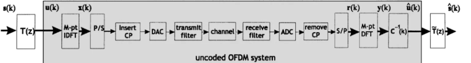
is transmitted, a cyclic prefix (CP) of length is added. In this paper, we assume that the channel is slowly varying so that for each OFDM block, the channel response does not vary. We model the combined effect of the digital-to-analog converter (DAC), transmit filter, channel, receive filter, and analog-to-digital converter (ADC) as an equivalent discrete time system with denoting the th tap of the impulse response when the th block is sent. We also assume that the CP length is large enough so that the length of the equivalent
channel is , that is, for all whenever
. The channel noise is assumed to be addi-tive white Gaussian noise (AWGN) with variance . At the receiver end, to remove the interblock interference, the first L samples of the received block that correspond to the cyclic prefix are discarded. We obtain the vector . Taking the DFT of , we get
(25) where is an diagonal matrix whose th entry is given by the DFT coefficient of the channel impulse response
(26)
The noise vector is an AWGN vector. Assume that the channel does not have spectral null so that is invertible. After multiplying the diagonal matrix , we get
(27) In the absence of channel noise, the vector for all . When the precoding matrix is PU, we can get a zero forcing receiver by taking as the decoding matrix,3as in-dicated in Fig. 3. Note that when we take
, the system in Fig. 3 reduces to the conventional uncoded OFDM system. It should be emphasized that even though the 3For convenience, we use a noncausal decoding matrix. A causal receiver can
be easily obtained by cascading enough delays.
precoded OFDM system has an overlapping-block transmitter, the channel impulse response can be different for dif-ferent block indices , and the system in Fig. 3 still has the zero-forcing property.
A. Noise Analysis
Define as
The autocorrelation matrices of are given by
(28) where is the variance of the channel noise . Because are diagonal matrices, we see from the above equation that is also an AWGN vector, but each entry has a different variance.
Define the output noise vector . Then, it can be viewed as the output of with the input vector . Therefore, we can write
Using the facts that is an AWGN vector and is a nor-malized PU matrix, one can verify that its zeroth autocorrelation matrix at the th block is given by
where is the zeroth autocorrelation matrix of given in (28). Note that is a diagonal matrix. Looking at the th diagonal term of , we can write the noise variance at th subband (when the th block is being processed) as
(29) where we have used (28) and the fact that all the entries of
have magnitude equal to . The quantity
is independent of ; all subbands have the same noise variance! Moreover, the decoding matrix has an averaging effect on the channel gains over a time period of blocks. Note that we make no assumptions about the APU matrix . Any APU precoding matrix can achieve (29). From (29), we also see that
Fig. 4. (a) Precoded OFDM system with an MMSE receiver. (b) Equivalent system.
the performance of precoded OFDM with a zero-forcing re-ceiver degrades significantly when one or some of the channel gains are small. The noise variances in all subbands will be very large over a period of blocks. To solve this problem, a min-imum mean-square-error (MMSE) receiver is needed and will be derived in the next subsection.
1) Comparison With the Uncoded OFDM and SC-FDE Sys-tems: When we take , the system in Fig. 3 be-comes the conventional uncoded OFDM system. In this case, . Thus, for an uncoded OFDM system, we can ob-tain from (27) the output noise variance at the th subband as
(30) The average output noise variance is
(31)
From (30), we see that depends on both and , and it is inversely proportional to . Recall that is the channel gain at the th frequency bin when the th block is sent. For highly frequency selective channels, some of the gains can be close to zero, and the performance of the OFDM system will be affected by these spectral nulls.
If we allow the definition of APU matrices to include complex matrices whose coefficients have unit magnitude, then the DFT matrix is APU. When we take , the system in Fig. 3 becomes the SC-FDE system [21]. By carrying out the same derivation, one can show that the noise variance of the SC-FDE system can be obtained by simply setting in (29). The noise variance at the th subband when the th block is sent is given by
(32)
Observe from the above expression that is independent of . All the subbands have the same noise variance, and they are equal to the average noise variance in (31).
We can clearly see the difference between the conventional OFDM, the SC-FDE and the APU-precoded OFDM systems
from the three expressions in (30), (32), and (29), respectively. Because the decoding matrices (for precoded OFDM system) and (for SC-FDE system) are PU, they have the energy (or power) conservation property [1]. The average output noise variance for the three systems is the same. However, they distribute these noise variances to the subbands differently. For the conventional OFDM system, each subband can have a very different noise variance, especially when the channel is highly frequency selective. From (30), we see that subbands having small will suffer from large noise variances. On the other hand, the SC-FDE system has an averaging effect in frequency domain; it averages over all subbands. When the channel has spectral nulls, all subbands will have large noise variances. To avoid this problem, an MMSE receiver is needed. Even when the channel does not have spectral nulls, for fast fading channel, the channel gains can vary rapidly with respect to . From (32), we see that if is small for some , the whole th block will be severely affected by noise amplification problem. The APU-precoded OFDM system has an averaging effect in both the frequency and time domains; it averages over all subbands and over OFDM blocks. Sim-ilarly, if the channel has spectral nulls, all the subbands will have large noise variances for the next transmission blocks. Hence, an MMSE receiver is needed for the OFDM system with APU precoding matrices.
B. MMSE Receiver for Precoded OFDM Systems
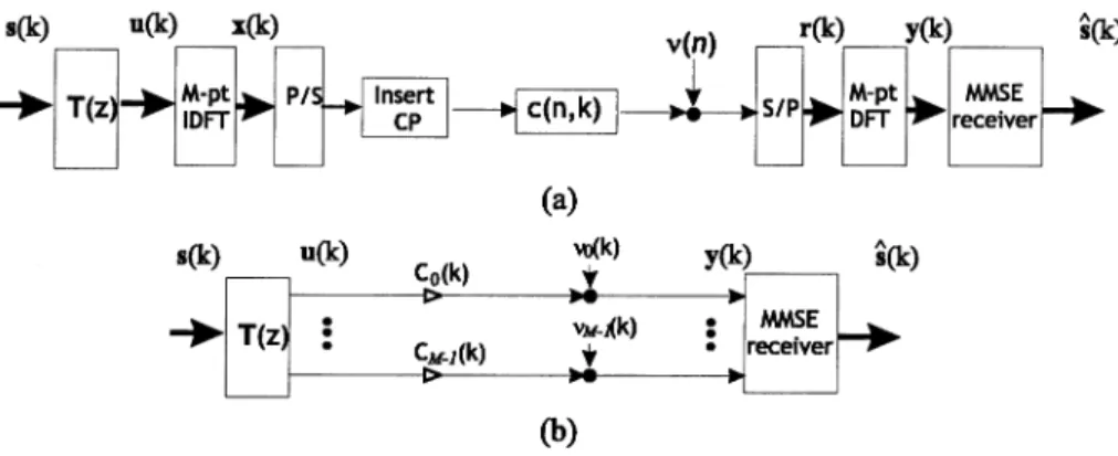
We assume that the receiver removes the first samples cor-responding to the cyclic prefix so that there is no interblock in-terference. Given the received vector , we want to design an MMSE receiver. As the DFT matrix is invertible, there is no loss of generality if we consider the system in Fig. 4(a). It is known that when the length of the channel length is , the frequency-selective channel is converted into a set of parallel nonfrequency-selective subchannels. We can redraw the system in Fig. 4(a) as Fig. 4(b), where is a diagonal ma-trix whose th entry is the th DFT coefficient of , as defined in (26). The equivalent noise is the AWGN vector with the power spectral matrix . In the following deriva-tions, we assume that the transmitted signals satisfy
In other words, the symbols are uncorrelated and have equal signal power. The fact that is normalized PU implies that
also satisfies
(34) Moreover, we also assume that the transmitted signals are un-correlated to the channel noise.
Consider an MMSE receiver (possibly time-varying) with coefficient matrices for . Given the input vector , the output of the MMSE receiver can be described as
(35)
where are matrices. For convenience, we con-sider the noncausal system. Our goal is to find so that the following mean square error is minimized:
Applying the orthogonality principle, one can show that the MMSE solution is given by (see the Appendix for a proof)
(36)
where . Note that
is a diagonal matrix whose th diagonal entry is given by
From the above expressions, we see that the MMSE receiver can be decomposed into a time-varying diagonal matrix and the time-invariant matrix . Therefore, we can implement the MMSE receiver as Fig. 5. Comparing the zero-forcing and MMSE receivers in Figs. 3 and 5, respectively, one immediately sees that their only difference is the one-tap equalizer. When there is no noise, i.e., , the MMSE receiver reduces to the zero-forcing receiver.
One can verify that for the precoded OFDM system with an MMSE receiver, all the subbands also have the same error vari-ance, and it is given by
(37)
One can clearly see from the above expression that the decoding matrix has an averaging effect in both frequency and time domains; it averages over all subbands and over OFDM blocks. Moreover, the quantities are upper bounded by . When some of the channel gains approach zero, the error variance does not go to infinity. We will see in the next section that by using an MMSE receiver,
Fig. 5. Implementation of the MMSE receiver.
the performance of the precoded OFDM system is improved significantly.
1) Precoders With Missing Powers in : From (37), we see that when the channel gains are slow-varying and remain virtually the same for blocks, then averaging effect becomes negligible, as we will see in the next section. One can increase the length of the precoder so that more terms are averaged, but this will increase the computational complexity. To avoid this, one can perform averaging over nonconservative blocks. To do this, we can use precoders with missing powers in . Let be an APU matrix. Then, for integer is also APU. Using as a precoder, the output error variance of all subbands becomes
Compared with , we need only extra delays to implement , and the computational complexity remains the same.
2) Choice of APU Matrices: As we have mentioned above,
given the length and dimension of the precoding matrix, all APU matrices have the same noise property. In practice, one can consider other criteria when choosing the APU matrices. For example, one can consider the peak-to-average power ratio (PAPR). It is well-known that OFDM system suffers from high PAPR. The PAPR of an -channel OFDM system is propor-tional to . For OFDM systems with an APU precoding matrix, one can choose the APU matrix to alleviate the PAPR problem. To see this, we can use a complex APU matrix of the form
(38) where is the by DFT matrix, and and are the by matrices defined in (15). The length of is . Consider Fig. 3. Because , the transfer matrix from the input vector , consisting of transmitted symbols, to is
Note that there are only stages of butterfly. The PAPR is at most for each stage. Hence, the PAPR is at most , which is equal to . In practice, is usually much smaller than . One additional advantage of using the APU matrix of the form in (38) is that there is no need to implement both the IDFT matrix and the DFT matrix at the trans-mitter. This leads to an additional computational saving. An-other possible criterion that can be incorporated into the design
Fig. 6. Bit error rate performance for slowly varying channels.
of APU matrices is the frequency response of the transmit fil-ters. This problem is beyond the scope of this paper.
VIII. SIMULATION
In this section, we carry out Monte Carlo experiments to verify the performance of precoded OFDM systems with dif-ferent precoders. The transmission channels are the modified Jakes fading channels described in [24]. In the experiments, we will use channel models with two different ratios of doppler fre-quency over transmission bandwidth. A larger value of indi-cates that the channel is changing faster. The ratio
corresponds to a slowly varying channel, whereas
corresponds to a channel that varies ten times faster. The number of taps of the channels is 16. The channel noise is AWGN with variance . In our simulation, we assume that the receiver knows the exact channel response. The DFT size is , and the length of cyclic prefix is . The input vector consists of quadrature phase shift keying (QPSK) symbols with power equal to .
APU matrices of different length will be used as the pre-coding matrices. When , the APU matrix reduces to the Hadamard matrix. It is known [21] that the OFDM system with a Hadamard precoding matrix has the same BER perfor-mance as the SC-FDE system. We plot the BER curves versus the signal-to-noise ratio (SNR), which is equal to . In the simulation, we do not consider the MMSE receiver for the conventional OFDM system because the BER performance of OFDM systems with MMSE receivers is identical to that of OFDM systems with zero-forcing receivers.
The results for are shown in Fig. 6. From the figure, we see that the performance of precoded OFDM system with a zero-forcing receiver is worse than that of the OFDM system at low SNR. This is because when the transmission en-counters deep fading at some frequency bins, all the outputs of precoded OFDM receiver will be seriously affected by channel noise. On the other hand, for the OFDM system, only a por-tion of the outputs will be seriously affected. However, when an MMSE receiver is employed, the precoded OFDM systems
Fig. 7. Bit error rate performance for fast varying channels.
have a much better performance than the OFDM system. If we compare the performance of precoded OFDM systems with dif-ferent precoders, we see that when the channel is slowly varying, using a longer precoding matrix does not provide much gain in performance. This is because when the channel variation in the time domain is small, averaging the performance in the time do-main has little effect on the performance.
For channel that is varying ten times faster with , the results are shown in Fig. 7. Again, we see that the precoded OFDM system with a zero-forcing receiver does not perform well, and using an MMSE receiver can greatly improve the per-formance of precoded OFDM systems. In addition, note that the performance improves as the length of the precoding matrix increases. As the channel is fast varying, averaging in the time domain can provide additional gain. If we compare the cases of and , averaging over eight blocks can yield an additional gain of more than 2 dB when the BER is .
IX. CONCLUSION
In this paper, a -domain approach is introduced to study APU matrices. This approach not only gives a compact descrip-tion of the previous results but also enables us to generalize previous methods. Moreover, several new methods for the con-struction of APU matrices have been introduced. In particular, APU matrices constructed by the butterfly method have the ad-ditional advantage of low implementational cost. We have also considered application of APU matrices in precoded OFDM systems. We have showed that by using an APU precoding ma-trix, the output noise is averaged in both time and frequency domain. Simulation results show that precoded OFDM systems with MMSE receivers have a significantly better performance than the conventional OFDM system.
APPENDIX
A. Proof of Generalized AS Method
In the following, we will show that the matrix is APU. Recall that the matrix
is given in (14). Define the two matrices
and .
Let and .
Then, one can verify that the entries of the coefficient ma-trices and consist of either or 0. Moreover, if , then and vice versa. Using this result, one can see from (14) that is antipodal. To show that is PU, we need to prove that
for some positive constant . In the following, we will show that
The proof for other terms is very similar. For notational com-plexity, we will drop the dependency on . Using the fact that
we can write
Using the product rule (1), one can write
Using the fact that for some positive , we can simplify the above equation as
Because for some positive , we can write
, which proves the result.
B. Derivation of the MMSE Receiver
Using the orthogonality principle, the MMSE receiver should satisfy
for (39)
From (25), (27), and (33), we immediately get
(40) Using (34), one can show that
Using the above result and (35), we have
(41) Substituting (40) and (41) into (39), we immediately get the result in (36).
ACKNOWLEDGMENT
The authors would like to thank Prof. S. C. Pei, National Taiwan University, Taipei, for bringing our attention to the results on Hadamard matrices with non power-of-two dimen-sions. They would also like to thank the anonymous reviewers and Prof. P. P. Vaidyanathan, Caltech, Pasadena, CA, for their constructive suggestions, which have significantly improved the manuscript.
REFERENCES
[1] P. P. Vaidyanathan, Multirate Systems and Filterbanks. Englewood Cliffs, NJ: Prentice-Hall, 1993.
[2] M. Vetterli and J. Kovacevic, Wavelets and Subband Coding. Engle-wood Cliffs, NJ: Prentice-Hall, 1995.
[3] G. Strang and T. Nguyen, Wavelets and Filterbanks. Wellesley, MA: Wellesley-Cambridge Press, 1996.
[4] M. J. T. Smith and T. P. Barnwell III, “A procedure for designing exact reconstruction filterbanks for tree-structured subband coders,” in Proc.
IEEE Int. Conf. Acoust. Speech, Signal Process., San Diego, CA, Mar.
1984, pp. 27.1.1–27.1.4.
[5] P. P. Vaidyanathan, “Theory and design ofM-channel maximally deci-mated quadraature mirror filters with arbitraryM, having perfect recon-struction property,” IEEE Trans. Acoust., Speech, Signal Process., vol. ASSP-35, pp. 476–492, Apr. 1987.
[6] M. J. E. Golay, “Complementary series,” IRE Trans. Inf. Theory, vol. IT-7, pp. 82–87, 1961.
[7] Y. Taki, H. Miyakawa, M. Hatori, and S. Namba, “Even-shift orthog-onal sequences,” IEEE Trans. Inf. Theory, vol. IT-15, pp. 295–300, Mar. 1969.
[8] J. Seberry and M. Yamada, “Hadamard matrices, sequences, and block designs,” in Contemporary Design Theory: A Collection of Surveys, J. H. Dinitz and D. R. Stinson, Eds. New York: Wiley, 1992.
[9] C.-C. Tseng and C. L. Liu, “Complementary sets of sequences,” IEEE
Trans. Inf. Theory, vol. IT-18, pp. 644–652, Sep. 1972.
[10] N. Suehiro and M. Hatori, “N-shift cross-orthogonal sequences,” IEEE
[11] G. W. Wornell, “Spread signature CDMA: Efficient multiuser commu-nication in the presence of fading,” IEEE Trans. Inf. Theory, vol. 41, no. 5, pp. 1418–1438, Sep. 1995.
[12] H. Chen, J. Yeh, and N. Suehiro, “A multicarrier CDMA architecture based on orthogonal complementary codes for new generations of wide-band wireless communications,” IEEE Commun. Mag., vol. 39, no. 10, pp. 126–135, Oct. 2001.
[13] H. S. Shapiro, “Extremal Problems for Polynomials and Power Series,” Master’s Thesis, Mass. Inst. Technol., Cambridge, MA, 1951. [14] W. Rudin, “Some theorems on Fourier coefficients,” in Proc. Amer.
Math. Soc., vol. 10, 1959, pp. 855–859.
[15] S. M. Phoong and Y. P. Lin, “Lapped Hadamard transforms and filter-banks,” in Proc. Int. Conf. Acoust. Speech, Signal Processing, Apr. 2003. [16] S. M. Phoong, K. Y. Chang, and Y. P. Lin, “Antipodal paraunitary pre-coding for OFDM application,” in Proc. Int. Symp. Circuits Systems, May 2004.
[17] R. E. A. C. Paley, “On orthogonal matrices,” J. Math. Phys., vol. 12, pp. 311–320, 1933.
[18] S. M. Phoong and P. P. Vaidyanathan, “Paraunitary filter banks over finite fields,” IEEE Trans. Signal Processing, vol. 45, no. 6, pp. 1443–1457, Jun. 1997.
[19] N. Ahmed and K. R. Rao, Orthogonal Transforms for Digital Signal
Processing. New York: Springer-Verlag, 1975.
[20] Z. Wang and G. B. Giannakis, “Linearly precoded or coded OFDM against wireless channel fades?,” in Proc. Third IEEE Workshop Signal
Process. Adv. Wireless Commun., Taoyuan, Taiwan, R.O.C., Mar. 2001.
[21] Y. P. Lin and S. M. Phoong, “BER minimized OFDM systems with channel independent precoders,” IEEE Trans. Signal Process., vol. 51, no. 9, pp. 2369–2380, Sept. 2003.
[22] Y. Ding, T. N. Davidson, Z.-Q. Luo, and K. M. Wong, “Minimum BER block precoders for zero-forcing equalization,” IEEE Trans. Signal
Process., vol. 51, no. 9, pp. 2410–2423, Sep. 2003.
[23] H. Sari, G. Karam, and I. Jeanclaude, Frequency-Domain Equalization
of Mobile Radio and Terrestrial Broadcast Channels. San Francisco, CA: Globecom, 1994.
[24] P. Dent, G. E. Bottomley, and T. Croft, “Jakes fading model revisited,”
Electron. Lett., pp. 1162–1163, Jun. 1993.
See-May Phoong (M’96–SM’04) was born in Johor,
Malaysia, in 1968. He received the B.S. degree in electrical engineering from the National Taiwan University (NTU), Taipei, Taiwan, R.O.C., in 1991 and the M.S. and Ph.D. degrees in electrical engi-neering from the California Institute of Technology (Caltech), Pasadena, in 1992 and 1996, respectively. He was with the Faculty of the Department of Elec-tronic and Electrical Engineering, Nanyang Techno-logical University, Singapore, from September 1996 to September 1997. In September 1997, he joined the Graduate Institute of Communication Engineering and the Department of Elec-trical Engineering, NTU, as an Assistant Professor, and since August 2001, he has been an Associate Professor.
Dr. Phoong is currently an Associate Editor for the IEEE SIGNALPROCESSING
LETTERS. He has previously served as an Associate Editor for the IEEE TRANSACTIONS ONCIRCUITS ANDSYSTEMSII: ANALOG ANDDIGITALSIGNAL
PROCESSINGfrom January 2002 to December 2003. His interests include mul-tirate signal processing, filterbanks, and their application to communications.
Dr. Phoong received the Charles H. Wilts Prize for outstanding independent research in electrical engineering at Caltech in 1997.
Kaiyen Chang was born in Taipei, Taiwan, R.O.C.,
in 1977. He received the B.S. degree in electrical engineering from the National Tsing Hua University (NTHU), Hsinchu, Taiwan, in 1999 and the M.S. degree in communication engineering from the National Taiwan University, Taipei, Taiwan, in 2003. His research focuses on the orthogonal frequency division multiplex systems.