Reduction Techniques for Training Support Vector Machines

Reduction Techniques for Training

Support Vector Machines

Kuan-ming Lin

Dept. Computer Science & Information Engineering National Taiwan University

• Reduced support vector machines (RSVM) analysis • RSVM implementations

• Performance of RSVM

• Study on incomplete Cholesky factorization (ICF) • Using ICF kernel approximation technique for SVM

(ICFSVM)

Support Vector Machines

• A promising method for data classifications

• Training and testing

• Training vectors : xi, i = 1, . . . , l

• Consider examples with two classes: yi =    1 if xi in class 1 −1 if xi in class 2

wT_{x + b = +1, 0, −1}

• Variables: w and b : Need to know coefficients of a plane • Decision function wTx + b, x: test data

SVM Formulation

• Maximize the margin _{2/kwk ≡ Minimize w}Tw/2 • Apply nonlinear mapping φ for training data

• Avoid overfitting for training data: allow training error ξ • A standard problem [Cortes and Vapnik, 1995]:

min w,b,ξ 1 2w T_{w + C} l X i=1 ξi yi(wTφ(xi) + b) ≥ 1 − ξi, ξi ≥ 0, i = 1, . . . , l

• w: a vector in an infinite dimensional space • Solve the SVM dual problem:

min α 1 2α T Qα − eTα 0 ≤ αi ≤ C, i = 1, . . . , l yTα = 0

e: vector of all ones, Qij = yiyjφ(xi)Tφ(xj).

Large-scale SVM Problems

• Q fully dense, cannot be saved in memory: traditional optimization methods not usable

• Decomposition methods: currently major approach

– iteratively solve smaller problems by fixing most variables

– slow convergence for huge problems with many support vectors

• Reduction techniques:

– alter the standard SVM formulation

– reduce the size of Q and solve the reduced problem • For how large problems is reduction better?

Performance not fully studied before

– testing accuracy: compare with standard SVM

The Reduced Support Vector Machine

• Proposed in [Lee and Mangasarian, 2001] • Start from a variant of SVM:

min w,b,ξ 1 2(w T_{w + b}2_{) + C} l X i=1 ξ_i2 yi(wTφ(xi) + b) ≥ 1 − ξi, i = 1, . . . , l

• Let w be Pl_i=1 αiyiφ(xi) (here α not dual variable):

min α,b,ξ 1 2(α T_{Qα + b}2_{) + C} l X i=1 ξ_i2 Qα + by ≥ e − ξ

• RSVM randomly selects a subset R of m samples as support vectors: w = P_i∈R αiyiφ(xi)

let ¯_{α ≡ α}R min ¯ α,b,ξ 1 2(¯α T_Q RRα + b¯ 2) + C l X i=1 ξ_i2 Q_{:,Rα + by ≥ e − ξ}¯ • Simplify 1/2¯αTQRRα to 1/2¯¯ αTα¯

• Absorb b by eQ ≡ hQ:,R y i , eα ≡  α¯ b   • The formulation of RSVM: min e α,ξ 1 2αe T e α + C l X i=1 ξ_i2 e Qeα ≥ e − ξ

• We find it similar to radical basis function networks – comparisons of RBF networks with SVM was done

• Smooth SVM (SSVM) in [Lee and Mangasarian, 2001] • Transform RSVM to an unconstrained problem:

min e α 1 2αe T e α + C Pl_{i=1((e − eQe}α)i)2₊

• (.)+ ≡ max(., 0) not differentiable

• Approximate (t)+ by Pβ(t) ≡ t + β−1 log(1 + exp(−βt)):

Differentiable, Newton’s method can be used

RSVM is Already in the Form of Linear SVM

• Linear SVM primal form: min w,ξ 1 2w T_{w + C} l X i=1 ξ_i2 Y Xw ≥ e − ξ • Formulation same with RSVM:

min e α,ξ 1 2αe T e α + C l X i=1 ξ_i2 e Qeα ≥ e − ξ

• Proposed in [Suykens and Vandewalle, 1999] – Change eQeα ≥ e − ξ to equality Qeeα = e − ξ • ξ is represented by eα: min e α f (eα) = 1 2αe T e α + C l X i=1 (e − eQeα)2_i

• Quadratic unconstrained, equivalent to a linear system: ( eQTQ +e I

2C )eα = eQ

Use Decomposition

• The dual form of RSVM:

min α 1 2α T_{( eQ eQ}T ₊ I 2C )α − e T_α 0 ≤ αi, i = 1, . . . , l – primal RSVM solution α = ee QTα

• Each iteration a working set of size q is to be modified • Main cost is calculating Q∆α: O(lqm) for O(m) kernel • Speedup for linear kernel and RSVM: Q∆α = eQ( eQT∆α)

O(mq) + O(lm) = O(lm) operations, q times faster • Used in software SV Mlight and BSVM

• Proposed in [Mangasarian and Musicant, 2001] • Consider optimality condition of dual RSVM:

Hα − e ≥ 0, α ≥ 0, (Hα − e)Tα = 0 with H ≡ eQ eQT + _2CI • Equivalent to Hα − e = (Hα − e − βα)+, ∀β > 0:

apply fixed-point iterations (each step O(lm) time) αk+1 = H−1_{(e + (Hα}k _{− e − βα}k₎

+)

• Can obtain H−1 _{by SMW identity only for m  l:}

Implementation Issues

• Stopping criteria for iterative methods

– RSVM form different from SVM

– we choose as close criteria as possible

• Multi-class problems: we use one-against-one

– k(k − 1)/2 classifiers for k classes where each one trains data from two classes, when testing they vote – suggested in surveys of multi-class SVM, LS-SVM

Problem #training data #testing data #class #attribute dna 2000 1300 3 180 satimage 4435 2000 6 36 letter 15000 5000 26 16 shuttle 43500 14500 7 9 mnist 21000 49000 10 780 ijcnn1 49990 45495 2 22 protein 17766 6621 3 357 • Scaling

Settings

• Decomposition solvers for SVM: libsvm and libsvm-q • m = 0.1l in most cases

• RBF kernel used, model selection for C and γ – 70%-30% hold-out, 15 × 15 grid search

• ATLAS to speed up matrix operations

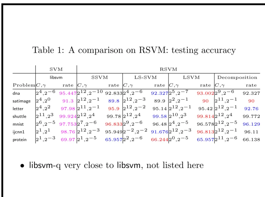
Table 1: A comparison on RSVM: testing accuracy

SVM RSVM

libsvm SSVM LS-SVM LSVM Decomposition

ProblemC,γ rate C,γ rate C,γ rate C,γ rate C,γ rate

dna 24,2−6 95.447212,2−10 92.83324,2−6 92.32725,2−7 93.00229,2−6 92.327 satimage 24,20 91.3 212,2−1 89.8 212,2−3 89.9 22,2−1 90 211,2−1 90 letter 24,22 97.98 211,2−1 95.9 212,2−2 95.14 212,2−1 95.42 212,2−1 92.76 shuttle 211,23 99.924212,24 99.78 212,24 99.58 210,23 99.814212,24 99.772 mnist 26,2−5 97.75327,2−6 96.83329,2−6 96.48 24,2−5 96.578212,2−5 96.129 ijcnn1 21,21 98.76 212,2−3 95.9492−2,2−2 91.676212,2−3 96.813212,2−1 96.11 protein 21,2−3 69.97 21,2−5 65.95722,2−6 66.24420,2−5 65.957211,2−6 66.138

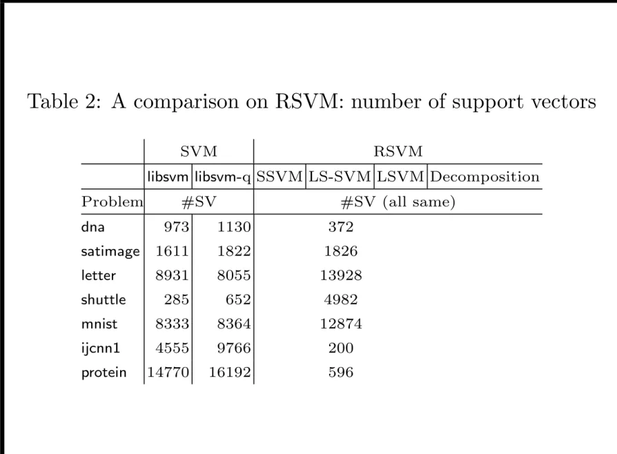
Table 2: A comparison on RSVM: number of support vectors

SVM RSVM

libsvm libsvm-q SSVM LS-SVM LSVM Decomposition Problem #SV #SV (all same)

dna 973 1130 372 satimage 1611 1822 1826 letter 8931 8055 13928 shuttle 285 652 4982 mnist 8333 8364 12874 ijcnn1 4555 9766 200 protein 14770 16192 596

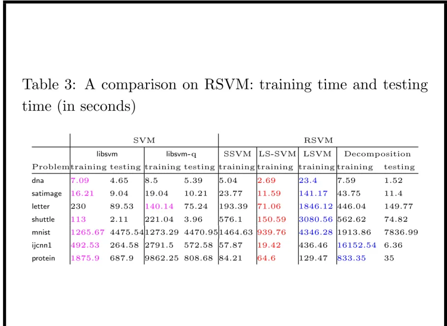
Table 3: A comparison on RSVM: training time and testing time (in seconds)

SVM RSVM

libsvm libsvm-q SSVM LS-SVM LSVM Decomposition Problemtraining testing training testing training training training training testing

dna 7.09 4.65 8.5 5.39 5.04 2.69 23.4 7.59 1.52 satimage 16.21 9.04 19.04 10.21 23.77 11.59 141.17 43.75 11.4 letter 230 89.53 140.14 75.24 193.39 71.06 1846.12 446.04 149.77 shuttle 113 2.11 221.04 3.96 576.1 150.59 3080.56 562.62 74.82 mnist 1265.67 4475.541273.29 4470.951464.63 939.76 4346.28 1913.86 7836.99 ijcnn1 492.53 264.58 2791.5 572.58 57.87 19.42 436.46 16152.54 6.36 protein 1875.9 687.9 9862.25 808.68 84.21 64.6 129.47 833.35 35

Observations

• Accuracy: all RSVM implementations lower than SVM • LS-SVM a little lower among RSVM implementations • Optimal models for RSVM have much larger C

• For median-sized problems RSVM not much faster • RSVM is much faster for ijcnn1 and protein

– larger problem or many support vectors for SVM – m is set small

• Find lower triangular V : V V T approximates a matrix • Primarily used for conjugate gradient methods

• Used for SVM in [Fine and Scheinberg, 2001]

– motivation: to solve SVM by interior point method, low-rank _{representation Q ∼ V V} T needed

– factorize Q

∗ large dense, entries calculated when needed ∗ only some ICF algorithms are suitable

ICF Algorithms

• Based on a columnwize Cholesky factorization method:  α v T v B   =   √ α 0 v √ α I    1 0 0 B − vv_αT     √ α √vT α 0 I   • 1st ICF algorithm in [Lin and Saigal, 2000]

– stores largest m values in each column of V – may fail: add βI and restart

• 2nd ICF algorithm in [Fine and Scheinberg, 2001]

– early stop, fewer columns of Cholesky factorization symmetric pivoting

• Linear SVM dual form: min α 1 2α T_{(Y X(Y X)}T _{+ yy}T )α − eTα 0 ≤ αi ≤ C, i = 1, . . . , l

• Approximate dual form by ICF, called ICFSVM: min α 1 2α T_{(V V} T _{+ yy}T )α − eTα 0 ≤ αi ≤ C, i = 1, . . . , l

Implementations

• Solving primal (SSVM,LS-SVM) versus

solving dual (LSVM, decomposition)

• ICFSVM in dual form: use decomposition to implement • Should we solve the corresponding primal?

min e w,ξ 1 2we T e w + C( l X i=1 ξi) subject to _{V ew ≥ e − ξ, ξ ≥ 0}

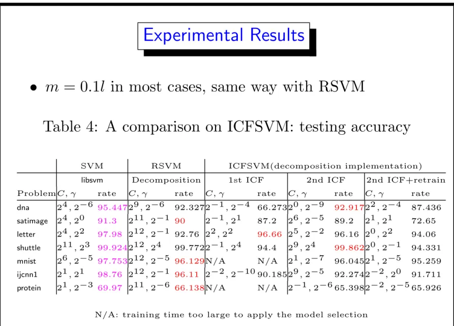
• m = 0.1l in most cases, same way with RSVM

Table 4: A comparison on ICFSVM: testing accuracy SVM RSVM ICFSVM(decomposition implementation) libsvm Decomposition 1st ICF 2nd ICF 2nd ICF+retrain ProblemC, γ rate C, γ rate C, γ rate C, γ rate C, γ rate dna 24, 2−6 95.44729, 2−6 92.3272−1, 2−4 66.27320, 2−9 92.91722, 2−4 87.436 satimage 24, 20 91.3 211, 2−1 90 2−1, 21 87.2 26, 2−5 89.2 21, 21 72.65 letter 24, 22 97.98 212, 2−1 92.76 22, 22 96.66 25, 2−2 96.16 20, 22 94.06 shuttle 211, 23 99.924212, 24 99.7722−1, 24 94.4 29, 24 99.86220, 2−1 94.331 mnist 26, 2−5 97.753212, 2−5 96.129N/A N/A 21, 2−7 96.04521, 2−5 95.259 ijcnn1 21, 21 98.76 212, 2−1 96.11 2−2, 2−10 90.18529, 2−5 92.2742−2, 20 91.711 protein 21, 2−3 69.97 211, 2−6 66.138N/A N/A 2−1, 2−6 65.3982−2, 2−5 65.926

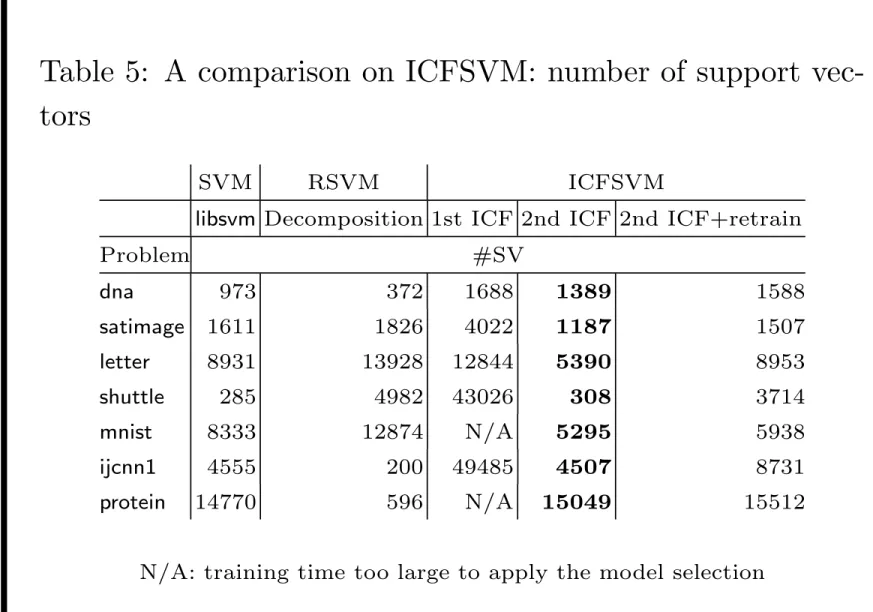
Table 5: A comparison on ICFSVM: number of support vec-tors

SVM RSVM ICFSVM

libsvm Decomposition 1st ICF 2nd ICF 2nd ICF+retrain

Problem #SV dna 973 372 1688 1389 ₁₅₈₈ satimage 1611 1826 4022 1187 ₁₅₀₇ letter 8931 13928 12844 5390 ₈₉₅₃ shuttle 285 4982 43026 308 ₃₇₁₄ mnist 8333 12874 N/A 5295 ₅₉₃₈ ijcnn1 4555 200 49485 4507 ₈₇₃₁ protein 14770 596 N/A 15049 ₁₅₅₁₂ N/A: training time too large to apply the model selection

time (in seconds)

SVM RSVM ICFSVM

libsvm Decomposition 1st ICF 2nd ICF 2nd ICF+retrain Problemtraining training training ICF training ICF training ICF

dna 7.09 7.59 440.41 427.18 9.62 5.45 33.77 5.52

satimage 16.21 43.75 558.23 467.48 48.49 28.37 61.59 28.32 letter 230 446.04 3565.31 2857.95 484.59 222.4 635.41 221.93 shuttle 113 562.62 70207.76 13948.141251.17 1184.631811.6 1265.51 mnist 1265.67 1913.86 N/A N/A 2585.13 2021.642565.08 1866.9 ijcnn1 492.53 16152.54 21059.3 4680.63 5463.8 103.97 1579.73 102.52 protein 1875.9 833.35 N/A N/A 217.53 92.52 3462.57 110.54

Discussions and Conclusions

• ICFSVM accuracy like RSVM, lower than SVM Used if decomposition for SVM cannot afford

• ICFSVM optimal models have smaller C than RSVM

• Support vectors of ICFSVM as sparse as SVM

• ICFSVM not faster than RSVM: ICF time too much

• Retrain SV from ICFSVM by SVM: not good • First algorithm strange: ICF may not close