具個別項目門檻值之效益挖掘

全文

(1)國立高雄大學資訊工程學系碩士論文 Department of Computer Science and Information Engineering National University of Kaohsiung Master Thesis. 具個別項目門檻值之效益挖掘 Utility Mining with Individual Item Thresholds. 研究生：趙育德 Student: Yu-Te Chao 指導教授：洪宗貝博士 Dr. Tzung-Pei Hong 藍國誠博士 Dr. Guo-Cheng Lan 中華民國 102 年 7 月 July 2013.

(2) 論文審定書. i.

(3) 致謝研究所的兩年求學歷程在這篇論文順利完成後寫下美麗的完結篇。回顧這兩年的時間裡，無非是在許多人的協助與鼓勵下，才能讓我順利完成碩士研究並且使此篇論文順利完成。首先，我要感謝的是我的指導教授，洪宗貝博士。老師在論文方向及研究的方法上總是給予許多寶貴的建議，在繁忙的教學研究過程中，老師還不時教導我們如何將研究的精華吸取為自己的知識，並不厭其煩的指導我們報告的要領。同時，也要深深地感謝學位考試的口試委員：黃健峯教授、李詠騏教授及林浚瑋教授。謝謝你們撥冗來參加，並給予寶貴的建議及指導，使我的論文更加完整。我也要感謝 AI 實驗室的的諸位學長姐、同學、以及學弟妹們。有你們在這些日子裡，不論是在平日與口試當天給予的幫助，都讓我這兩年研究生涯特別充實。特別是國誠學長，在我的研究過程不厭其煩地和我一起開會討論，並且以漸進式的討論方式讓我更快速的掌握重點，在我論文的修正投入了很大的心力協助，謝謝！最後也是最重要的，我必須深深地感謝我的家人們。有你們這兩年來對我的付出、鼓勵、包容及陪伴，使得我能夠專注在課業上。有你們的支持下，才能讓我在今天能夠順利地完成學業。. 趙育德. 2013.07.31. 謹誌於國立高雄大學. ii.

(4) 摘要. 近年來，效益挖掘因具有廣泛的實務應用，因此受到高度的重視，其主要原因為效益挖掘除了考慮在每筆交易記錄裡的購買項目資訊之外，亦考慮購買數量和項目利潤等其他因素，藉以評估每個項目在資料集裡之實際效益值，並以一個最小效益門檻值來決定資料集裡所有具有高效益之項目集。雖然此門檻值可用於鑑別各個項目是否為一個高效益項目，但是單一門檻檻並無法有效反映各個項目本身之重要性。因此，本論文介紹了一個具有各個項目之最小效益門檻值考量之研究議題，並命名為多準則效益挖掘。此外，當每個項目具有不同門檻值時，本論文也提出具有最小與最大結合條件之考量觀點，藉以決定一個具有多項目之項目集的適當門檻值。由於在最小結合條件觀點下，多準則效益挖掘即使在傳統效益上限模型裡仍是不具有向下封閉之特性，因此本論文設計一個具有排序策略的二階段挖掘方法來解決此問題。另一方面，在最大結合條件觀點裡，因在傳統效益上限模型裡可保持向下封閉之特性，所以，傳統二階段挖掘方法可很容易延伸來解決具有多個門檻值之多準則效益挖掘問題。最後，實驗結果顯示本論文所提出的兩種結合方法之有效性及在各種參數設定下之執行效率。. 關鍵字: 資料探勘，效益挖掘，最小約束，最大約束，多重門檻值. iii.

(5) Abstract Utility mining has recently attracted much attention due to its wide applications. It, however, considers the items uniformly by a single minimum utility criterion, such that the significance of the items is not actually reflected. How to develop an efficient and effective utility-based framework with the consideration of different item and itemset criteria is thus a critical issue. In this thesis, we introduce multi-criteria utility mining, which allows users to specify different minimum utility thresholds to items according to the characteristics or importance of items. In addition, two different viewpoints, respectively from minimum and from maximum constraints, are also presented to decide the utility threshold of an itemset when its items have different criteria. For the minimum constraint, the downward-closure property cannot be kept in the multi-criteria utility mining process. An effective sorting strategy and a two-phase multi-criteria approach are designed to cope with the problem.For the maximum constraint, the downward-closure property exists, such that the original two-phase approach can be easily extended to find high utility itemsets under multiple item thresholds. Finally, the experimental results on several simulation datasets show the effectiveness of the two viewpoints and the performance of the proposed approaches under different parameter settings. Keywords: Data mining, utility mining, minimum constraint, maximum constraint, multiple thresholds. iv.

(6) Content 論文審定書..................................................................................................................... i 致謝................................................................................................................................ii 摘要.............................................................................................................................. iii Abstract ......................................................................................................................... iv Content ........................................................................................................................... v List of Figures ..............................................................................................................vii List of Tables .............................................................................................................. viii CHAPTER 1 Introduction.............................................................................................. 1 1.1. Motivation ................................................................................................... 1. 1.2. Contributions............................................................................................... 4. 1.3. Organization of Thesis ................................................................................ 6. CHAPTER 2. Review of Related Works ..................................................................... 7. 2.1. Association-Rule Mining ............................................................................ 7. 2.2. Association-Rule Mining with Multiple Criteria ........................................ 8. 2.3. Utility mining ............................................................................................ 11. CHAPTER 3. Multi-criteria Utility Mining Using Minimum Constraints. ............... 14. 3.1. Introduction ............................................................................................... 14. 3.2. Problem Statement and Definitions .......................................................... 16. 3.3. The Proposed Algorithm(TPMmin) ............................................................ 22. 3.4. An Example of Using TPMmin Algorithm ................................................. 25. 3.5. Experimental Results ................................................................................ 34 3.5.1. Experimental Datasets ................................................................. 35. 3.5.2. Evaluation on Effectiveness of Minimum Constraints ................ 35. 3.5.3. Evaluation on Efficiency.............................................................. 37 v.

(7) CHAPTER 4. Multi-criteria Utility Mining with Maximum Constraints. ................ 40. 4.1. Introduction ............................................................................................... 40. 4.2. Problem Statement and Definitions .......................................................... 44. 4.3. The Proposed Approach(TPMmax) ............................................................. 49. 4.4. An Example of Using TPMmax Algorithm ................................................. 52. 4.5. Experimental Results ................................................................................ 60 4.5.1. Experimental Datasets ................................................................. 60. 4.5.2. Evaluation on Effectiveness of Maximum Constraints................ 61. 4.5.3. Evaluation on Efficiency.............................................................. 63. CHAPTER 5. Conclusions and Future Work............................................................. 66. References .................................................................................................................... 68. vi.

(8) List of Figures Figure 3.1: The numbers of HTWUs required by the approaches among various λmin.36 Figure 3.2: The numbers of HTWUs required by the approaches among various D. .. 37 Figure 3.3: Performance comparison of the two approaches under different λmin ....... 38 Figure 3.4: Performance comparison of the two approaches under different D .......... 38 Figure 4.1: The numbers of HTWUs required by the approaches under various λmin. . 62 Figure 4.2: The numbers of HTWUs required by the approaches under various D. .... 62 Figure 4.3: Performance comparison of the three approaches under different λmin. .... 64 Figure 4.4: Performance comparison of the three approaches under different D. ....... 64. vii.

(9) List of Tables Table 3.1: The ten transactions in this example ........................................................... 16 Table 3.2: The individual profit of items in the utility table ........................................ 17 Table 3.3: The individual threshold of items ............................................................... 17 Table 3.4: The set of ten transactions in this example ................................................. 25 Table 3.5: The profit of each item ................................................................................ 26 Table 3.6: The individual minimum utility threshold of each item ............................. 26 Table 3.7: The sorted transactions in this example ...................................................... 27 Table 3.8: The transaction utility values of the sorted ten transactions ....................... 28 Table 3.9: The transaction weighted utility ratios of all the items in this example ..... 29 Table 3.11: The results for the candidate 2-itmesets with the twur values .................. 31 Table 3.12: The set of HTWU2 ..................................................................................... 32 Table 3.13: The results for all the high transaction-weighted utilization itemsets ...... 32 Table 3.14: The results for all the high transaction-weighted utilization itemsets ...... 33 Table 3.15: The final set of high utility itemsets, HUs ................................................ 34 Table 3.16: Major parameters used in the experiments ............................................... 35 Table 4.1: The ten transactions in this example ........................................................... 44 Table 4.2: The individual profit of items in the utility table ........................................ 44 Table 4.3: The individual threshold of items ............................................................... 45 Table 4.4: The set of ten transactions in this example ................................................. 53 Table 4.5: The profit of each item ................................................................................ 53 Table 4.6: The individual minimum utility threshold of each item ............................. 53 Table 4.7: The transaction utility values of the sorted ten transactions ....................... 54 Table 4.8: The transaction weighted utility ratios of all the items in this example ..... 55 Table 4.9: The set of high transaction-weighted utilization 1-itemsets, HTWU1 ......... 56 viii.

(10) Table 4.10: The results for the candidate 2-itmesets with the twur values .................. 57 Table 4.11: The set of HTWU2 ..................................................................................... 57 Table 4.12: The results for all the high transaction-weighted utilization itemsets ...... 58 Table 4.13: The results for all itemsets with actual utility ratios in the set of HTWUs 59 Table 4.14: The final set of high utility itemsets, HUs ................................................ 59 Table 4.15: Major parameters used in the experiments. .............................................. 60. ix.

(11) CHAPTER 1 Introduction. 1.1 Motivation Data mining has received a lot of attention in knowledge discovery due to its wide applications. Among the various mining techniques, association-rule mining [3][4] was first proposed to find the co-occurrence relationship of items from a set of transactions. For example, assume that there is a product combination with high-frequency “{milk, bread}”, which means that most customers usually buy milk and bread together. To cope with this problem, Agrawal et al. presented a famous mining approach named Apriori to find association rules from databases [3][4]. The procedure of the Apriori approach [3][4] could be divided into the two phases: 1) Discovery of frequent itemsets; 2) Discovery of association rules. In the first phase, itemsets, whose actual supports were larger than or equal to a predefined threshold (called the minimum support threshold), were first found. Next in the second phase, association rules with high-confidence, which their confidence values satisfied the minimum confidence threshold, were induced from the set of previously found frequent itemsets. However, a transaction in a database usually includes other information, such as quantities and profits of items in that transaction other than item in1.

(12) formation. According to the principle of association-rule mining [3][4], the same importance is also assumed for all items in a database. It can be known that the association-rule mining techniques are not insufficient for recognizing the actual significance of an item in a database. To address this, Yao et al. then presented a new utility function, which considered both the profits and quantities of items bought in transactions to recognize actual utility values of itemsets [31], to discover high utility itemsets in a transaction database. Due to utility-based framework without downward-closure property, however, Liu et al. then proposed an effective upper-bound model [27], which is called the transaction-weighed utilization (abbreviated as TWU) model [27], to find all high utility itemsets in a database. The main concept of the TWU model is the summation of utility values of all items in a transaction as upper-bound of any subset in that transaction. Using the model [27], any information lose case in utility mining can be avoided, and then search space of finding high utility itemsets can be reduced to speed up execution efficiency in mining. However, although there exists only a single criterion (minimum utility threshold) for determining each item whether or not the item is a high utility item [31][27], a single criterion cannot be used to reflect the natures of the items, such as the significances of items. As mentioned in these studies [20] [26] [30], in real applications, 2.

(13) each item may have its own criteria to judge its importance. Then, the utility requirements should be varied along with different items. Accordingly, designing a framework with multiple minimum utilities to find all interesting high utility itemsets and how to find the interesting itemsets considering multiple minimum utilities are very critical issues. To our best knowledge, this is the first work on mining high utility itemsets with consideration of multiple minimum utilities in the field of utility mining. In the problem of multi-criteria utility mining, this thesis presents two approaches for finding interesting high utility itemsets with the consideration of minimum and maximum constraints. To find information desired by users, a minimum constraint based on multi-criteria utility mining is used to achieve this goal. Through the minimum constraint, lots of interesting utility itemsets whose utilities satisfy the minimum value of the criterions of all items in an itemset can be found. However, since the downward-closure property in utility mining cannot be directly applied to handle the problem of multi-criteria utility mining with minimum constraints, an effective model is designed to avoid any information lose case in mining. On the other hand, although minimum constraints can be used to find many interesting high utility itemsets in databases when items have different criteria, a large number of execution time is needed. To effectively speed up execution efficiency and 3.

(14) reduce number of interesting itemsets, another point of view is presented to define the minimum utilities of itemsets in the problem of multi-criteria utility mining. Based on the maximum constraint, the proposed second algorithm is easy and efficient when compared to the first approach using the minimum constraint. In addition, the number of high utility itemsets with the consideration of the maximum constraint is less than that using the minimum constraint. Whether to adopt the proposed first or second approach then depends on the requirements of mining problems. Based on the above reasons, this thesis presents a new research issue named multi-criteria utility mining (abbreviated as MUM), and also two kinds of viewpoints, minimum and maximum constraints, are presented to cope with the problems of multi-criteria utility mining. The motivation behind this thesis is to find lots of interesting utility itemsets with the consideration of multi-criteria utility, which may be provided more information for managers to make appropriate decisions in various practical applications.. 1.2 Contributions In this thesis, we propose two novel mining algorithms to achieve high performance for the new research issue named multi-criteria utility mining (abbreviated as MUM). In the general retail databases, transactions including items, quantities 4.

(15) bought and profits of the items are analyzed by the developed methods for multi-criteria utility mining (MUM). In the thesis, the major contributions of our studies are stated as follows: 1.. In this paper, we first propose a new research topic, namely multi-criteria utility mining, which considers that each item may have its own criteria to judge its importance in databases. In addition, we present two kinds of viewpoints, minimum constraint and maximum constraint, to define the proper criterion of an itemset in mining.. 2.. For multi-criteria utility mining with the minimum constraint, downward-closure property in utility mining cannot be kept in the problem. Thus, an effective strategy based on the traditional upper-bound model is developed to avoid any information lose case in mining, and a two-phase multi-criteria approach (TPMmin) using the effective strategy is presented to reduce search space of finding high utility itemsets with the consideration of minimum constraints.. 3.. In the problem of multi-criteria utility mining with the maximum constraint, downward-closure property in utility mining cannot be kept in the problem similarly. To solve this, the strategy based on the existing upper-bound model is designed to keep the property. In addition, a two-phase multi-criteria ap5.

(16) proach (TPMmax) using the effective strategy is proposed to find high utility itemsets when items have different minimum utilities. 4.. The experimental results show the proposed algorithms, TPMmin and TPMmax, have good performance in terms of effectiveness of itemsets and execution efficiency under various parameter settings when working with synthetic datasets generated by a public IBM data generator.. 1.3. Organization of Thesis. The rest of this thesis is organized as follows. We review the background and the related works including association-rule mining with with multiple minimum supports and utility mining in Chapter 2. The problem definitions for the proposed utility mining with minimum constraints and the experiments for the proposed TPMmin algorithm for finding high utility itemsets are described in Chapter 3. In addition, Chapter 4 then states the problem definitions for the proposed utility mining with maximum constraints and the experiments related to the proposed TPMmax approach. Finally, the conclusions and future of this work are given and discussed in Chapter 5.. 6.

(17) CHAPTER 2 Review of Related Works In this section, some related studies on association-rule mining, association-rule mining with multiple criteria and utility mining are briefly reviewed.. 2.1. Association-Rule Mining. Data mining techniques are used to extract useful information from various types of data. Among the published techniques, association-rule mining is one of important issues in the field of data mining due to the consideration of the co-occurrence relationship of items in transactions [3][4]. For example, assume there is a product combination with high-frequency, “{milks, breads}”, which presents that most customers usually buy the two products together in that supermarket. To find such information, Agrawal et al. proposed a well-known mining approach named Apriori to achieve this goal [3][4]. The process of Apriori algorithm could be divided into the two stages, (1) finding frequent itemset stage and (2) generating association rule stage. In the first stage, candidate itemsets were generated and then counted by scanning transaction data. If the count of an itemset in the transaction database was larger than or equal to the pre-defined threshold value (called minimum support threshold), the itemset was identified as a frequent one. Itemsets containing only one item were processed first. 7.

(18) Frequent itemsets containing only single items items were then combined to form candidate itemsets with two items. The above process was then repeated until no candidate itemsets were generated. In the second phase, association rules were derived from the set of frequent itemsets found in the first phase. All possible association combinations for each frequent itemset were formed, and those with calculated confidence larger than or equal to a pre-defined threshold (called the minimum confidence threshold) are output as the association rules. Afterward, many studies based on the framework of the Apriori approach had also been published to find association rules in databases [5][9][10][15][16].. 2.2. Association-Rule Mining with Multiple Criteria. As mentioned above, association rule mining only uses a single minimum support threshold to determine whether or not an item is frequent in a database [3][4]. However, in practical application, items may have different criteria to assess their importance [6][10][11][12][13][15][16][17][20][21][22][26][28][29][30]. That is, different items should be different support requirements. For example, the lower minimum support should be given the product “LCD TVs” with high-profit but low-frequency in a supermarket when compared with another product “Milks” with 8.

(19) low-profit but high-frequency. To address this problem, Liu et al. presented a new issue, namely association-rule mining with multiple minimum supports [26], which agreed the users to assign different minimum requirements for items by the significance of the items, such as profit or cost. However, since an itemset was composed of several distinct items, how to give the proper minimum support of the itemset is an important problem. To solve this, Liu et al. designed a minimum constraint to determine the minimum support of an itemset [26]. The main concept of the minimum constraint was that the minimum value of the minimum supports of all items in an itemset was regarded as the minimum support of that itemset. For example, assume there are three items, A, B and C, and the minimum supports of the three items are 0.3, 0.6 and 0.4, respectively. According to Liu et al.’s study [26], the minimum support of an assumed itemset {ABC} was 0.3 because the value of 0.3 was the minimum value of the three minimum supports for the three items, A, B and C. However, based on the minimum constraint, the minimum support of an itemset might be lower than the subset of the itemset. Continuing the above example, the minimum support of the itemset {ABC} is lower than that of its subset {B}. As this notes, the downwad-closure property in association-rule mining could not be kept in Liu et al.’s problem [26]. An effective strategy, which all distinct items in a database were sorted in ascending order of their 9.

(20) minimum support values, was proposed to achieve to solve this. Continuing with the above example, since the minimum supports of the three items A, B and C are 0.3, 0.6 and 0.4, a sorted list A, C and B can be obtained according to their minimum supports. With the help of the strategy, an Apriori-based approach in Liu et al.’s study [26] was developed to effectively find frequent itemsets when items had different minimum supports using the minimum constraint. Different from Liu et al.’s study [26], Wang et al. [30] presented a bin-oriented, non-uniform support constraint, which allowed the minimum support value of an itemset to be any function of the minimum support values of items contained in the itemset. The main concept is that items were first grouped into disjoint sets called bins, and items within the same bin were regarded as non-distinguishable with respect to the specification of a minimum support [30]. However, although their proposed approach is flexible in terms of assigning minimum supports to itemsets, performance of their mining approach is not good due to its generality [30]. To effectively reduce the time complexity, Lee et al. proposed another viewpoint, namely maximum constraint, to assign the minimum support requirement of an itemset [20]. Their proposed algorithm was easy and efficient under the maximum constraint when compared to the previous studies [26][30]. In Lee et al.’s study [20], the experimental results also showed the number of frequent itemsets using maximum 10.

(21) constraints was less than that using the minimum constraint, and thus the mined association rule set could be more compact.. 2.3. Utility mining. In real applications, a transaction in a transaction database usually involves quantities and profits of items other than the item information [3][4]. However, due to the consideration of only the occurrence relationship of items, association-rule mining is insufficient to be used to cope with such data [3][4]. For example, both jewel and diamond have high utility values but may not be frequent product combinations when compared to food and drink in a transaction database. Thus high-profit but low-frequency itemsets may not be found by the traditional association-rule mining approaches. To address this problem, Yao et al. proposed a utility function [31], which considered not only the quantities of the items but also their individual profits in transactions, to find high utility itemsets from a transaction database. According to Yao et al.’s definitions [31], local transaction utility (quantity) and external utility (profit) are used to measure the utility of an item. By using a transaction dataset and a utility table together, the discovered itemset is able to better match a user’s expectations than if found by considering only the transaction dataset itself. However, the downward-closure property in association-rule mining cannot be 11.

(22) directly applied in the utility mining problem [31]. To effectively reduce search space in mining, Liu et al. proposed a two-phase approach (abbreviated as TP) to efficiently handle the problem of utility mining [27]. In particular, an upper-bound model (called transaction-weighted utilization, TWU) was developed to keep the downward-closure property in mining [27]. The main principle of the model was that the summation of utility values of all the items in a transaction was regarded as the upper bound of any itemset in that transaction. The whole process of the mining algorithm could be divided into two phases. In the first phase, the promising itemsets with high utility upper-bounds were found from a transaction database by the TWU model [27]. Next in the second phase, an additional data scan was performed to find the actual utility of each promising itemset and found the ones that have actual utility values larger than or equal to a predefined threshold (called the minimum utility threshold). Afterward, most of existing approaches were based on the framework of the TP algorithm to copy with various applications with the viewpoint of utility mining, such as the efficiency improvement of utility mining [1][2][8][23][32], utility mining with negative item profits [7], on-shelf utility mining [18][19], incremental process for utility mining [24], and so on. As association-rule mining [3][4], one of main limitations for utility mining is that all the items are treated uniformly [27][31]. However, in real applications, differ12.

(23) ent items may have different criteria to judge their importance, and thus the utility requirements should vary with different items. Designing a utility-based framework with multiple minimum utilities is a critical issue. In addition, since the downward-closure property in association-rule mining is not kept in utility mining, the former is more difficult than the latter. Hence, how to develop an effective model for avoiding any information losing case is also another critical issue when items have different minimum utilities. As mentioned above, this motivates our exploration of the new issue, multi-criteria utility mining. In addition, two different viewpoints, minimum constraint and maximum constraint, are also considered in the multi-criteria utility mining problem, and two effective approaches are presented in the thesis to cope with the two problems.. 13.

(24) CHAPTER 3 Multi-criteria Utility Mining Minimum Constraints.. 3.1. Using. Introduction. Association-rule mining techniques consider only the co-occurrence frequency of items in transactions, but in retailing, transactions usually involve profits, costs and sold quantities of items. In addition, the same importance is assumed for all items in databases. Hence, the association-rule mining techniques are not insufficient to be used to recognize the actual significance of an item in databases. To address this problem, Yao et al. thus introduced a new utility-based framework [31], which considered both the quantities bought and profits of items in transactions to recognize the actual utility of itemsets in a database. With help of the utility function, itemsets with actual utilities larger than or equal to a predefined threshold (called the minimum utility threshold) could be found in databases [31]. However, all items in the utility-based framework are treated uniformly. That is, a single minimum utility is used as the utility requirement for all items in a database. As mentioned in these studies [6][10][11][12][13][15][16][17][20][21][22][26][28] [29][30], then, a single minimum utility is not easily used to reflect the natures of the 14.

(25) items, such as the significances of items. For example, in real world, since the profit of the item “LCD TV” is obviously higher than that of “Milk”, only a utility requirement is not easily used to reflect the importance of the two items. As this example notes, developing a utility-based framework with multiple minimum utilities is a critical issue. In addition, since the existing utility mining approaches cannot directly be applied to handle such utility mining problem. Accordingly, designing a proper mining method for avoiding any information losing case in the problem is also another critical issue. Due to the above reasons, this work presents a new research issue named multi-criteria utility mining, which allows users to define different minimum utilities for all items in databases. In particular, to find all possible interesting information, a minimum constraint is adopted in the work to achieve this goal. Based on the existing upper-bound model, an effective strategy, sorting, is designed to keep the downward-closure property in mining under the minimum constraint. In addition, a two-phase mining approach is also developed to cope with the problem of multi-criteria utility mining with the consideration of minimum constraints. The efficiency in finding high utility itemsets can thus be raised. Finally, the experimental results on synthetic datasets show the proposed approach has good performance in execution efficiency when compared with the state-of-the-art mining approach, TP. 15.

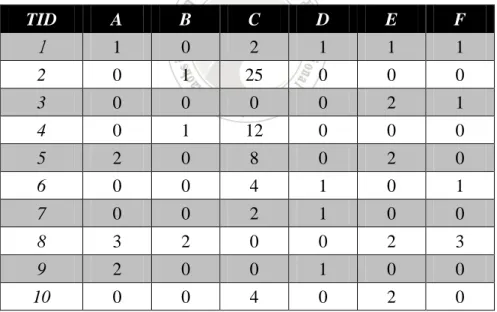
(26) The rest of this chapter is organized as follows. The problems to be solved and related definitions are described in Section 3.2. The execution details of the proposed two-phase mining TPMmin algorithm are introduced in Section 3.3. An example is presented in Section 3.4. Finally, the experimental results and discussions are then shown in Section 3.5.. 3.2. Problem Statement and Definitions. In this section, to clearly explain of the problem to be solved, a set of terms related to utility mining with multiple minimum utilities is then defined as follows. Table 3.1: The ten transactions in this example TID. A. B. C. D. E. F. 1. 1. 0. 2. 1. 1. 1. 2. 0. 1. 25. 0. 0. 0. 3. 0. 0. 0. 0. 2. 1. 4. 0. 1. 12. 0. 0. 0. 5. 2. 0. 8. 0. 2. 0. 6. 0. 0. 4. 1. 0. 1. 7. 0. 0. 2. 1. 0. 0. 8. 3. 2. 0. 0. 2. 3. 9. 2. 0. 0. 1. 0. 0. 10. 0. 0. 4. 0. 2. 0. 16.

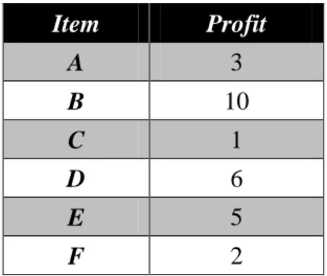
(27) Table 3.2: The individual profit of items in the utility table Item. Profit. A. 3. B. 10. C. 1. D. 6. E. 5. F. 2. Table 3.3: The individual threshold of items Item. Threshold. A. 0.20. B. 0.40. C. 0.25. D. 0.15. E. 0.20. F. 0.15. Definition 1. An itemset X is a subset of the items I, X ⊆ I. If | X | = r, the set X is called r-itemsets. I = {i1, i2, ..., in} is a set of items may appear in the transaction. For example, the 2-itemset {BC} includes two items, B and C. Definition 2. A transaction (Trans) consists of a set items purchased with their quantities. For example, in Table 3.1, the second transaction includes the two items, B and C, and the quantities of the two items are 1 and 25, respectively. Definition 3. A database D is composed of a set of transactions. That is, D = 17.

(28) {Trans1, Trans2, …, Transy, …, Transz}, where Transy is the y-th transaction in D. Definition 4. The quantity of an item i in a transaction Trnasy is called qyi. For example, in Table 3.1, the quantity of item A in a transaction Trnas1 is 1. Definition 5. The external utility si is the individual profit of an item i in the utility table. For example, in Table 3.2, the profit of item A in the utility table is 3. Definition 6. The utility uyi of an item i in Transy is the external utility si multiplied by the quantity qzj of i in Transy. That is,. u yi  si * q yi . For example, according to Table 3.1 and Table 3.2, the utility of item A in the first transaction can be calculated as 3*1, which is 3. Definition 7. The transaction utility tuy is the sum of the utility values of all items contained in Transy. That is, tui . . u. yi iTransy ^ Transy  D. ,. For example, the utility tu1 =3*1+1*2+6*1+5*1+2*1=18 in Table 3.1 and Table 3.2 Definition 8. The utility uyX of an itemset X in Transy is the summation of the utilities of all items in X in Transy. That is,. u yX . . u yi .. i X  X Transy. For example, according to the three tables, the utility of the itemet {AE} in the 18.

(29) first transaction can be calculated as 3*1 + 5*1, which is 8. Definition 9. The actual utility auX of an itemset X in a transaction database D is the summation of the utilities of X in the transactions including X of D. That is,. au X . . u. yX X Transy Transy D. .. For example, according to the three tables, the utility au{AE} of the itemset {AE} in Table 3.1 can be calculated as 8 + 16 + 19, which is 43. Definition 10. The actual utility ratio aurX of an itemset X in D is the summation of the utilities of X in the transactions including X of D over the summation of the transaction utilities of all transactions D. That is,. au X . . u. yX X Transy Transy D. .. For example, in Table 3.1, the summation of the transaction utilities of all transactions can be calculated as 18 + 35 + 12 + 22 + 24 + 12 + 8 + 45 + 12 + 14, which is 211. Since the actual utility au{AE} of the itemset {AE} in Table 3.1 is 48, the actual utility ratio au{AE} of {AE} in Table 3.1 can be calculated as 43/202, which is 0.2128. Definition 11. Let i be the predefined individual minimum utility threshold of an item i. Note that here a minimum constraint is used to select the minimum value of minimum utilities of all items in X as the minimum utility threshold X of X. Hence, an itemset X is called a high utility itemset (abbreviated as HU) if auX ≧X. For example, in Table 3.3, since the minimum utilities of the two items, A and E, 19.

(30) are all 0.2, the minimum value (= 0.2) is selected as the minimum utility threshold of {AE} is the value of 0.2. In Table 3.1, the actual utility ratio of the itemset {AE} is a high utility itemset under the minimum constraint due to its actual utility ratio (= 0.2128). Next to keep the downward-closure property in this problem the tradition-weighted utilization model (abbreviated as TWU) model is introduced to solve this problem. Then, a set of terms related to this model is described below. Definition 12. The transaction-weighted utility twuX of an itemset X in a transaction database D is the summation of the transaction utilities of the transactions including X in D. That is, twu X . . tu. y X Transy ^Transy QDB. ,. For example, in Table 3.3, since the itemset {AE} appears in the three transactions, Trans1, Trans5 and Trans8, and the transaction utilities of the three transactions are 19, 26 and 47, the transaction-weighted utility of {AE} can be calculated as 18 + 24 + 45, which is 87. Definition 13. The transaction-weighted utility ratio twurX of an itemset X in D is the summation of the transaction utilities of the transactions including X in D over the summation of transaction utilities of all transactions in D. That is,. 20.

(31) twurX . twu X ,  tu y. Transy D. For example, in Table 3.3, since the transaction-weighted utility of the itemset {AE} is 87, and the summation of all transactions in Table 3.1 is 211, the transaction-weighted utility ratio of {AE} can be calculated as 87/202, which is 0.4307. Definition 14. Let i be the predefined individual minimum utility threshold of an item i, and the minimum value of minimum utilities of all items in X is selected as the minimum utility threshold X of X by the minimum constraint. Hence, an itemset X is called a high transaction-weighted utilization itemset (abbreviated as HTWU) if twuX ≧X. For example, in Table 3.1, the itemset {AE} is a high transaction-weighted utilization itemset due to its transaction-weighted utility ratio (= 0.4307) and the minimum utility threshold (= 0.2).. Problem Statement: Based on the above definitions, the problem to be solved in this work is to find the itemsets with actual utilities larger than or equal to a pre-defined corresponding minimum utility threshold  from a given transaction database D under the minimum constraint. The details of the proposed TPMmin algorithm are then described in the next section.. 21.

(32) 3.3. The Proposed Algorithm(TPMmin). In this study, the proposed TPMmin algorithm based on minimum constraints consists of two phases, finding high transaction-utility upper-bound itemsets and finding high utility itemsets. The execution process of the TPMmin is then stated as follows.. INPUT: A set of items, each with a profit value and a minimum utility threshold, a transaction database D, in which each transaction includes a subset of items with quantities. OUTPUT: A final set of high utility itemsets (HUs) satisfying their minimum utilities.. Phase 1: Finding high transaction-weighted utilization itemsets (HTWUs) STEP 1: Sort the items in transactions in ascending order of their minimum utility values. STEP 2: For each transaction Transy in D, do the following substeps. (a) Find the utility uyz of each item iz in Transy. That is, u yz  v yz * si ,. (b) Find the transaction utility tuyz of Transy. That is,. tu y . . u .. yz iz Transy ^ Transy  D. 22.

(33) STEP 3: Find the total transaction utility of transaction utilities of all transactions in D. That is,. . ttu . tu y .. Transy  D. STEP 4: For each item i in D, calculate the transaction-weighted utility ratio twuri of item i as:. . twuri . tu. y iTransy ^ Transy  QDB. ttu. ,. STEP 5: Find the smallest value of the minimum utilities of all items in D, and denote as min,1. STEP 6: For each item i in D, if the transaction-weighted utility ratio twuri of i is larger than or equal to the corresponding minimum utility threshold i of the item i, put it in the set of high transaction-weighted utilization 1-itemsets, HTWU1. STEP 7: Set r = 1, where r represents the number of items in the current set of candidate utility r-itemsets (Cr) to be processed. STEP 8: Generate from the set HTWUr the candidate set Cr+1, in which all the r-sub-itemsets of each candidate must be contained in the set of HTWUr. STEP 9: For. each. candidate. (r+1)-itemset. X. in. the. set. Cr+1,. find. the. transaction-weighted utility ratio twurX of X in QDB as:. twurX . . tu. y X Transy ^Transy QDB. ttu. .. STEP 10: Find the first one of itemsets sorted in the set Cr+1 in ascending order of the. 23.

(34) minimum utility values of the itemsets, and find the smallest value of the minimum utilities of the items in the first itemset denote as min,r+1. STEP 11: For each candidate utility (r+1)-itemset X in set Cr+1, check whether the transaction-weighted utility ratio twurX of X is larger than or equal to the threshold min,r+1 under the minimum constraint. If it is, put it in set HTWUr+1. STEP 12: If HTWUr+1 is null, do STEP 9; otherwise, set r = r + 1 and repeat STEPs 7 to 10. Phase 2: Finding high utility itemsets (HUs) satisfying their minimum utilities STEP 13: Scan D once to the actual utility auX of X in all HTWU sets. That is, au x . . u. yX X Transy ^ Transy QDB. .. STEP 14: For each itemset X in all HTWU sets, do the following substeps. (a) Find the minimum value λi among all items in X as the minimum utility threshold λX of X under the minimum constraint. (b) Check whether the actual utility ratio aurX of X is larger than or equal to the minimum utility threshold λX. If it is, put it in set HUr+1. STEP 15: Output the final set of high utility itemsets satisfying their minimum utilities, HUs.. 24.

(35) 3.4. An Example of Using TPMmin Algorithm. In this section, an example is given to show how the proposed TPMmin algorithm can be easily used to find high utility itemsets in a transaction database. Assume there are ten transactions, each of which consists of three features, transaction identification (TID), items purchased, and quantities of the items in each transaction. Assume the transaction data is shown in Table 3.4 and are used for mining. Also, assume the profit and minimum utility threshold of each item are shown in Table 3.5 and Table 3.6, respectively. Table 3.4: The set of ten transactions in this example TID. A. B. C. D. E. F. 1. 1. 0. 2. 1. 1. 1. 2. 0. 1. 25. 0. 0. 0. 3. 0. 0. 0. 0. 2. 1. 4. 0. 1. 12. 0. 0. 0. 5. 2. 0. 8. 0. 2. 0. 6. 0. 0. 4. 1. 0. 1. 7. 0. 0. 2. 1. 0. 0. 8. 3. 2. 0. 0. 2. 3. 9. 2. 0. 0. 1. 0. 0. 10. 0. 0. 4. 0. 2. 0. 25.

(36) Table 3.5: The profit of each item Item. Profit. A. 3. B. 10. C. 1. D. 6. E. 5. F. 2. Table 3.6: The individual minimum utility threshold of each item Item. Threshold. A. 0.20. B. 0.40. C. 0.25. D. 0.15. E. 0.20. F. 0.15. To find all high utility itemsets in Table 3.4, the proposed mining algorithm proceeds as follows.. Phase 1: Finding high transaction-weighted utilization itemsets STEP 1: The items in each transaction are sorted in ascending order of their minimum utility values by Table 3.6. Take the first transaction as an example, it includes the five items, A, C, D, E and F, and the minimum utility values of the five items are 0.20, 0.25, 0.15, 0.20 and 0.15, respectively. The five items in Trans1 are sorted as D, 26.

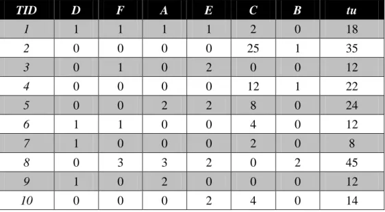
(37) F, A, E and C. The results for the sorted transactions are shown in Table 3.7.. Table 3.7: The sorted transactions in this example TID. D. F. A. E. C. B. 1. 1. 1. 1. 1. 2. 0. 2. 0. 0. 0. 0. 25. 1. 3. 0. 1. 0. 2. 0. 0. 4. 0. 0. 0. 0. 12. 1. 5. 0. 0. 2. 2. 8. 0. 6. 1. 1. 0. 0. 4. 0. 7. 1. 0. 0. 0. 2. 0. 8. 0. 3. 3. 2. 0. 2. 9. 1. 0. 2. 0. 0. 0. 10. 0. 0. 0. 2. 4. 0. STEP 2: The transaction utility of each transaction in Table 3.7 is found. Take the first transaction (Trans1) in Table 3.7 as an example, the transaction includes five items, A, C, D, E and F, and the quantities of the five items in Table 3.5 are 1, 2, 1, 1 and 1, respectively. In addition, the profits of the five items in Table 3.5 are 3, 1, 6, 5 and 2. Then, the utilities of the five items A, C, D, E and F in Trans1 are 3 (= 1*3), 2 (= 2*1), 6 (= 6*1), 5 (= 5*1) and 2 (= 2*1). In addition, the transaction utility of Trans1 can be calculated as 3 + 2 + 6 + 5 + 2, which 18. All the other transactions in Table 3.7 can be done for the same way. The transaction utility values of the transactions in Table 3.7 are shown in Table 3.8.. 27.

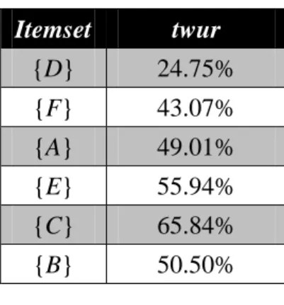
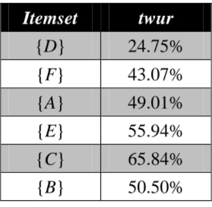
(38) Table 3.8: The transaction utility values of the sorted ten transactions TID. D. F. A. E. C. B. tu. 1. 1. 1. 1. 1. 2. 0. 18. 2. 0. 0. 0. 0. 25. 1. 35. 3. 0. 1. 0. 2. 0. 0. 12. 4. 0. 0. 0. 0. 12. 1. 22. 5. 0. 0. 2. 2. 8. 0. 24. 6. 1. 1. 0. 0. 4. 0. 12. 7. 1. 0. 0. 0. 2. 0. 8. 8. 0. 3. 3. 2. 0. 2. 45. 9. 1. 0. 2. 0. 0. 0. 12. 10. 0. 0. 0. 2. 4. 0. 14. STEP 3: The total transaction utility of all transactions in Table 3.8 are found. In this example, since the transaction utility values of the ten transactions are 18, 35, 12, 22, 24, 12, 8, 45, 12 and 14, respectively, the total transaction utility (ttu) can be calculated as 18 + 35 + 12 + 22 + 24 + 12 + 8 + 45 + 12 + 14, which is 202.. STEP 4: The transaction-weighted utility ratio (twur) of all items in Table 3.8 are found. Take item A in Table 3.8 as an example. It appears in the four transactions Trans1, Trans5, Trans8 and Trans9, and the transaction utility values of the four transactions are 18, 24, 45, 12, respectively. Then, the transaction-weighted utility ratio of {A} can be calculated as (18 + 24 + 45 + 12) / 202, which is about 49.01%. All the other items in Table 3.8 can be similarly processed. The results for the transaction-weighted utility ratio values of all the items in Table 3.8 are shown in Table 3.9. 28.

(39) Table 3.9: The transaction weighted utility ratios of all the items in this example Itemset. twur. {D}. 24.75%. {F}. 43.07%. {A}. 49.01%. {E}. 55.94%. {C}. 65.84%. {B}. 50.50%. STEP 5: In this example, since the possible items in Table 3.8 include the six items, A, B, C, D, E and F, and the minimum utilities of the six items in Table 3.6 are 0.2, 0.4, 0.25, 0.15, 0.2 and 0.15, respectively, the minimum value min among the six items are 0.15.. STEP 6: All high transaction-weighted utilization 1-itemsets can be found in Table 3.9. Take the 1-itemset {A} as an example. Since the transaction-weighted utility ratio twur{A} value of {A} is 49.01%, and the threshold min is 0.15, {A} is a high transaction-weighted utilization 1-itemset and is put in the set of high transaction-weighted utilization 1-itemsets, HTWU1. After this step, the results for all high transaction-weighted utilization 1-itemsets are shown in Table 3.10.. 29.

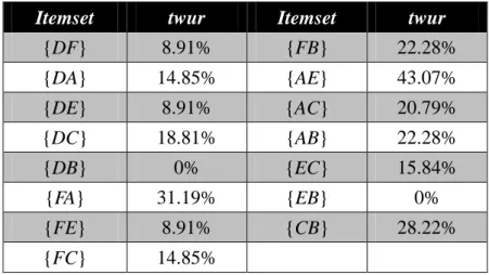
(40) Table 3.10: The set of high transaction-weighted utilization 1-itemsets, HTWU1 Itemset. twur. {D}. 24.75%. {F}. 43.07%. {A}. 49.01%. {E}. 55.94%. {C}. 65.84%. {B}. 50.50%. STEP 7: The variable r is currently set at 1, where r is used to represent the number of items in the candidate itemsets to be processed.. STEP 8: The candidate 2-itemsets are generated from the set of HTWU1. In this example, the fifteen 2-itemsets {DF}, {DA}, {DE}, {DC}, {DB}, {FA}, {FE}, {FC}, {FB}, {AE}, {AC}, {AB}, {EC}, {EB} and {CB} are put in the set of C2.. STEP 9: The transaction-weighted utility ratio values of the candidate 2-itemsets are found from Table 3.8. The process is the same as that mentioned previously in STEP 4. After this process, the results for the ten candidate 2-itemsets and their transaction-weighted utility ratio values are shown in Table 3.11.. 30.

(41) Table 3.11: The results for the candidate 2-itmesets with the twur values Itemset. twur. Itemset. twur. {DF}. 8.91%. {FB}. 22.28%. {DA}. 14.85%. {AE}. 43.07%. {DE}. 8.91%. {AC}. 20.79%. {DC}. 18.81%. {AB}. 22.28%. {DB}. 0%. {EC}. 15.84%. {FA}. 31.19%. {EB}. 0%. {FE}. 8.91%. {CB}. 28.22%. {FC}. 14.85%. STEP 10: In this example, the first itemset sorted in the set of C2 in ascending order of the minimum utility values of the itemsets is {DF}, and minimum utility values of the two items D and F in {DF} are all 0.15. Then, the minimum value among the two items D and F in {DF} is 0.15, and the value of 0.15 is used as the minimum utility threshold min,2 for finding high transaction-weighted utilization 2-itemsets, HTWU2.. STEP 11: The high transaction-weighted utilization 2-itemsets are found. Take the itemset {AE} as an example, the twur value of {AE} in Table 3.11 is 43.07%. In addition, the corresponding minimum utility threshold min,2 is 0.15. Then, {AE} is a high transaction-weighted utilization 2-itemset since its twur value is larger than or equal to the threshold min,2. Thus, the 2-itemset {AE} is put in the set of high transaction-weighted utilization 2-itemsets, HTWU2. All the other candidate 2-itemsets in Ta31.

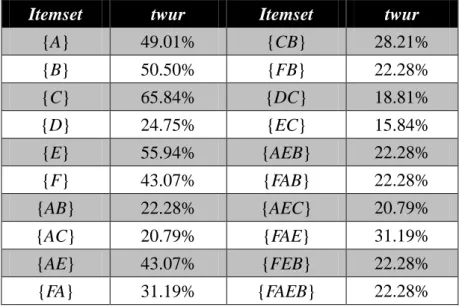
(42) ble 3.11 can be done in the same way. The results for all the high transction-weighted utilization 2-itemsets HTWU2 are shown in Table 3.12.. Table 3.12: The set of HTWU2 Itemset. twur. Itemset. twur. {EC}. 15.84%. {FB}. 22.28%. {DC}. 18.81%. {CB}. 28.22%. {AC}. 20.79%. {FA}. 31.19%. {AB}. 22.28%. {AE}. 43.07%. STEP 12: In this example, since set HTWU2 is not null, r is incremented to 2 and STEPs 8 to 12 are repeated. The whole mining task can be terminated until no candidate itemsets can be generated in the next pass. After the whole mining process, the twenty high transaction-weighted utilization itemsets are listed in Table 3.13.. Table 3.13: The results for all the high transaction-weighted utilization itemsets Itemset. twur. Itemset. twur. {A}. 49.01%. {CB}. 28.21%. {B}. 50.50%. {FB}. 22.28%. {C}. 65.84%. {DC}. 18.81%. {D}. 24.75%. {EC}. 15.84%. {E}. 55.94%. {AEB}. 22.28%. {F}. 43.07%. {FAB}. 22.28%. {AB}. 22.28%. {AEC}. 20.79%. {AC}. 20.79%. {FAE}. 31.19%. {AE}. 43.07%. {FEB}. 22.28%. {FA}. 31.19%. {FAEB}. 22.28%. 32.

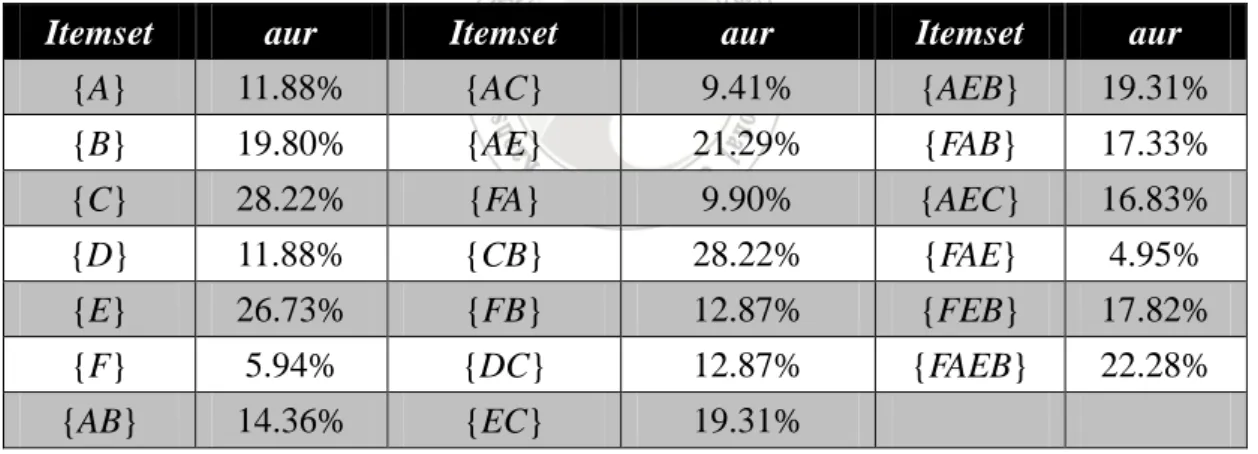
(43) Phase 2: Finding high utility itemsets satisfying their minimum utilities STEP 11: An additional data scan is executed for finding the actual utility value of each itemset in Table 3.13. Take the itemset {AE} in Table 3.13 as an example, it appears in Trans1, Trans5 and Trans8, and the utilities of {AE} in the three transactions are 8, 16 and 19. The actual utility ratio of {AE} can be calculated as (8 + 16 + 19) / 202, which is 21%. The other itemsets in Table 3.13 can be similarly processed. After this step, the results for all the itemsets and their actual utility ratios are shown in Table 3.14.. Table 3.14: The results for all the high transaction-weighted utilization itemsets Itemset. aur. Itemset. aur. Itemset. aur. {A}. 11.88%. {AC}. 9.41%. {AEB}. 19.31%. {B}. 19.80%. {AE}. 21.29%. {FAB}. 17.33%. {C}. 28.22%. {FA}. 9.90%. {AEC}. 16.83%. {D}. 11.88%. {CB}. 28.22%. {FAE}. 4.95%. {E}. 26.73%. {FB}. 12.87%. {FEB}. 17.82%. {F}. 5.94%. {DC}. 12.87%. {FAEB}. 22.28%. {AB}. 14.36%. {EC}. 19.31%. STEP 12: All the high utility itemsets can be found from Table 3.14. Take the itemset {BC} in Table 3.14 as an example. Since the minimum utility thresholds of B and C in Table 3.6 are 0.4 and 0.25, the minimum utility threshold of {BC} is the value of 0.25. Then, {BC} is a high utility itemset due to its actual utility ratio (= 28%) larger than or equal to its corresponding minimum utility threshold (= 0.25). The same process 33.

(44) can be done for the other itemsets in Table 3.14. The results for all high utility itemstes and their actual utility ratios are shown in Table 3.15.. Table 3.15: The final set of high utility itemsets, HUs Itemset. aur. Itemset. aur. {C}. 28.22%. { AEB }. 19.31%. {E}. 26.73%. { FAB }. 17.33%. {AE}. 21.29%. { AEC }. 16.83%. {CB}. 28.22%. { FEB }. 17.82%. {EC}. 19.31%. {FAEB}. 22.28%. {FE}. 17.33%. STEP 13: In this example, the eleven high fuzzy utility itemsets in the set of HUs, {C}, {E}, {AE}, {CB}, {EC}, {FE}, {AEB}, {FAB}, {AEC}, {FEB} and, {FAEB} are output as the decision makers’ auxiliary information.. 3.5. Experimental Results. A series of experiments were conducted to compare the performance of the proposed two-phase multi-criteria approach using minimum constraints (abbreviated as TPMmin) and traditional two-phase utility mining approach in Liu et al.’s study [27] in terms of the execution efficiency. The experiments were implemented in J2SDK 1.7.0 and executed on a PC with 3.3 GHz CPU and 8GB memory.. 34.

(45) 3.5.1. Experimental Datasets. In the experiments, the public IBM data generator [14] was used to produce the experimental data. The parameters used in the experiments are listed in Table 1. Table 3.16: Major parameters used in the experiments Parameter. Description. T. The average length of transactions. I. The average length of maximal potentially frequent itemsets. N. The total number of different items. D. The total number of transactions.  min. The set of minimum utility thresholds for items The minimum value of the minimum utility thresholds of all items. However, since our purpose was based on the problem of utility mining using the minimum constraints to discover high utility itemsets, we thus developed a simulation model, which was similar to that used in Liu et al.’s study [27], to generate the quantities of the items in the sequences. Each quantity ranged among 1 to 5 according to the described way in Liu et al.’s study [27]. Moreover, for each dataset generated, a corresponding utility table was also produced in which a profit value in the range from 0.01 to 10.00 was randomly assigned to an item.. 3.5.2. Evaluation on Effectiveness of Minimum Constraints. Experiments were first made on the synthetic datasets to evaluate the difference of. 35.

(46) high transction-weighted utilization itemsets (HTWUs) with and without the consideration of minimum constraints. Figure 3.2 and Figure 3.3 showed the difference on numbers of HTWUs with the two types of considerations under various min and D, respectively. Here the symbol min represented the minimum value of minimum utility thresholds of all items in databases, and min was regarded as the minimum utility. Number of High Transaction-Weighted Utilization Itemsets. threshold in traditional utility mining using only a single minimum utility, min_util. T10.I4.N4K.D200K Dataset 2,500 2,000 1,500. 1,000 500 0 0.20%. 0.40%. 0.60%. 0.80%. 1.00%.  min: Minimum Value of All Minimum Utilities TPMmin. TP. Number of High Transaction-Weighted Utilization Itemsets. Figure 3.1: The numbers of HTWUs required by the approaches among various λmin.. T10.I4.N4K.DxK Datasets, min = 0.20% 2,500 2,000 1,500. 1,000 500 0 100K. 200K. 300K. 400K. D: Number of Transactions TPMmin. 36. TP. 500K.

(47) Figure 3.2: The numbers of HTWUs required by the approaches among various D.. As shown in the figures, the number of high transaction-weighted utilization itemsets found by the proposed TPMmin was obviously less than that of TP using only the single minimum utility criterion, min_util under different min and D. The main reason for this is that all items in traditional utility mining were treated uniformly. That is, the traditional utility mining did not consider the individual importance of items, and thus the number of high transaction-weighted utilization itemsets was more than that with the consideration of different minimum utilities of items. According to the experimental results, we could know that it was necessary for considering the individual importance of items. Although the lower minimum utility threshold for traditional utility mining could be used to find more high transaction-weighted utilization itemsets, the number of found high transaction-weighted utilization itemsets was often huge. Hence, the proposed utility-based framework using minimum constraints might be a proper framework when items had different minimum utilities.. 3.5.3. Evaluation on Efficiency. Experiments were then made on the synthetic datasets to evaluate the execution efficiency of the proposed TPMmin approach and the traditional two-phase mining ap37.

(48) proach, TP. Figure 3.4 and Figure 3.5 showed the efficiency of the two compared approaches for the datasets under different parameter settings, min and D, respectively.. D10.I4.N4K.D200K Dataset. Execution Time (Sec.). 100 80. 60 40 20 0 0.20%. 0.40%. 0.60%. 0.80%. 1.00%.  min: Minimum Value of All Minimum Utilities TPMmin. TP. Figure 3.3: Performance comparison of the two approaches under different λmin. T10.I4.N4K.DxK Dataset, min = 0.2%. Execution Time (Sec.). 300 250. 200 150 100 50 0 100K. 200K. 300K. 400K. 500K. D: Number of Transactions TPMmin. TP. Figure 3.4: Performance comparison of the two approaches under different D. As could be seen in these figures, the proposed TPMmin approach was better than 38.

(49) the traditional TP approach in terms of execution efficiency when min decreased or D increased. The main reason is that with the help of the minimum constraints, only the itemsets, which satisfied their own minimum utility threshold and not the lowest minimum value of all minimum utilities for all items, could be generated in the databases. Accordingly, the proposed TPMmin approach did not need to generate a huge number of high utility itemsets than the traditional TP approach using only the single minimum utility threshold. Overall, the proposed TPMmin outperformed the traditional TP approach in execution efficiency under various parameter settings.. 39.

(50) CHAPTER 4 Multi-criteria Utility Mining with Maximum Constraints. 4.1. Introduction. Data mining technology is one of important phases in knowledge discovery due to its discovery capabilities [3][4][5][9][10][15][16]. In the data mining field, association-rule mining techniques considering the co-occurrence frequency of items in transactions have been widely used in various practical applications, such as mobile data, multimedia data, biomedical data, etc. However, in retailing, transactions usually involve profits, costs and sold quantities of items. In addition, the same importance is assumed for all items in databases. Hence, the association-rule mining techniques are not insufficient to be used to recognize the actual significance of an item in databases. Difference from traditional frequency-based framework, Yao et al. thus introduced a new utility function [31], which considered both the individual profits and quantities of items bought in transactions to find out actual utility values of itemsets, to discover high utility itemsets from a database. Finally, the itemsets, which had their actual utilities larger than or equal to a predefined threshold (called the minimum utility threshold), were then obtained from the database [31]. 40.

(51) However, the downward-closure property in association-rule mining cannot directly be applied to find high utility itemsets from a database. To solve this problem, Liu et al. then proposed an effective upper-bound model [27], which is called the transaction-weighed utilization (abbreviated as TWU) model [27], to find all high utility itemsets in a database. The main concept of the model is that the utility values of all the items in a transaction are summed up as the transaction utility and used as the upper bound of any subset in the transaction, and then the transaction-weighted utility of an itemset is then defined as the total transaction utility value of the transactions in which the itemset appears. With the help of the TWU model [27], Liu et al. also proposed a two-phase utility mining approach (named TP) to find high utility itemsets in a database. In the first phase, all promising itemsets with the transaction-weighted utilities larger than or equal to a user-defined minimum utility threshold can be found from a database. In the second phase, an extra database scan is executed to find actual utilities of the promising itemsets, and then all high utility itemsets with the actual utilities larger than or equal to a user-defined minimum utility threshold are found from the set of promising itemsets.. 41.

(52) As mentioned above, the same minimum utility in the utility-based framework is defined for all items in a database [1][2][8][23][32][7][18][19][24][27][31]. Such way still causes that many interesting utility patterns may not be found in databases. If the minimum utility value is lower, many unnecessary utility patterns are generated and outputted to users. In contrast, while the minimum utility value is higher, many interesting patterns may not be discovered. Furthermore, when different minimum utilities are assumed for items, for an itemset consisting of multiple distinct items, minimum utility value of the itemset is not easily to be determined because of individual minimum utilities of items. On the other hand, there exists still a big challenge in our proposed utility mining problem. That is, the downward-closure property in association-rule mining is still not kept in the proposed problem. However, the existing utility mining approaches cannot directly be applied to handle the utility mining problem with the consideration of individual minimum utilities of items. Accordingly, designing a proper mining method to find all desired patterns is also a critical issue. Due to the above reasons, a new research issue named multi-criteria utility mining, which individual minimum utilities are assumed for items, is thus introduced in this study. To effectively find all interesting utility itemsets, the minimum constraint is designed to select the minimum value among all items in an itemset as the minimum utility of that itemset. Based on the existing upper-bound model, a two-phase ap42.

(53) proach for handling multi-criteria utility problem using the maximum constraint (abbreviated as TPMmax). Moreover, an effective strategy is adopted to reduce the number of unpromising candidates in the mining process, thus avoiding unnecessary evaluation. The efficiency in finding high utility itemsets can thus be raised. Finally, the experimental results on synthetic and real datasets reveal the proposed approach has stable performance in execution efficiency, and can find more interesting utility pattern patterns when compared with the traditional utility mining with considering only one minimum utility. The rest of this chapter is organized as follows. The problem to be solved and its definitions are described in Section 4.2. The execution details of the proposed TPMmax algorithm are introduced in Section 4.3. An example is given to illustrate how to perform the mining process by using the proposed TPMmax algorithm in Section 4.4. The experimental results are then shown in Section 4.5.. 43.

(54) 4.2. Problem Statement and Definitions. In this section, to clearly explain of the problem to be solved, a set of terms related to utility mining with multiple minimum utilities using the maximum constraint is then defined as follows. Table 4.1: The ten transactions in this example TID. A. B. C. D. E. F. 1. 1. 0. 2. 1. 1. 1. 2. 0. 1. 25. 0. 0. 0. 3. 0. 0. 0. 0. 2. 1. 4. 0. 1. 12. 0. 0. 0. 5. 2. 0. 8. 0. 2. 0. 6. 0. 0. 4. 1. 0. 1. 7. 0. 0. 2. 1. 0. 0. 8. 3. 2. 0. 0. 2. 3. 9. 2. 0. 0. 1. 0. 0. 10. 0. 0. 4. 0. 2. 0. Table 4.2: The individual profit of items in the utility table Item. Profit. A. 3. B. 10. C. 1. D. 6. E. 5. F. 2. 44.

(55) Table 4.3: The individual threshold of items Item. Threshold. A. 0.20. B. 0.40. C. 0.25. D. 0.15. E. 0.20. F. 0.15. Definition 1. An itemset X is a subset of the items I, X ⊆ I. If | X | = r, the set X is called r-itemsets. I = {i1, i2, ..., in} is a set of items may appear in the transaction. For example, the 2-itemset {BC} includes two items, B and C. Definition 2. A transaction (Trans) consists of a set items purchased with their quantities. For example, in Table 3.1, the second transaction includes the two items, B and C, and the quantities of the two items are 1 and 25, respectively. Definition 3. A database D is composed of a set of transactions. That is, D = {Trans1, Trans2, …, Transy, …, Transz}, where Transy is the y-th transaction in D. Definition 4. The quantity of an item i in a transaction Trnasy is called qyi. For example, in Table 3.1, the quantity of item A in a transaction Trnas1 is 1. Definition 5. The external utility si is the individual profit of an item i in the utility table. For example, in Table 3.2, the profit of item A in the utility table is 3. Definition 6. The utility uyi of an item i in Transy is the external utility si multiplied by the quantity qzj of i in Transy. That is, 45.

(56) u yi  si * q yi . For example, according to Table 3.1 and Table 3.2, the utility of item A in the first transaction can be calculated as 3*1, which is 3. Definition 7. The transaction utility tuy is the sum of the utility values of all items contained in Transy. That is, tui . . u. yi iTransy ^ Transy  D. ,. For example, in Table 3.1 and Table 3.2, the utility of the first transactions can be calculated as 3*1+1*2+6*1+5*1+2*1, which is 18. Definition 8. The utility uyX of an itemset X in Transy is the summation of the utilities of all items in X in Transy. That is,. u yX . . u yi .. i X  X Transy. For example, according to the three tables, the utility of the itemet {AE} in the first transaction can be calculated as 3*1 + 5*1, which is 8. Definition 9. The actual utility auX of an itemset X in a transaction database D is the summation of the utilities of X in the transactions including X of D. That is,. au X . . u. yX X Transy Transy D. .. For example, according to the three tables, the utility au{AE} of the itemset {AE} in Table 3.1 can be calculated as 8 + 16 + 19, which is 43. Definition 10. The actual utility ratio aurX of an itemset X in D is the summation 46.

(57) of the utilities of X in the transactions including X of D over the summation of the transaction utilities of all transactions D. That is,. au X . . u. yX X Transy Transy D. .. For example, in Table 3.1, the summation of the transaction utilities of all transactions can be calculated as 18 + 35 + 12+ 22 + 24+ 12 + 8 + 45+ 12 + 14, which is 202. Since the actual utility au{AE} of the itemset {AE} in Table 3.1 is 43, the actual utility ratio au{AE} of {AE} in Table 3.1 can be calculated as 43/202, which is 0.2129. Definition 11. Let i be the predefined individual minimum utility threshold of an item i. Note that here a maximum constraint is used to select the maximum value of minimum utilities of all items in X as the minimum utility threshold X of X. Hence, an itemset X is called a high utility itemset (abbreviated as HU) if auX ≧X. For example, in Table 3.3, since the minimum utilities of the two items, A and E, are all 0.2, the minimum value (= 0.2) is selected as the minimum utility threshold of {AE} is the value of 0.2. In Table 3.1, the actual utility ratio of the itemset {AE} is a high utility itemset under the minimum constraint due to its actual utility ratio (= 0.2129). Next to keep the downward-closure property in this problem the tradition-weighted utilization model (abbreviated as TWU) model is introduced to solve this problem. Then, a set of terms related to this model is described below. 47.

(58) Definition 12. The transaction-weighted utility twuX of an itemset X in a transaction database D is the summation of the transaction utilities of the transactions including X in D. That is, twu X . . tu. y X Transy ^Transy QDB. ,. For example, in Table 3.3, since the itemset {AE} appears in the three transactions, Trans1, Trans5 and Trans8, and the transaction utilities of the three transactions are 18, 24 and 45, the transaction-weighted utility of {AE} can be calculated as 18+ 24+ 45, which is 87. Definition 13. The transaction-weighted utility ratio twurX of an itemset X in D is the summation of the transaction utilities of the transactions including X in D over the summation of transaction utilities of all transactions in D. That is, twurX . twu X ,  tu y. Transy D. For example, in Table 4.3, since the transaction-weighted utility of the itemset {AE} is 87, and the summation of all transactions in Table 4.1 is 202, the transaction-weighted utility ratio of {AE} can be calculated as 87/202, which is 0.4307. Definition 14. Let i be the predefined individual minimum utility threshold of an item i, and the maximum value of minimum utilities of all items in X is selected as the minimum utility threshold X of X by the maximum constraint. Hence, an itemset X is called a high transaction-weighted utilization itemset (abbreviated as HTWU) if twuX 48.

(59) ≧X. For example, in Table 4.1, the itemset {AE} is a high transaction-weighted utilization itemset due to its transaction-weighted utility ratio (= 0.4307) and the minimum utility threshold (= 0.2).. Problem Statement: Based on the above definitions, the problem to be solved in this work is to find the itemsets with actual utilities larger than or equal to a pre-defined corresponding minimum utility threshold  from a given transaction database D under the maximum constraint. The details of the proposed TPMmax algorithm are then described in the next section.. 4.3. The Proposed Approach(TPMmax). In this study, the proposed TPMmax algorithm based on maximum constraints consists of two phases, including the discovery of high transaction-weighted utilization itemsets and the discovery of high utility itemsets. The execution process of the TPMmax is then stated below. INPUT: A set of items, each with a profit value and a minimum utility threshold, a quantitative transaction database QDB, in which each transaction includes a subset of items with quantities. 49.

(60) OUTPUT: A final set of high utility itemsets (HUs) satisfying their individual minimum utilities.. Phase 1: Finding high transaction-weighted utilization itemsets (HTWUs) STEP 1: For each transaction Transy in QDB, find the utility uyz of each item iz in Transy. That is, u yz  v yz * si ,. where uyz and si represent the utility value of the item iz in Transy and the individual profit value of iz, respectively. STEP 2: For each item i in QDB, calculate the transaction-weighted utility twui of the item i as: twui . . tu. y iTransy ^Transy QDB. ,. where tuy is the transaction utility of the y-th transaction Transy in QDB. STEP 3: For each item i in QDB, if the transaction-weighted utility twui of the item i is larger than or equal to the corresponding minimum utility threshold. i. of the. item i, put it in the set of high transaction-weighted utilization 1-itemsets, HTWU1. STEP 4: Set r = 1, where r represents the number of items in the current set of can50.

(61) didate utility r-itemsets (Cr) to be processed. STEP 5: Generate from the set HTWUr the candidate set Cr+1, in which all the r-sub-itemsets of each candidate must be contained in the set of HTWU r. STEP 6: For each candidate (r+1)-itemset X in the set Cr+1, find the transaction-weighted utility twuX of X in QDB as: twu X . . tu. y X Transy ^Transy QDB. .. STEP 7: For each candidate utility (r+1)-itemset X in set Cr+1, do the following substeps. (a) Find the maximum utility λX among all items in X as the minimum utility threshold of X, λX. (b) Check whether the transaction-weighted utility twuX of X is larger than or equal to the minimum utility threshold λX. If it is, put it in set HTWUr+1. STEP 8: If HTWUr+1 is null, do STEP 9; otherwise, set r = r + 1 and repeat STEPs 5 to 8. Phase 2: Finding high utility itemsets (HUs) satisfying their minimum utilities STEP 9: Scan the database QDB once to the actual utility auX of X in all HTWU sets. That is, au x . . u. yX X Transy ^ Transy  QDB. ,. where uyX is the summation of the utilities of all items in X in Transy. 51.

(62) STEP 10: For each itemset X in all HTWU sets, do the following substeps. (a) Find the maximum utility λX among all items in X as the minimum utility threshold of X, λX. (b) Check whether the actual utility auX of X is larger than or equal to the minimum utility threshold λX. If it is, put it in set HUr+1. STEP 11: Output the final set of high utility itemsets satisfying their individual minimum utilities, HUs.. 4.4. An Example of Using TPMmax Algorithm. In this section, an example is given to show how the proposed TPMmax algorithm can be easily used to find high utility itemsets in a transaction database. Assume there are ten transactions, each of which consists of three features, transaction identification (TID), items purchased, and quantities of the items in each transaction. Assume the transaction data is shown in Table 4.4 and are used for mining. Also, assume the profit and minimum utility threshold of each item are shown in Table 4.5 and Table 4.6, respectively.. 52.

(63) Table 4.4: The set of ten transactions in this example TID. A. B. C. D. E. F. 1. 1. 0. 2. 1. 1. 1. 2. 0. 1. 25. 0. 0. 0. 3. 0. 0. 0. 0. 2. 1. 4. 0. 1. 12. 0. 0. 0. 5. 2. 0. 8. 0. 2. 0. 6. 0. 0. 4. 1. 0. 1. 7. 0. 0. 2. 1. 0. 0. 8. 3. 2. 0. 0. 2. 3. 9. 2. 0. 0. 1. 0. 0. 10. 0. 0. 4. 0. 2. 0. Table 4.5: The profit of each item Item. Profit. A. 3. B. 10. C. 1. D. 6. E. 5. F. 2. Table 4.6: The individual minimum utility threshold of each item Item. Threshold. A. 0.20. B. 0.40. C. 0.25. D. 0.15. E. 0.20. F. 0.15 53.

(64) To find all high utility itemsets in Table 4.4, the proposed mining algorithm proceeds as follows. Phase 1: Finding high transaction-weighted utilization itemsets STEP 1: The transaction utility of each transaction in Table 4.4 is found. Take the first transaction (Trans1) in Table 4.4 as an example, the transaction includes five items, A, C, D, E and F, and the quantities of the five items in Table 4.5 are 1, 2, 1, 1 and 1, respectively. In addition, the profits of the five items in Table 4.5 are 3, 1, 6, 5 and 2. Then, the utilities of the five items A, C, D, E and F in Trans1 are 3 (= 1*3), 2 (= 2*1), 6 (= 6*1), 5 (= 5*1) and 2 (= 2*1). In addition, the transaction utility of Trans1 can be calculated as 3 + 2 + 6 + 5 + 2, which 18. All the other transactions in Table 4.4 can be similarly processed. The transaction utilities of the transactions are shown in Table 4.7.. Table 4.7: The transaction utility values of the sorted ten transactions TID. A. B. C. D. E. F. tu. 1. 1. 0. 2. 1. 1. 1. 18. 2. 0. 1. 25. 0. 0. 0. 35. 3. 0. 0. 0. 0. 2. 1. 12. 4. 0. 1. 12. 0. 0. 0. 22. 5. 2. 0. 8. 0. 2. 0. 24. 6. 0. 0. 4. 1. 0. 1. 12. 7. 0. 0. 2. 1. 0. 0. 8. 8. 3. 2. 0. 0. 2. 3. 45. 9. 2. 0. 0. 1. 0. 0. 12. 10. 0. 0. 4. 0. 2. 0. 14. 54.