Solving job insertion problem in job shop scheduling using iterative improvement

(1)

Solving Job Insertion Problem in Job Shop Scheduling Using Iterative

Improvement

Te-Wei Chiang and Hai-Yen Hau

Department of Electrical Engineering

National Taiwan University

Taipei, Taiwan 10617

China

ABSTRACT

The goal of Yhis paper is to present a job-shop scheduling system based on iterative improvement to react to inconsis- tencies between a scheduling plan and the actual course of events on a shop floor. The iterative improvement approach starts with a complete but possibly infeasible schedule, then applies local search technique to improve the schedule. The system described in this paper creates incrementally a referencebredictive) schedule and maintains the schedule, reacting to both conflict and opportunity. In this paper, we focus on job insertion problems, which arise frequently in dynamic and stochastic world. Experimental results show the effi- ciency and effectiveness of this approach.

1. INTRODUCTION

The job shop scheduling problem can be defined as the allocation of machines over time to perform a collection of jobs while minimizing(maximizig) some performance criterion and satisfying the operation precedence constraints and resource constraints [4].

In real world applications, optimal schedules quickly break down due to the dynamic and stochastic nature of the factory environment. Unexpected events such as machine breakdown, operation tardiness, reworking, new orders, and so on, quickly force changes to previously planned activities. It is preferred to ppoduce schedules that are satisfactory and to maintain these schedules in the dynamic environment.

In the past, investigators divided the job shop control into two phases [7]. The fvst phase is to determine proper due dates for arriving jobs. The second phase is to control the work flow to meet the due dates. They applied variety of decision rules to set due-dates and then used some dispatch- ing rules to determine the sequence of the operations on each machine. The weakness of these approaches lies in the inability to provide acceptable due dates for the customer and to meet the due dates.

Based on the above observations, we are motivated to solve the two problems usually occurred in real world applications. The first problem is that customer may question how soon a new order can be delivered. At this time, the scheduler must be capable of evaluating the status of the shop floor and negotiating with the customer to make a good profit. The second problem is that the scheduler must be capable of maintaining the schedule to react to the dynamic

0-7803-3280-6/96/$5.00 '1996 IEEE

and stochastic world. For the first problem, since the deliv-

ery

date of each order can be precisely determined after the schedule being generated, we can generate a reference schedule and assign the delivery dates in the schedule as the due dates. For the second problem, we have to revise and maintain the schedule according to actual state of shop. Conse- quently, we propose an approach based on iterative improvement [lo], [ l l ] to solve these problems.

Chiang and Hau [l], [2] proposed an iterative improvement approach for railway scheduling problems. The iterative improvement approach starts with a complete but possibly infeasible schedule, then applies local search technique to improve the schedule. The iterative improvement approach has several inherent advantages, such as implemen- tation ease and the ability to both generate solutions and improve existing ones. The system described in this paper creates incrementally a referencebredictive) schedule and maintains the schedule, reacting to both conflict and opportunity, using the iterative improvement approach. In this paper, we focus on job insertion problems, which arise frequently in dynamic and stochastic world.

The remainder of this paper is organized as follows. In Section 2, we survey the job-shop scheduling problems and briefly introduce the local search and simulated annealing techniques. Section 3 gives the problem solving architecture for the dynamic rescheduling problems, especially for the job insertion problems, and describes the algorithms used in our approach. Then, for minimum makespan objective, a heuristic improvement approach that can improve the schedule quality is given in Section 4. Finally, Section 5 summarizes our approach.

2. OVERVIEW Job Shop Scheduling as Optimization

To describe the problem, the following notations are defined, where operation j of job i is referred to as operation

(i,j).

N : Number of jobs. M : Number of machines.

sij : Start time of operation (i,j).

cij : Completion time of operation (i,j).

ci : Completion time of job i, which is equivalent to the pij : Processing time of operation ( i , j ) .

mu : Machine selected to process operation ( i , j ) . d, : Due date of job i.

completion time of the last operation of job i.

(2)

T, : Tardiness of job i, which is defined as the amount of job completion time c, passes the job due date d,, i.e., m a { 0, c,

-

d,} .

The following assumptions are made for the problem: (1) all the jobs are available at time zero, (2) operation processing is assumed to be nonpreemptive, (3) processing time of the jobs on the machines are known beforehand.

Since our approach can easily adapt to different objective functions, the objective function J can be shop-time-based (e.g., minimum makespan) or due-date-based (e.g., minimum weighted tardiness). For the ease of illustration, we will consider to minimize makespan in this paper. That is

J I cy (1)

P

: minJ, (2)

c,,

IS,^+^

(i=l, 2,

...,

N;

j=1, 2,

...,

M-1) (3) A scheduling problem can now be formulated as follows: subject to precedence constraint:

capacity constraints:

if m, = m,>, , then sY

-

s , ~ , >p,.,, or s , ~ ,

-

s, >p,,

(i,i'=l, 2,

...,

N ; i#i'; j J = l , 2,

...,

M) ₍₄₎

(5)

s,I 2 0 (l=l, 2,

...) N>

(6)

processing time requirements: ready tame requirements:

Corresponding to the four types of constramts are four types (Type I

-

Type

Iv>

of conflicts that may arise during the scheduling process, each of which corresponds to one of the constraint type defmed above. Each conflict is associated with either one operation (Type I11 and Type

IV)

or two operations (Type I

-

Type 11).

cy,- s,, = p y (i=l, 2, ...,

N;

j = 1 , 2,

...,

M)

Fundamentals

Local Search: Local search [6] is one of the few success- 11 techniques for combinatonal optimization problems. Assume that vector x represents the set of values assigned to the decision variables and a neighborhood N(x) is defined for x . Now given a solution point xk and an objective function A x ) to be minimized (or maxunized), a solution point xk+l is searched from the neighborhood N(x3 of xt such that

Axtil)

< f l x J ( orAxk+,)

>Ax,)).

If such a point exists, then the similar process is repeated for xk+,. Otherwise, xk is retained as a local optimum with respect to N(x3. As such, a set of solutions is generated and each of them is locally improved within its neighborhood.

Simulated Annealing: Simulated annealing which has evolved from the statistical mechanics is another successful technique for solving combinatorial optimization problem

[8], [9]. Simulated annealing can be regarded as a variation of local search. The main difference is that, in simulated annealing, each solution point in the neighborhood of the current search point is selected with a certain probability for the next search step. Such a difference make it possible to keep the algorithm from getting stuck at a local optmum by permitting uphill moves.

3. JOB INSERTION

IN

JOB SHOP SCHEDULING Proposed Architecture

The scheduling problem is further complicated by unpre- dictable interruptions during the actual manufacturing process. A schedule is simply a forecast and changes will be forced by interruptions such as machine breakdown, operator absence, new orders, and so on, all of which quickly force changes to previously planned activities. In this paper, we focus on the rescheduling problem.

Problem Formulation: Mathematically, the problem can be formulated as a constrained optimization problem (see section 2). , We can transform the constrained optimization problem to unconstrained optimization problem via the incorporation of the constraint violations into the objective function.

Assume t h a t z i s a solution point (or a schedule). It can be expressed as

where N is the number of jobs and A4 is the number of machines. Each g4 is associated with operation ( i , j ) and corre- sponds to an start time, completion time, machine triplet [sg,

cg, 7nJ. The objective function is

where

Pm

represents the makespan (the time taken to complete all jobs) of the schedule, which is our measure for schedule quality; Qm is the cost due to the conflicts in schedule &and

A

is the Lagrange multiplier used to relax the constraint violations. We usually refer the objective function C@3 to the cost function of the problem. Q(J) can be defined as

Zk,

q k , where qk is an positive integer representing

the time interval the Mh conflict is violated, assuming there are K m conflicts in the schedule

X.

System Architecture: The four basic components in the proposed system are : Initial Scheduler, Repair Scheduler, Local Scheduler and Conflict Management. First, an initial schedule is established by the Initial Scheduler according to the predictive schedule and the affect of real environment. The Repair Scheduler then determines the repairing sequence of conflicts after Conflict Management finds all conflicts in the initial schedule. The sequence of conflicts to be repaired in the proposed system is based on the earliest-conflict-first heuristic that the earliest constraint violation will be solved fust. Since the earliest conflict will be solved fust, there exists a boundary on the time axis whose left side is conflict- free. Through the appropriate selection of the repair methods, the boundary will move to right gradually until the schedule is conflict-free. In local scheduling, the conflict given by Repair Scheduler is repaired in the direction of minimizing the objective function. As such, two schedulers, the Repair Scheduler and the Local Scheduler, cooperate in harmony to generate the complete schedule.

X = +

1 l i l N a n d l5jW (7)

cm

=

m

3

+ @@3 (8)

K M

Proposed Algorithm

In

a production system, it is important to handle unexpected orders after a production schedule has been developed. In this paper, we focus on this kind of rescheduling problems.

(3)

TABLE I DataForExarrqle 1.

Operation Job0 Job 1 Job2 Job3 Job4

Number M P M P M P M P M P

x7

0 o . , ?

i

.

i

; I

...

' 1 : 3 : 4 : ~ 0 0 8 0 9 0 8 0 9 0 8 1 1 8 1 4 1 8 1 4 1 8 2 4 9 2 9 4 9 2 9 4 9 3 3 5 3 6 3 5 3 6 3 5 4 2 2 4 3 2 2 4 3 2 2 M: MacheNWber P : ProceSsingTime ~~ 0 .

...

C...

...

c

...

,*

...

a

...

1

...

&&L;A.;

...

J

...

1 ...

...

r

...

r....

....

...,..

...,...

121-1

I

t

1 i

!

I o : :3 :

...

i

...

i...w..~...-:.--..:

-...-...;

...

l3I-l

!

i

1 : 3: 141.1

...

j

....

P i

.2

i

I

...

, .-Ja-;

...

4 ...

Fig. 1. The predictive schedule before insertion.

Job Insertion: In order to react to the real status of shop flow, we must revise the predictive schedule. We only need to modify the affected operation in the predictive schedule and feed the modified schedule into the system. Then the system will automatically repair the conflicts in the schedule and hence result in a new predictive schedule. But for new orders, the generation of iditial schedule is somewhat different. We have to put the new operations in appropriate posi- tion in the initial schedule, such that the resulting schedule is acceptable. Tbere are two approaches that can add a new job. First, insert each operation of the new job in a m m e r that the origiqal predictive schedule does not change. In other word, the schedule is still conflict-free aRer insertion. Second, the insertion of operations may result in capacity constraint violations, but it would increase the machine utilization and the resulting conflict-free schedule would be better. Now let's look at

an

example.

Example

I.

(Inserting New Orders) There is a ran- domly generated 5-job 5-machine problem. The data of the problem is given in Table

I.

Assume that there is a predictive schedule im which four jobs (Job-0 to Job-3) have been scheduled usiqg the SPT(shortest processing time) rule [4] (see Fig. 1).

In

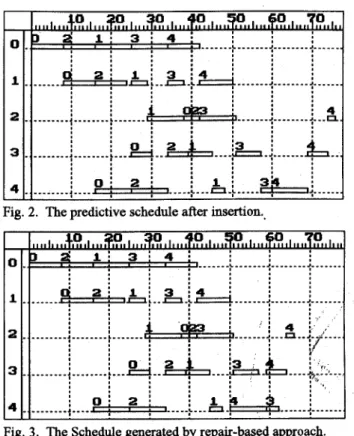
Fig. 1, each rectangle represents an operation and the number above the rectangle represents the job ID the operation belongs to. Then a new order, Job-4, comes. A straightforward approach to arrange Job-4, say pure inser- tion, is to insert each operation of the job to the earliest available time of the machine associated with the operation (see Fig. 2). Such approach makes the original schedule unchanged. The makespan of the resulting schedule is 76. It is poor compared to the one directly rescheduled by SPT

-

0 1 2 3 4

-

Fig. 2. The predictive schedule after insertion.,

Fig. 3. The Schedule generated by repair-based approach. rule, whose makespan is 66. Taking a close look at Fig. 2, we fuzd that the idle time between 50 and 57 on Machine-4 is redundant because the operation belonging to Job-4 can start earlier. But this possihility has been excluded by pure insertion because the machine idle time, 7, is not long enough to put the operation, whose processing time is 9. This motivates us to apply iterative improvement approach to solve the problem. Even though the machine idle time is not enough to insert

an

operation, we force the insertion of the operation such that the machine utilization is increased. Although conflicts may occur, they can be solved quickly by the iterative repair method described in the following subsec- tions. We expect that the makespan of the resulting schedule is shorter compared to pure insertion. In other word, the initial schedule is generated without considering whether the resulting schedule will change the original schedule or not. The resulting schedule is shown in Fig. 3, whose makespan is also 66.

Repair Methods: Recall that each conflict is associated with either one job (Type

111-IV)

or two jobs (Type

1-11).

When a conflict arises between two jobs on a machine, one of the jobs will be selected in an attempt to reduce the cost function as much as possible. The system will try to shift the operation left or right on the t m e axis so long as the resource is available, rather than exploring many possible alternatives. There are two repair methods that can repair a conflict: (1) Left-Shift(LS): left-shift the violated operation on the time axis such that the constraint is satisfied; (2) Right-ShiR(RS): right-shft the violated operation

on

the time axis such that the violated constraint is satisfied. To facilitate the selection of repair method for a conflict, we specify the priority of

(4)

Step 1. Generate the initial schedule; Find all conflicts in the initial schedule and put these conflicts to Sc; Evaluate c,

.

earliest conflict from SG Put all possible repair

methods to S,.

Step 3. Select and delete the highest priority repair method from SG Test to repair the selected conflict;

Evaluate c,,.

Step 4. If c,, < c, or S, is empty, then perform the repair and goto step 5, else goto step 3.

Step 5. Update Sc; c, := c,; Goto step 2.

Step 2. If S, is empty then stop, else select and delete the

Fig. 4. The iterative repair algorithm based on local search techniques.

each repair method, such that the repair method with higher priority will be tried fust. The priority of a LS is higher than that of a RS because moving operation right on time axis will cause the operation to occupy the resource longer and hence affect the performance of the schedule. Although RS has lower priority, it plays an important role in ow system. Since RS would not create conflict left of the conflict-free boundary on the time axis, if can facilitate the expansion of the conflict-free area.

Iterative Repair: During each iteration, we iteratively search a repair that resolves the conflict given by the

earliest-conflict-first heuristic while minimizing the cost

function. To select an appropriate repair method for a conflict, local search techniques can be used. If a repair reduces the cost function, then we accept the repair method, other- wise we try next priority repair method until all possible repairs to the conflict has been tried. If no repair method can reduce the cost function, the repair method with lowest priority, i.e., right shift, will be selected. This is somewhat different from the conventional local search which forbids all possible moves that increase the cost function. The local search algorithm is shown in Fig. 4, in which the following notations are used S, : the set of conflicts in the current schedule; S, : the set of repair methods; c, : the cost of the original schedule; c, : the cost of the new generated schedule.

4. HE,uRISTIC IMPROVEMENT Iterative Improvement Approach

Although the quality of the resulting schedule is good enough, one may question whether it can be further improved. In the past, a number of algoritbms based on iterative improvement approach have been developed to find a reasonably good schedule not necessarily the optimum one. Basically, an iterative improvement algorithm can be described as follows:

Iterative Improvement Algorithm

Step 1. Generate an initial schedule.

Step 2. Select a neighbor from the neighborhood of the current schedule.

/

2.1 Apply evaluation function.

2.2 Check admissibility.

Step 3 . Update the schedule status if a schedule is found, otherwise go back to step 2.

Step 4. Repeat steps 2 through 3 until done.

The neighborhood of a schedule can be defined as a set of schedules that can be obtained by applying the transition

function on the given schedule. A transition in the case of

job shop scheduling problem is generated by choosing vertices v and w, such that 191: (1) v and w are any two successive operations performed on the same machine k, (2) edge (v, w )

is a critical arc, i.e., (v, w) is on the critical path of the digraph; and reversing the order in which v and w are processed

on

the machine

k.

The transition function is based on the facts that it can never lead to an infeasible solution and the reversal of a noncritical arc cannot lead to a acyclic digraph with shorter critical path because the original critical path still exists.

Generally, a neighbor is randomly Lselected from the neighborhood 0fthe"current schedule. The admissibility of a neighbor is decided by the search techniques the iterative improvement algorithm used. The search techniques can be

local search [ 6 ] , simulated annealing [9], or tabu search [ 5 ] .

Disjunctive Graph Model

A disjunctive graph model (G) with a set of vertices ( V ) , a

set of arcs (A) and a set of edges (E) can be used for repre- senting the problem [9]. The set of vertices V consists of all the vertices and two vertices numbered 0 and P+1 representing the fictitious start and end operations respectively, assuming P is the total number of operations. The processing time of the operation is denoted as the weight of the vertex. The two fictitious operations 0 and P+1 have operation times of zero. The set A contains arcs connecting consecutive

operations of each job, as well as arcs from 0 to f i s t opera- tion of each job and from the last operation of each job to P+1. The edges in the set E connect operations to be proc-

essed by the same machine. The edges in the graph have two possible orientations. The assignment of orientations to these edges forms a schedule. It is easy to verify that any orientation of the edges which the resulting digraph is acyclic corresponds to a feasible sequencmg of the operations on the machines. Once the length of a path is defined as the sum of the weights of the vertices in the path, solving the job shop corresponds to finding an acyclic orientation of G such that the length of the longest path between 0 and P+1 is mini- mized. The longest path, called criticalpath, corresponds to the makespan (total time for completion of the operations of all the jobs) of the schedule. Thts is equivalent to finding the permutations of the operations on each machine to minimize the makespan. Taking the schedule shown in Fig. 3 for example, it can be represented as a disjunctive digraph as shown in Fig. 5 . In the figure, vertex 1 to 5 correspond to the five operations of Job-0, and vertex 6 to 10 correspond to the five operations of Job-1, and so on. The directed arcs between the vertices denote that the operations are to be

(5)

1 2 3 4 5

:

Fig. 5. The disjunctive graph associated with the schedule

h

Fig. 3. solid lines denote arcs in A and dashed lines denote edges in E.

processed in tbat order.

New Neighborhood Function

Contrast to traditional iterative improvement approach that randomly select a neighbor from the neighborhood, we propose a useful heuristic that can quickly find a good neighbor.

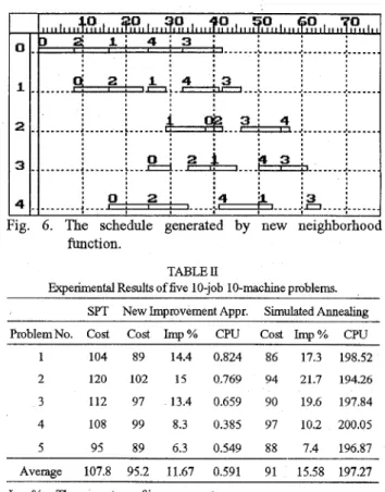
In Fig. 3, we can easily verify that the makespan is equivalent to the length of critical path. If we utilize the pair (Job-ID, %-ID) to identify a particular operation in the Gantt chart, then the critical path of the schedule is comprised of the following operations :(O,O), (2,0), (l,O), (3,0), (4,0), (4,1), (4,2), (4,3), (4,4). In other words, the summation of the processing times of these operations is equal to the makespan of the schedule. A straightforward idea to shorten the makespan is to move the last operation, (4,4), on the critical path earlier. Due to the precedence constraints, the only way i s to reverse the order of operation (3,O) a d operation (4,0), such that operation (4,4) can be performed earlier.

Based on the above observations, we develop a method of finding a good neighbor for the current schedule. The method is desaribed as follows:

Neighbor Finding Algorithm Step 1. Get i3 schedule.

Step 2. Find the critical path of the schedule. Step 3. Search the critical path backward.

3.1 Find the next operation pair (OPi, OPj) on the critical path, where OPi and OPj are performed on the same machme and OPi precedes OPj. 3.2 If no further operation pair can be found, then

output "no neighbor can be found" and stop. Step 4. If the relative priority factor RPF(OPi, OPj) is less

than zero, then reverse the order of the two operations, else goto back to step 3.

Step 5. According to the new operation sequences, gener- ate tbe resulting schedule.

From graph's point of view, the critical path is the longest

path between vertices 0 and P+1 and the length of the critical path is equal to the summation of the weights along the path; but from schedule's point of view, it corresponds to the summation of processing times of the operations along the path. A sequence of consecutive operations starting from the first operation of a job and ending at the latest operation of the schedule establish the critical path if the summation of the processing times of these operations is equal to the makespan. This is because the makespan is equal to the length of critical path. In step 5 of the neighbor finding algorithm, we have to generate a schedule from the given sequences. Given the operation sequences, there is only one schedule in which no superfluous idle time exists. The schedule can be obtained by semi-active timefabling [4].

The relative priority factor between OPi and OPj is de- fined as

RPF(OPi, OPj) = RM(0Pi) - RM(0Pj)

+

( m a { ctime[PJ[ OPj]

1,

ctime[PM[ OPi] ] }

-

stime( OPi)) where RM(0Pi) represents the remaining processing time of the job associated with the operation, which is equal to the summation of the processing times of the operations which subsequent to OPi and belong to the same job; RM(0Pj) is similar. Let PJ[OPi] denotes the immediate predecessor of operation OPi of the same job, and PM[OPi] denotes the immediate predecessor of operation OPi on the same machine; s h e [ . ] and ctime[.] denote the start time and the completion time of an operation respectively. The term, max{ctime[PJ[OPj]], ctime[PM[OPi]

I},

means the earliest start time of OPj after reversing the order of OPi and OPj. The underlying philosophy is that let the critical operations to start earlier in order to shorten the makespan. Moreover, after the reversion of the two operations on the critical path, the resulting schedule can be generated according the new sequence. The proposed heuristic improvement method can be described as follows:

Heuristic Improvement Algorithm Step 1. Get an initial schedule.

Step 2. Find the neighbor of the current schedule using the proposed neighbor finding algorithm.

2.1 If no neighbor can be found, then stop. 2.2 Set the neighbor as the current schedule.

2.2 If the current schedule is better than the best-so- far schedule, then set the schedule as the best-so- far schedule.

Step 3. Return to step 2.

Step 4. Repeat steps 2 through 3 until done.

It is worth noting that the proposed new neighbor does not guarantee that a better solution will be found after each step, but it largely increases the possibility of finding good solution after each step.

Example 2. Let us apply the new neighborhood function

to improve the schedule shown in Fig.3. The critical path of the schedule is comprised of the following operations

:(O,O),

(2,0), (1,0), (3,0), (4,O), (4,1), (421, (4,3), (4,4).

(6)

through the critical path backward, we can find the relative priority factor between (3,O) and (4,O) is -2. Since the two operations are perform on the same machine, Machine-0, and the relative priority factor between (3,O) and (4,O) is less than 0, it is worth while reversing the order of the two operations. The resulting schedule is shown in Fig. 6, whose makespan is 64. We can easily verify that the schedule is optimal. :3 : ....- ;o

_ _ _ _

L...

ip

5 ,

: 0 : 2 : 4 - - - . - - - {

_ _ _ _

J : I : I _ _ _ _ _ c Experimental Results

Numerical experiments were conducted using computer programs to evaluate the proposed method. In these experiments, we assume that each job has to be performed on each machine. The process time of each operation is uniformly distnbuted ~ f l interval [ 1 IO]. All experiments were run on a

PC 80486 DX-66. The computer program was written in C language.

Table I1 shows the computational results of five randomly generated 10-job 10-machine problems in terms of cost, the percentage of unprovement compared to SPT rule, and CPU tune. For the five problems, we find that the proposed unprovement approach can find better schedule with about 11.67 percent mprovement within 1 second. We also tested the same problems by simulated annealing techniques [8]. The mtial temperature, final temperature, decrement ratio, and the number of iterations at each temperature are set to 980, 1, 0.99, and 20 respectively. Although a near-optimal schedule can be found by simulated annealing techniques, the requred CPU tune is much longer.

5. CONCLUSIONS

In this paper, we demonstrated a job-shop scheduling system based on the iterative improvement for job insertion problems. We introduced how to transform the scheduling problem into an optimization problem. Through the coopera- tion of the earliest-conflict-first heuristic and local search techniques, the system can remove the conflicts in the reference schedule. Furthermore, we introduced a heuristic improvement method that can quickly improve the quality of the resulting schedule for minimum makespan objective. In conclusion, the proposed system can resolve the job insertion problems in an efficient and effective manner and can be applied to dynamic rescheduling problem s easily.

6. BFERENCES

[I] T. W. Chiang and H. Y. Hau, "Railway scheduling system using repair-based approach," in Proc. IEEE Int.

Con$ on Tools with Artijkial Intelligence, Washington

[2] T. W. Chiang and H. Y. Hau, "Cycle detection in repair- based railway scheduling system, " in Proc. IEEE Int.

Con$ on Robotics and Automation, Minnesota, vol. 3, pp. [3] M. Dell'Amico, M. Trubian, "Applying tabu search to the

DC, pp. 71-78, 1995.

2517-2522, 1996.

SPT New Improvement Appr. Simulated Annealing ProblemNo. Cost Cost Imp% CPU Cost Imp% CPU

1 104 89 14.4 0.824 86 17.3 198.52 2 120 102 15 0.769 94 21.7 194.26 3 112 97 13.4 0.659 90 19.6 197.84 4 108 99 8.3 0.385 97 10.2 200.05 5 95 89 6.3 0.549 88 7.4 196.87 Average 107.8 95.2 11.67 0.591 91 15.58 197.27 Imp % : The percentage of improvement

CPU : The CPU time being used

job-shop scheduling problem," Annals of Operations

Research, vol. 41, pp. 231-252, 1993.

[4] S. French, Sequencing and Scheduling: An Introduction

to the Mathematics of the Job-Shop. New York John

Wiley & Sons, 1982.

[5] F. Glover, "Tabu search - part I," ORSA J. Computing,

[6] J. Gu, "Local search for satisfiability (SAT) problem,"

IEEE Trans. on Systems, Man, and Cybernetics, vol. 23,

no. 4, pp.1108-1129, 1993.

[7] M. H. Han and L. F. Mcginnis, "Due dates in a manufacturing shop: an unweighted case," Annals of Oper. Res.,

vol. 17, pp.217-232, 1989.

[8] S. Kirkpatrick, C. D. Gelatt, and M. P. Vecchi, "Optimi- zation by simulated annealing," Science, vol. 220, no. [9] P. J. M. van Laarhoven, E. H. L. Aarts and J. K. Lenstra,

vol. 1, pp. 190-206, 1989.

4598, pp. 671-680,1983.

"Job shop scheduling by simulated annealing," Oper.

Res., vol. 40,no. 1, pp.113-125, 1992.

[lo] S. Minton, M. D. Johnston, A. B. Philips, and P. Laird, "Minimizing conflicts: a heuristic repair method for constraint satisfaction and scheduling problems,"

ArtiJicial Intelligence, vol. 58, pp. 161-205, 1992.

[ l l ] M. Zweben, E. Davis, B. Dam, and M. J. Deale, "Scheduling and rescheduling with iterative repair,"

IEEE Trans. on Systems, Man, and Cybernetics, vol. 23