Monitoring procedure for intelligent control: on-line identification of maximum closed-loop log modulus

(1)

Subscriber access provided by NATIONAL TAIWAN UNIV

Industrial & Engineering Chemistry Research is published by the American Chemical Society. 1155 Sixteenth Street N.W., Washington, DC 20036

Monitoring procedure for intelligent control: on-line

identification of maximum closed-loop log modulus

Ren Chiou Chiang, and Cheng Ching Yu

Ind. Eng. Chem. Res., 1993, 32 (1), 90-99 • DOI: 10.1021/ie00013a013

Downloaded from http://pubs.acs.org on November 28, 2008

More About This Article

The permalink http://dx.doi.org/10.1021/ie00013a013 provides access to: • Links to articles and content related to this article

(2)

90

better assess the design effort and the failure rate data required to develop safer designs.

Ind. Eng. Chem. Res. 1993, 32, 90-99

Grossmann, I. E.; Morari, M. Operability, Resiliency and Flexibility-Process Design Objectives for a Changing World. In the Proceedings of the Second International Conference on Acknowledgment

This work has been supported by NSF Grants DDM- 8616889 and CTS-9114050.

Literature Cited

Aelion, V.; Powers, G. J. A Unified Strategy for the Retrofit Syn- thesis of Flowsheet Structures for Attaining or Improving Oper- ating Procedures. Comput. Chem. Eng. 1991, 15 (5), 349-360. AIChE/CCPS. Guidelines for Hazard Evaluation Procedures;

Center for Chemical Process Safety, AIChE: New York, 1985. AIChE/CCPS. Guidelines for Chemical Process Quantitative Risk Analysis; Center for Chemical Process Safety, AIChE: New York, NY, 1989a.

AIChE/CCPS. Guidelines for Chemical Process Equipment Relia- bility Data; Center for Chemical Process Safety, AIChE: New York, NY, 1989b.

Crooks, C. A.; Macchietto, S. A Combined MILP and Logic-Based Approach to the Synthesis of Operating Procedures for Batch Plants. T o be published in Chem. Eng. Commun. 1992. Delboy, W. J.; Dubnansky, R. F.; Lapp, S. A. Sensitivity of Process

Risk to Human Error in an Ammonia Plant. Plantloper. Prog. Department of Labor, Occupational Safety and Health Administra- tion. Process Safety Management of Highly Hazardous Chemi- cals; Notice of Proposed Rulemaking. Fed. Reg. 1990, July 17, 29150-29173.

Englund, S. M.; Mallory, J. L.; Grinwis, D. J. Prevent Backflow. Chem. Eng. Prog. 1992,88 (2), 47-53.

Fusillo, R. H.; Powers, G. J. A Synthesis Method for Chemical Plant Operating Procedures. Comput. Chem. Eng. 1987, 1 I , 369-382. Fusillo, R. H.; Powers, G. J. Computer-Aided Planning of Purge

Operations. AIChE J. 1988a, 34, 558-566.

Fusillo, R. H.; Powers, G. J. Operating Procedure Synthesis using Local Models and Distributed Goals. Comput. Chem. Eng. 198813, 1991, 10 (4), 207-211.

12, 1023-1034.

Foundations

07

Co’rnputer-Aided Design, Snowmass’, CO, June 19-24; CACHE Publications; Ann Arbor, MI, 1983.

Huang, Y. L.; Fan, L. T. A Distributed Strategy for Integration of Process Design and Control: An Artificial Intelligence Approach for Incorporation of Controllability into Process Design. Pres- ented at the Annual AIChE Meeting, San Francisco, CA, Novem- ber, 1989; paper 27e.

Lakshmanan, R.; Stephanopoulos, G. Synthesis of Operating Pro- cedures for Complete Chemical Plants. Part I: Comput. Chem. Eng. 1988a, 12, 985-1002.

Lakshmanan, R.; Stephanopoulos, G. Synthesis of Operating Pro- cedures for Complete Chemical Plants. Part 11: A Nonlinear Planning Methodology. Comput. Chem. Eng. 1988b, 12, Lakshmanan, R.; Stephanopoulos, G. Synthesis of Operating Pro- cedures for Complete Chemical Plants. Part 111: Planning in the Presence of Qualitative Mixing Constraints. Comput. Chem. Eng. Lapp, S. A.; Powers, G. J. Computer-Aided Synthesis of Fault-Trees.

IEEE Trans. Reliab. 1977, 2, 13.

Powers, G. J.; Lapp, S. A. A Short Course on Risk and Reliability Assessment by Fault Tree Analysis. Manuscript in preparation, 1989.

Pistikopoulos, E. N.; Grossmann, I. E. Optimal Retrofit Design for Improving Process Flexibility in Linear Systems. Comput. Chem. Eng. 1988, 12 (7), 719-731.

Shaeiwitz, J. A.; Lapp, S. A.; Powers, G. J. Fault Tree Analysis of Sequential Systems. Ind. Eng. Chem. Process Des. Dev. 1977,16 The Bureau of National Affairs. The Clean Air Act Amendments: BNA’s Comprehensive Analysis of the New Law; Washington, DC, 1991.

Umeda, T. Computer Aided Process Synthesis. in PSE’82 Pro- ceedings; Kyoto, Japan, August 23-27; 1982; pp 79-109.

Received f o r review May 22, 1992 Revised manuscript received August 18, 1992 Accepted October 6, 1992 1003-1021.

1990,14, 301-317.

(41, 529-549.

Monitoring Procedure for Intelligent Control: On-Line Identification of

Maximum Closed-Loop Log Modulus

Ren-Chiou Chiang and Cheng-Ching

Yu*

Department of Chemical Engineering, National Taiwan Institute of Technology, Taipei, Taiwan 10672, R.O.C.

A

monitoring procedure is proposed to decide whether a retuning of the controller is necessary. The well-known robustness measure, maximum closed-loop log modulus

(LC,,=),

is used t o indicate the appropriateness of the controller parameters. T h e monitoring procedure identifies the maximum closed-loop log modulus in two t o three relay feedback experiments, a frequency domain approach. This procedure is tested against linear and nonlinear systems as well as systems with and without noise. The results show that the proposed method is very accurate in finding L,,,,, in an efficient manner.

1. Introduction vances in the theoretical aspects (Sastrv and Bodson, 1989. Chemical processes are nonlinear in nature, and they are

often operated at different operating conditions. There- fore, an ideal process control system should be able to maintain good performance at different operating points. Several methods can be employed to handle plant/model mismatches as the results of nonlinearity and/or changing operating conditions. One approach is the adaptive control where the process model and the controller are updated as the operation condition changes. Despite recent ad-

Chapter 3), adaptive control does not fit well into the process control environment, the operator-dominated operation. This is typically true when the more complex scenario of start-up, shutdown, override, alarm, etc. is considered. Another approach is the robust control (Morari and Zafiriou, 1989, Chapter 2) where a controller is designed for a range of operation conditions. However, when a large range of operation conditions is considered, achievable performance can be quite limited. This is the tradeoff that has to be made between the ranae of operation conditions considered and achievable performance. In our view, an ideal process control system should have

*

To whom correspondence should be addressed.

(3)

Ind. Eng. Chem. Res., Vol. 32, No. 1, 1993 91 robust performance in a smaller range of operation points.

Once the process drifta out of

this

range, on-line redesigned is made.

Therefore, an ideal control system should be able to monitor the robustness (or performance) of a close+loop system., The concept of expert control system of Arz6n (19891, Astrom et al. (1986), Doraiswami and Jiang (1989), and Ortega et al. (1992) offers some light in achieving this goal. The performance measure in expert control system generally is based on the errors in the controlled variable (e.g., integrated absolute error or integrated square error), a time domain technique. However, for the regulatory oriented process control systems, this means we are not able

to

access the robustness (or performance) of a control system until a disturbance comes into the system.

A

better measure should be able

to tell

the robustness of a closed- loop system before the disturbance comes into the system

(or significant deviations in the controlled variable are observed).

Recent advances in

H,

control theory (Zames, 1981; Francis, 1987) lead

to

a better approach for the design of a robust control system. The

H,

norm (llHll,) provides a good measure of robustness. For single-input-single- output

(SISO)

systems, the

H ,

norm is exactly the largest magnitude of the complementary sensitivity function, HGu)

= GGuFGw)/(l

+

GuuFGu,),

over the entire frequency range

(w = 0-). In the classical control theory, this is the maximum closed-loop log modulus (LC,,,; Luyben, 1990, p 484) or the M-circle (Ogata, 1970, p 441). For a fixed parameter controller, the

L,,,

often changes with operation conditions. A large L,,, indicates that the control system can tolerate a small amount of uncertainties. Therefore, it provides a good measure of robustness. Conventionally, L,,, is evaluated off-line. Typically, a process model is identified first, and the resonant peak of the closed-loop Bode plot is found. For on-line applications, this approach is time-consuming. The purpose of

this

work is to find a method for the on-line indentification

The success of &&om and Hiigglund (1984) autotuner leads to renewed interest in the relay feedback systems (Luyben, 1987; Astrom and Hlgglund, 1988; Chiang et al., 1992). The relay feedback system has the following advantages: (1) it is a closed-loop test and (2) it is quite efficient (requires much less time). These two advantages are quite useful for slow varying chemical processes. Furthermore, relays with hysteresis give frequency responses a t different frequencies (Ogata, 1970, p 546; Shih, 1982, p 270; Astrom and Hiigglund, 1988, p 44). Therefore, in this work, the relay with hysteresis is employed to find the L,,,. Since a relay feedback experiment only gives the response a t one frequency, an efficient method (within two to three experiments) is necessary for on-line applications. This paper is organized as follows. Section 2 relates the hysteresis of a relay to the

L,,,.

An on-line search method is proposed to find the L,, in section 3. Section 4 discusses the selection of hysteresis width followed by applications in section 5. The conclusion is presented in section 6.

2. Relay with Hysteresis and

Lp,ms.

2.1. Relay

Feedback

Systems. Astrom and Hiigglund (1984) proposes the use of a relay feedback system as a simple means to identify critical process information, the ultimate gain

K,,

and the ultimate frequency w,. Based on

this

process information, a crude estimate of the process model is readily available for controller tuning, e.g., the Ziegler-Nichols method or tuning methods based on the gain or phase margin (Astrom and Hagglund, 1988,

of

Lc,rn.**

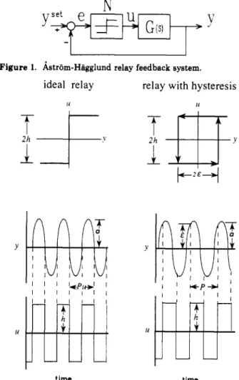
Figure 1. Astrom-Hiigglund relay feedback system.

ideal relay

Y

k

I 1

I I

time

relay with hysteresis I 1 Y

w

I I

I

vi

y:

I I n p r time

Figure 2. Relay feedback experiments for ideal relay and relay with hysteresis.

Chapter 4; Luyben, 1990, p 482; Seborg et al., 1989, p 298). In the Astrom-Hagglund relay feedback system (1984), an ideal relay is inserted between the process output and control output (u) (Figure 1). In a relay feedback ex- periment, the relay responds to process output y (yset = 0) as shown in Figure 2. The sustained oscillation generated from the relay feedback leads to the critical in- formation about G(s): the ultimate gain

(K,)

and the ultimate frequency (w,),

K, = 4h/xa (1)

w, = 27r/P, (2)

where h is the height of the relay set by the user, a is the amplitude of the process oscillation, and

P,

is the ultimate

period. One important feature of the (ideal) relay feedback system is that it identifies the point when the Nyquist curve of Guu) crosaes the negative real axis GGw)~upcc,,,=-lao..

This can be analyzed from the describing function analysis (Ogata, 1970, p 546; Shih, 1982, p 270). Consider the feedback system in Figure 1, where N denotes the describing function of an ideal relay. The characteristic equation is

(3)

If eq 3 is satisfied, i.e.

1

+

G

,

?

= 0

(4) then the system exhibits a limit cycle. For an ideal relay, we have

(4)

92 Ind. Eng. Chem. Res., Vol. 32, No. 1, 1993

Im

I

rl-

I I

_ _ _ _ _ _

_ _ _ _ _ _ _ _ _ _ _ _

- _ _ - -

1 _ _ - _ _ _ _ _ _ _ _ _ _

I

Figure 3. Nyquist curve of Cow, and -1/N loci.

Graphically, this can be understood by plotting the -1/N loci on the Gu,,-plane (Figure 3). For an ideal relay, the

- 1 / N corresponds to the negative real axis and the in- tersection of -1/N loci and the Nyquist curve of G,,, is characterized by the limit cycle. This frequency can be found from the period of oscillation w, = 2r/PU, and the magnitude IG,,

,I

can be obtained from eq 5. All this information can 'be found directly from the relay feedback experiment.

2.2, Relay with Hysteresis. It is advantageous to have a relay with hysteresis inserted in the feedback loop (Figure

l), since the frequency responses of Gu,, a t phase angles other than -180° can be obtained. Figure 2 shows a relay with hysteresis, and t is the width of the hysteresis. Again,

the feedback system exhibits sustained oscillations and the corresponding point in the Nyquist curve is

where o is the specific frequency where the oscillation occurs (can be found from Figure 2 , w = 2a/P), h is the relay height, a is the amplitude of the process output, and

e is the hysteresis width (Figure 2 ) . The describing function analysis (-l/N loci) shows that the introduction of relay with hysteresis (ei in Figure 3) simply helps us to find the frequency responses of G w ) with phase angles

greater

than

-1800 (between -900 an8 -1800 to

be

specific).

It then becomes obvious that we are able to find the frequency responses of Gu,, at the third quadrant by changing

t. In other words, instead of going through the frequency

domain

to

find

Gu,,

(in the third quadrant), one can find G ), by changing t.

%or a specific frequency with a given relay height h and a given hysteresis width eo, we have

For a fixed h, the output amplitude a. is a function of G

as well as t. In a general form, we have

a = fcc,, (7)

Therefore, the frequency responses of G quadrant with a given h can be expresseyas

in the third

Note that the numerical value of Cow! is a function of t.

Since the function G appears implicitly in the RHS

Figure 4. Relay feedback monitoring system: m standing for monitoring mode and c standing for control mode.

(right-hand side) of eq 8, a further simplification is necessary for on-line applications (section 3). Nonetheless, eq 8 forms the basis for the monitoring procedure.

2.3. A Framework for Monitoring. Unlike the ap- plication of relay feedback systems in autotuning (Figure

l), performance monitoring is to detect situations where a complete retuning of the controller is necessary. Therefore, the monitoring is different from the autotuning in that a controller is known beforehand.

For the purpose of monitoring, a relay (N) is placed between the controller ( K ) and the process (G; Figure 4). Figure 4 shows that, in the monitoring mode, the input to the relay is the controller output ii and the output from the relay u goes directly into the process. In the control mode (c in Figure 4), the controller output goes into the process directly. Figure 4 reveals that this framework differs substantially from autotuning in spirit. However, in analysis, the technique involved is exactly the same as that of the autotuning system.

Again, the describing function analpis shows that, when the relay feedback system exhibits sustained oscillations, we have

According to eq 8, again, we have

(9)

Since we are monitoring the robustness of the closed-ioop system, the complementary sensitivity function Hti,, plays an important role.

(10)

Substituting eq 9 into eq 10, we have

In theory, the maximum closed-loop log modulus (Lcm,) can be found by searching for the resonant peak in lHuw)l

over the entire frequency range.

L,,,, 20 log (max

lH~,)l)

w

However, eq 11 reveals that, instead of searching over the frequency domain, we are able to find

L,,,,

by going through the t-domain. Let

(5)

-

Linear assumption

00000 Step by step

=r

E l

-

_E

Figure 5. Linear assumption for the relationship between a and c

in a relay feedback system with hysteresis.

From eq 13, a simple way to find

L,,,

is going through all possible e’s to find the largest

F,,).

However, in an operating environment, it is nearly impossible to monitor the system performance by going through endless relay feedback experiments (Figure 4). An efficient method is necessary if the monitoring procedure is of any practicality. 3. On-Line Search for

L,,,,,

3.1. Linear Assumption. The difficulty associated with eq 13 is that the amplitude of the oscillation a is a function of e as well as GK.

a = f G K ( t )

If

an approximation of f C K can be found by taking the effect of GK into account, eq 13 can be solved explicitly Graphically, the amplitude of the oscillation a can be viewed

as

the distance between the origin and a corresponding point in the Nyquist curve (scaled by ~ / 4 h ) and an increase in e correaponds to moving down the imaginary axis (Figure 3). A typical Nyquist curve of GKv,) in the third quadrant shows a monotonic increasing relationship between a and c, e.g., Figure 3. The simplest approximation for the amplitude of oscillation is

a = f C K ( f ) = me

+

a. (14)

where

m

is the slope which is characterized by GK, e is the hysteresis width, and a. is the amplitude of the oscillation when an ideal relay is applied (Figure 5). This approximation (eq 14) turns out to be an extremely accurate estimate of f C K (see examples in section 5). A typical example is shown in Figure 5, where the linear assumption (eq 14) approximates quite well the true amplitude. The open circles (step-by-step) denote the amplitude (a’s) obtained from exhausted relay feedback experiments. Also, in Figure 5, the slope m is found from two relay feedback experiments (e = 0 and e = el).

From eq 14, it becomes obvious that the Nyquist curve of GK is characterized by the slope m and the intersection

a@ For a given intersection ao, once the slope m is chosen, the Nyquist curve is fixed (at least in the third quadrant)

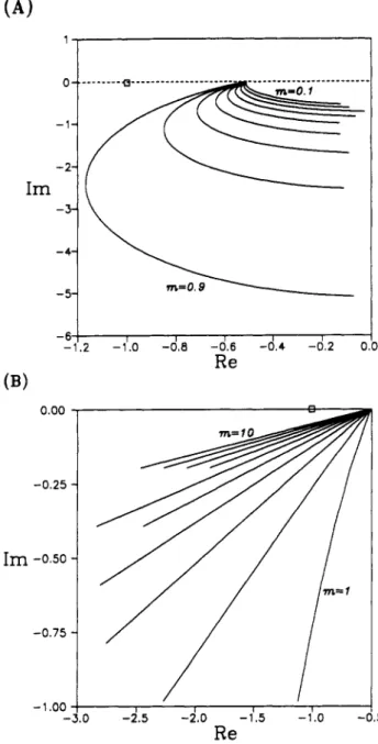
as shown in Figure 6. These curves (Figure 6) generally are capable of describing typical Nyquist curve of GK for open-loop stable G with a PI type of controller. For system with small values of m, the phase angle of GK is very sensitive to the changes in e. Since normally we do not have a priori knowledge about the shape of the Nyquist for Lc,m=*

Ind.

Eng.

Chem. Res., vol. 32, No. 1, 1993 93

-6

‘

1 I I -11.2 -1I.O -d.8 -0.6 -0.4 -0.2 0

R e

(B)

0.00 -0.25

Im

-0.50 -0.75

-

1 .oo m

/

I

I I I I ) -2.5 -2.0 -1.5 -1.0

-

R e

Figure 6. Nyquist curves of GK,, for different values of m (eq 14) for a given ao: (A) 0 < rn < 1 and (B) m 2 1.

curve, a small value of e is generally recommended to avoid spurious solutions.

Since the linear assumption (eq 14) is made

to

characterize the Nyquist curve of Gv,).Kl~), justification

to

such an assumption should be provide Obviously, the linear assumption is the simplest poasible form to correlate a and e. However, this assumption characterizes the inherent

shape of the Nyquist curve of GK. It is difficult to describe the appropriateness of this assumption according to the classification of G(,,, e.g., first-order systems, second-order systems, or systems with time delay, since the controller parameters change the shape of the Nyquist curve. The following theorem states the global property of the Nyquist curve characterized by the linear assumption.

Theorem. The Nyquist curve of Gv,Fv,) generated from a relay feedback system (eq 9) provided with the linear assumption (a = me

+

ao) shows the clockwise property.

PROOF.

See the Appendix for the proof.

Most control engineers have undoubtly noted that the Nyquist curves of stable systems tend to be clockwise (Horowitz and Ben-Adam, 1989; Tesi et al., 1992). In other

(6)

94 Ind. Eng. Chem. Res., Vol. 32, No. 1, 1993

words, most reasonably designed systems give clockwise Nyquist curves. Certainly, the assumption made (eq 14)

will have difficulty in characterizing the Nyquist curve with counterclockwise behavior [can be conjectured as non- monotonicity in the phase and magnitude of

GGwFGw)

(Tesi et al., 1992)] near resonant frequency.

It should be emphasized here that the approximation made here does not guarantee the closed-loop log modulus

L, is very accurate over the entire frequency range. For example, the success of the autotuning procedure of Astrom and Hagglund is because it identifies the critical process information

(K,

and w,) accurately. Similarly, this approach gives a good estimate of L, at an important frequency range (where L,, is most likely to occur) if the inherent limitation (clockwise property) is not violated.

32. Formulation. Once the linear assumption is made, the formula for the computation of L,,, can be con- structed. Substituting eq 14 into eqs 1 2 and 13, L,,,

becomes

Lc,max = 20 lodm- F(c)l

+

(

4h

)]-1'21

(15)

a(me

+

ao)

The maximum of F(6) can be found analytically by solving

C 4 t 4

+

c3t3

+

c2t2

+

c,c

+

co = 0 (16) where co = 0 2 - Ea02 c , = 2BD - BmEa, ~2 = B2

+

2AD - E(m2 - 1) ~3 = 2AB c4 = A2 and A = m 3 - m B = 2m2ao

+

a. D = mao2 E = ( 4 h r n / ~ ) ~

Therefore, the hysteresis width 7 corresponding to

L,,,,

can be calculated from eq 16. Notice that 7 is a positive value. Substituting 7 into eq 15, L , , is readily available.

3.3. Procedure. From the on-going analysis, it becomes clear that two relay feedback experiments are needed to find L,,,. An ideal relay (Figure 4) feedback is used to find the intersection a. (Figure 5 ) followed by a relay feedback with hysteresis (c) to find the slope m (eq 14). Once a. and m are available, L , ,

can

be calculated from eqs 15 and 16.

Therefore, the monitoring procedure

can

be summarized as follows.

1. Switch the control system to the monitoring mode (m in Figure 4).

2. Perform an ideal relay feedback experiment and record the amplitude ao.

3. Perform another relay feedback experiment with a hysteresis e (t

>

0) and record the amplitude a,.

4. Calculate the slope rn (of eq 14) from ao, a,, and t (rn

= (al

-

ao)/t).

5. Calculate 7 from eq 16.

6. Calculate

L,,,,

from eq 15.

Steps 1-6 complete the monitoring procedure. If necessary, one can perform an additional relay feedback experiment using the hysteresis width 7 to validate the result

(to check the difference between the approximated and the true L,,,,).

3.4. Limitations. The proposed monitoring procedure generally can find L,,,, in an efficient manner. Several limitations of the proposed method should be noticed. Since a negative value of the hysteresis height t is not

physically realizable, the on-line search for L,,, is con- fined to the third quadrant. Therefore, if the L,,, is

located outside the third quadrant, e.g., the second quadrant, the method fails. Certainly, this problem can be overcome by inserting an artificial element, e.g., a deriv- ative term "s", such that the search space for the phase angle falls between -180' and -270' (the third quadrant) instead of -90' and -180' (the second quadrant).

Another problem associated with the proposed method is the linear assumption (eq 14). The linear assumption basically assumes that the Nyquist curve of GKciw, has the clockwise property. In a less rigorous argument, the magnitude and phase of

Gvw)Ktiw)

are monotonically de- creasing functions with respect to w. This assumption generally holds when the controller has integral action. However, if the vicinity of the resonant frequency (of HGw)) exhibits nonmonotonic behavior in GKGw), the linear assumption can give poor result (despite the fact that it rarely happens, since the nonmonotonic behavior in GKOw,

generally happens (if it exists) a t the frequency smaller than the resonant frequency).

4. Selection of Hysteresis Width

4.1. Noise-Free Systems. Technically the choice of the relay width t also plays an important role for the

successful finding of Lc,,,. Figure 6 shows that, for systems with small value of m, the phase angle of G K,,,

decreases rapidly to -90' for a small increase in t. d%!hout

a priori knowledge about the shape of GG,,Kti,), a small value o f t is preferred to ensure the successful character- ization of GGwFtiw,. Therefore, for a noise-free system, the principle is to select t as small as possible.

4.2. Systems with Noise. Any practical monitoring procedure should be able to handle process noise. In process control systems, the noises come from measuring devices, control valves, or the process itself. In relay feedback experiments, the amplitude of the limit cycle is often corrupted with noises. In that case, the relay height should be adjusted such that a good (large) signal-to-noise ratio is ensured.

In selecting hysteresis width, a small E is preferred for

noise-free systems. However, too small a c can lead to the switching of relay as the result of process noises. Consider a sequence of normally distributed noise w ( t ) with zero mean inserted between the controller K and the relay N (Figure 4). Since the amplitudes of the limit cycles are corrupted with noise, the selection of t should be recon-

sidered. In the monitoring procedure the slope (m in eq 14) are calculated from

where the subscript N denotes the condition under noise. In other words,

(18) with w i ( t )

E

[-a,a]. A simple principle is to assure that

(7)

Ind. Eng. Chem. Res., Vol. 32, No. 1, 1993 95 -0.5

'

0.4 1 -0.2

4

-0.4

1

0.4 0.2

u

0.0 -0.2 -0.4 0.32

Lineo r ossum pt ion Step by step 0.30 0.24 0.00 0.03 0.06 0.09 0.12 0. E -0.6

'

, I

6

160 260 $0 460 560 600

Figure 7. Relay feedback experiments for example 1.

m N is correct to a certain degree under the worst situations for systems with noise. If we assume that the error between m and m N is less than 1070, the result follows (Chiang, 1991).

Unfortunately eq 19 shows the selection of t depends on

m, which is still unknown before the second relay feedback experiment is performed. A simple way to overcome this is to assume a reasonable value for m, e.g., m = 1, to find e from eq 19. The true value of m can be found after the second relay feedback experiment. If the assumed m is much larger than the true value, another relay feedback experiment is recommended.

5. Applications

Several examples are used to illustrate the effectiveness and accuracy of the proposed monitoring procedure. These examples include: linear and nonlinear systems as well as

noise-free systems and systems with noise.

5.1. Linear Systems (Noise-Free). Since the values of

m

characterize the frequency responses of G ,.Kti,), two linear systems with different values of m are stown here. Consider the following process transfer function G(,,, with a Ziegler-Nichols tuned P I controller.

Time

t

>

20a/m (19)

Example 1

( m

<

1).

1.25e-15,

G ( s ) = (5s

+

1 ) 2

When the monitoring mode is activated, an ideal relay feedback experiment is performed (before the dashed line in Figure 7) followed by another relay (with hysteresis) feedback experiment as shown in Figure 7 (after the dashed line). In this case, h = 0.4 and t = 0.01 are used.

Figure 8 shows that the linear assumption (eq 14) holds quite well for t between 0 and 0.1. The term "step-by-step"

5

Figure 8. Relationships between c and a using linear assumption and step-by-step searching for example 1.

I m 0.5 0.3 0.1 -0.1 1

/ w

.

--

.

-.. -0.3

.

Linear assumption Step by step _ _ _ _ Re

Figure 9. Nyquist plot of G K using linear assumption and step- by-step searching for example 1 (M standing for constant M-circle contour).

in Figure 8 denotes that the amplitudes of the process oscillation (a) are obtained by going through e's step by step. The important thing is that, following the proposed procedure, we found

,

L

= 0.825

dB

(at 7 = 0.062) (Figure 9). The

L

,

found from exhausted searching in is 0.823

dB (Figure 9). Figure 9 shows the Nyquist curves (in the third quadrant) from the linear assumption and step-by- step searching methods and the constant M-circle contours are also shown (in decibels). The results show that LcFlpar from the proposed method is in excellent agreement w t h the results from step-by-step searching (0.24% deviation). Consider another example, a second-order system with a Ziegler-Nichols tuned PI controller. The process G(8) is a linearized model for a high-purity distillation column.

Example 2 ( m

>

1).

37.3e-lo8

(8)

96 Ind. Eng. Chem. Res., Vol. 32, No. 1, 1993

0.5

- 1 .o -1.6

'

-1.4 -1.2 -1.0 -0.8 -0.6

Re

Figure 10. Nyquist plot of GK using linear assumption and s t e p by-step searching for example 2 (M standing for constant M-circle contour).

Table I. Steady-State Operating Conditions for t h e Binary Distillation Column

parameters value

number of trays feed tray relative volatility column pressure (atm) feed flow rate (kg-mol/min) distillate flow rate (kg-mol/min) bottoms flow rate (kg-mol/min) reflux ratio

feed composition (mole fraction) distillate compositioon (mole fraction) bottoms composition (mole fraction)

20 10 2.26 1.0 36.3 18.15 18.15 1.76 0.50 0.98 0.02

Again, the monitoring procedure finds that Lc, = 10.438 dB at 7 = 0.13. The step-by-step searching gives the following results L , , , = 10.440 dB at 7 = 0.12. Figure 10 shows the Nyquist curves by these two methods. Despite the difference in the lower frequency range, these two methods give almost the same results at the resonant frequency (Figure 10).

5.2.

Nonlinear Distillation Example. The nonlinear example is a 20-tray distillation column studied by Shen and Yu (1992). This column separates 50/50 binary mixtures with a constant relative volatility (a) of 2.26. The product specifications are 98% of light component on the top. Table I gives the steady-state operating conditions. The control objective is to maintain the top product quality

(Xgt

= 0.98) by manipulating the reflux flow rate R as shown in Figure 11. An analyzer dead time of 6 min is introduced in the composition loop (Figure 11). The P I type composition controller is tuned on the basis of the Ziegler-Nichols method from autotuning. In the nonlinear simulation, the following assumptions are made: (1) equal molal overflow; (2) 100% tray efficiency; (3) saturated liquid feed; (4) total condenser and partial reboiler; ( 5 ) perfect level control. The nonlinear distillation model is similar to that of Luyben (1990, pp 129-132) expect for the parameter values (Table I).

The relay feedback system (Figure 4) is applied to the composition loop to monitor the robustness of the closed-loop system. According to Luyben (19871, a relay height of 3% of the nominal value (h = 0.03R) is used and the hysteresis width is O.OOO1. Once the basic parameters

(c and h ) are chosen, the monitoring mode is initiated

Distillate R II II

r-%,

S t earn mi t om

Figure 11. Distillation column example.

2.00 1 1.75

4

- Linear assumption ._._.__. Step by step 0.25

-1

0.00

I

,

I I I I 1 1 I 0.0 0.1 0.2 0.3 0.4 0 & l

Figure 12. Relationships between t and a using linear assumption

and step-by-step searching for the distillation example with Xg' = 0.98. 0.1 0.0 -0.1 Im -0.2 Linear assumption Step by step -0.4 -1.4 -1.2 -1.0 -0.8 -0.6 - . 4 Re

Figure 13. Nyquist plot of GK using linear assumption and s t e p by-step searching for the distillation example with Xgt = 0.98.

according to the procedure of section 3. Figure.12 shows that the linear assumption (eq 14) gives a very good ap-

(9)

Ind. Eng. Chem. Res., Vol. 32, No. 1, 1993 97 Im 0.10 0.05 0.00 -0.05 -0.10

1

M-20.87 de,:,? ,'I

I

,*i ,'/ -0.15 ,,,,,

'

,,;

,

- - - - - Linear

,

assumption

,

-0.20 ,*' /

_ _ _

Step by step -1.2 -1.1 - 1 .o -0.9 -0.8 -1 R e

Figure 14. Nyquist plot of GK using linear assumption and step- by-step searching for the distillation example with XTt = 0.97.

proximation for this nonlinear distillation column. The

L,,

from the monitoring procedure is 12.653 dB, which differs from

L,,,,

using step-by-step searching

(L,,,

=

12.694 dB) by 0.3% (Figure 13). One important appli- cation of the monitoring procedure is to check the ap- propriatenem of the controller parameters as the operating conditions change. This feature is especially useful in chemical process control.

If the product specification is changed to 97%

(XTt

=

0.97), the monitoring procedure is activated to check the appropriate of the original tuning constants. Results (Figure 14) show that

L,,,

becomes 21.15 dB (a rather undesirable value). Again, this result differs from the correct value

(L,,,

= 20.87 dB) by a factor of, 1.3%.

Notice that unlike many monitoring procedures (Astrom et al., 1986; Doraiswami and Jiang, 1989; Ortega e t al.,

1992), the proposed method can evaluate the appropriateness of the controller parameters before disturbances come into the system. The reason is that a monitoring procedure based on time domain analysis cannot perform the evaluation until the closed-loop system shows poor responses.

The proposed method indicates the closed-loop system is lack of robustness when the set point is changed to 0.97

(Xrt

= 0.97). The nonlinear simulations reveal that the original set of tuning constants gives oscillatory load responses for a step change in the feed flow rate as shown in Figure 15. More importantly, the proposed monitoring procedure realizes this from relay feedback experiment (not from analyzing the oscillatory load response). Figure

16 shows the closed-loop log modulus

(L,)

over the e-do-

main (not frequency domain) for these two operating conditions

(XTt

= 0.98 and

XTt

= 0.97). Lc,, can

be

read directly from Figure 16. Obviously, when we lower the product specification, and closed-loop syetem becomes less robust as shown in Figure 16.

5.3. Linear System (with

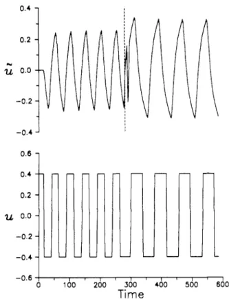
Noise).

This example is the same aa example 2 except that noise is injected between

K

and N (Figure 4). The level of the noise is set to be 5% of the amplitude of the limit cycle a. from the ideal relay feedback (w(t)

E

[-0.014,0.014]). From eq 19, if we assume m = 1, the hysteresis width c should be greater than 0.19.

Hysteresis width of 0.2 is taken in the second relay feedback experiment (after the dashed line in Figure 17).

Since m in this example is 1.45, which is quite close to the assumption, an additional experiment is not necessary.

0.9808 0.9806 0.9804 x d 0.9802 0.9800 0.9798 I 0.9708 0.9706 0.9704 x d 0.9702 0.9700 0.9698 Xdn'=O. 98 Xdn'=O.97 I I I I I 50 I b o 150 200 250 300 Time

Figure 15. Load responses for step change in feed flow rate (F) for the distillation example with two different operating conditione:

m1

= 0.98 and XTt = 0.97.

30f

25 0.98 0.97

s

A

I

&

Figure 16. Closed-loop log modulus (L,) over z domain for two operating conditions: XTt = 0.98 and XTt = 0.97.

The

L,,,

found is 10.49

dB,

which differs from the value from step-by-step searching by 0.53%. Again, very accurate approximation of

L,,,

can be found using the proposed procedure.

(10)

98 Ind. Eng. Chem. Res., Vol. 32, No. 1, 1993 0.6 0.4

1

! 0.2

-o,21

c

. . . . _: _I -0.4

1

-0.6

1

0.6 7 0.4 0.2 u 0.0 -0.2 -0.4 -0.6

'

I

6

160 260 300 460 5h 6do 760 8b

Figure 17. Relay feedback experiments for a system with noise.

1 8

Time

6. Conclusion

The monitoring procedure is an integral part of an intelligent control system. Most of the previously proposed monitoring procedures are based on the time domain analysis. A frequency domain monitoring procedure is proposed. The procedure is based on the relay feedback systems. With the linear assumption (eq 14), one can locate the maximum closed-loop log modulus (Le-) in two relay feedback experiments. The effectiveness of the proposed method is investigated, and the limitations are explored. The procedure is tested against linear systems, nonlinear distillation systems, and systems with and without noise. Simulation results show that it is extremely accurate in identifying

L,,,,

in an efficient manner. In addition to the autotuning feature, the proposed monitoring feature made intelligent control practical in the operating environment.

Acknowledgment

This

work is supported by the National Science Council of the ROC under Grant NSC 81-0402-E-011-07. We also thank S. H. Shen, who brought the clockwise Nyquist curve to our attention.

Nomenclature

a = amplitude of process oscillation

a. = amplitude of process oscillation for ideal relay al = amplitude of process oscillation for relay with hysteresis aN = amplitude of process oscillation corrupted with noise arg(.) = argument of

(-1

F = feed flow rate

F,,, = transformed IHclw,l (into t-domain)

f C ( < ) , f C K ( c ) = transformed a (into e-domain)

Go,) = process transfer function

h = relay haight

H,,,

= complementary sensitivity function

K,.,, = controller transfer function

K,, = ultimate gain

Lc = closed-loop log modulus

L , , , = maximum closed-loop log modulus

m = slope in the linear assumption (eq 14)

m N = slope in the linear assumption under noise m = monitoring mode

M = M-circle

N = describing function P = period of oscillation

P,

= ultimate period R = reflux flow rate

s = Laplace transform variable

u = input to the process (or output from the relay)

ii = controller output (or input to the relay)

w ( t ) = noise

Xd = distillate composition y = process output

Greek Symbols e = hysteresis

z = width of hysteresis giving

L,,,,

K =curvature

u = the bound of noise

wu = ultimate frequency

Appendix

From eqs 9 and 14, the frequency responses of the relay feedback system with linear assumption can be expressed as

GK

= Re

+

jIm (AI) where (A2) A Re = --[(me

+

ao)2

-

t2]-1/2 4h

According to the definition of the counterclockwise prop- erty, the curvature of GI&(Q) has to be positive (Tesi et al., 1992). This is

> O Refm

-

ReIm [Re2

+

Im2]3/2

K ( f j =

Then the derivatives with respect to e can be derived directly.

Re = --[(me

+

ao)2

-

e2]-1/2[e(m2

-

1)

+

mao]

Re = - - [ ( m e

+

ao)2

-

e2]-3/2(-[e(m2 - 1 ) 2

+

mao]2

+

il (A5) 4h 4h A (m2

-

l)[(mt

+

ao)2

-

t2]1 (A6) il Im = - - 4h fm =

o

Substituting eqs A5-A8 into eq A4, we have 2/3[(me

+

-

e2]-3/2 [t(m2

-

1)

+

rnaoI2

-

(m2

-

l)[(rnt

+

aOl2

-

t21 me

+

a. (me

+

~ [ ( m t

+

ao)2

-

t2]-3/2a02 (A9) For a relay feedback system, the amplitude of oscillation (me

+

ao) is always positive and greater than the width of hysteresis (e). Therefore,

(11)

I n d . Eng. Chem. Res. 1993, 32,99-107 99 Since GK,,, is counterclockwise,

GK,,,

has the clockwise

property (Figure 3).

Literature Cited

Arzcn, K. An Architecture for Expert System Based on Feedback Control. Automatica 1989, 25, 813.

Astrom, K. J.; Hagglund, T. Automatic Tuning of Simple Regulators with Specifications on Phase and Amplitude Margins. Automa-

tics 1984, 20, 645.

-

Astrom. K. J.: Handund. T. Automatic Tuning of PID Controllers: Instrument So&y of America: Researchkr’iangle Park, 1988. Astrom, K. J.; Anton, J. J.; A r z h , K. E. Expert Control. Automa-

tics 1986, 22, 227.

Chiang, R. C. Model Identification and On-Line Situation Analysis Based on Relay Feedback Systems. M.S. Thesis, National Taiwan Institute of Technology, Taipei, 1991 (in Chinese).

Chiang, R. C.; Shen, S. H.; Yu, C. C. Derivation of Transfer Function from Relay Feedback Systems. Ind. Eng. Chem. Res. 1992, 31, 855.

Doraiswami, R.; Jiang, J. Performance Monitoring in Expert Control Systems. Automatica 1989, 25, 799.

Francis, B. A. A Course in H, Control Theory. Lecture Notes in Control and Information Science 88; Springer-Verlag: Berlin, 1987.

Horowitz, I.; Ben-Adam, S. Clockwise Nature of Nyquist Locus of Stable Transfer Functions. Int. J. Control 1989, 49, 1433.

Luyben, W. L. Derivation of Transfer Function for Highly Non-linear Distillation Columns. Ind. Eng. Chem. Res. 1987, 26, 2495. Luyben, W. L. Process Modeling, Simulation and Control for

Chemical Engineers; McGraw-Hill: New York, 1990.

Morari, M.; Zafiriou, E. Robust Process Control; Prentice-Hall: Englewood Cliffs, NJ, 1989.

Ogata, K. Modern Control Engineering; Prentice-Hall: Englewood Cliffs, NJ, 1970.

Ortega, R.; Escobar, G.; Garcia, F. T o Tune or not to Tune?: A Monitoring Procedure to Decide. Automatica 1992,28, 179. Sastry, S.; Bodson, M. Adaptive Control: Stability, Convergence,

and Robustness; Prentice-Hall: Englewood Cliffs, NJ, 1989. Seborg, D. E.; Edgar, T. F.; Mellichamp, D. A. Process Dynamic and

Control; Wiley: New York, 1989.

Shen, S. H.; Yu, C. C. Indirect Feedforward Control: Multivariable Systems. Chem. Eng. Sci. 1992, 47, 3085.

Shih, Y. P. Process Control; You-Lin Publishing Co.: Tainan, 1982 (in Chinese).

Tesi, A.; Vicino, A.; Zappa, G. Clockwise Property of the Nyquist Plot with Implications for Absolute Stability. Automatica 1992, 28, 71.

Zames, G. Feedback and Optimal Sensitivity: Model Reference Transformations, Multiplicative Seminorms and Approximate Inverses. IEEE Trans. Autom. Control 1981, AC-26, 301.

Received f o r review April 13, 1992 Revised manuscript received September 9, 1992 Accepted October 5, 1992

Nonlinear Parameter Estimation for Real-Time Analytical Distillation

Models

Saibal Ganguly, Valluri Sairam,+ and Deoki

N.

Saraf*

Department of Chemical Engineering, Indian Institute of Technology, Kanpur 208016, India

Analytical process model based control is already a practical reality. The design of such controllers requires model parameter estimation for the nonlinear analytical process description, both under steady-state and dynamic conditions. Steady-state models of different degrees of complexity were examined and compared with experimental data from a pilot scale distillation column. While it is desirable

to

use a rigorous transport phenomena type model for understanding distillation

dynamics,

reduced order models offer several advantages. For real-time work, the use of dynamic optimization based on transient data provides a better scheme of parameter estimation. This algorithm, when used with the semirigorous model, provided the requisite speed and flexibility of utilizing noisy data without significant loss of accuracy. Nonlinear model predictive control of the top product composition of

a

pilot scale distillation column, using the proposed parameter estimation procedure, is cited as an example.

Introduction

Nonlinear parameter estimation has become an ap- pealing proposition with the advent of analytical model based controllers (Ganguly and Sard, 1992a; Riggs, 1990; Eaton and Rawlings, 1990; Moore and Corripio, 1990; etc.). The transport phenomena type analytical models are also

useful in understanding process dynamics, design of experiments, and operator training. These are superior to empirical models since the former provide an insight into the physics of the process whereas the latter treat it as a black box. Moreover, extrapolation can be made with greater confidence while using analytical models which is strictly prohibited with empirical ones.

It is seldom possible to provide a complete analytical description of a process, however simple it may be. In the case of distillation columns, there are several phenomena such as deviation of tray behavior from the ideal equilib-

*

To whom correspondence should be addressed.

Present addreas: R&D Center, Engineers India Ltd., Gurgaon, India.

o w m a 5 1931 2632-0099~04.00 J O

rium stage, role of residence time, etc., which are not amenable to modeling in terms of simple equations. While researchers are still trying to model these aspects in terms of physical quantities, from a practical viewpoint, one uses parameters such as stage efficiencies in the model which are back-calculated so as to match the model predictions with the experimental observations in the least squared sense. The measured process data, from which the parameters are estimated, are often contaminated with process noise, instrument error, and unmodeled changing process characteristics. For dynamic description, therefore, some additional adjustable parameters may be required. Choice of these parameters and their estimation is by no means a simple task and is the topic of discussion in this paper.

In this study, model parameters have been estimated for available rigorous, reduced order, and semirigorous models in order to match their predictions with the experimental data from a pilot scale distillation column. Two types of transients, which are commonly encountered in the operation of a distillation column, have been examined. One is during switchover from one steady-state condition

Monitoring procedure for intelligent control: on-line identification of maximum closed-loop log modulus