國立交通大學
統計學研究所
碩 士 論 文
多 重 假 設 檢 定 問 題 下
t
統 計 量 的 行 為
Behavior of
t
-statistic in Multiple Hypothesis
Testing Problem
研 究 生:王怡倫
指導教授:洪慧念 博士
多 重 假 設 檢 定 問 題 下
t
統 計 量 的 行 為
Behavior of
t
-statistic in Multiple Hypothesis
Testing Problem
研 究 生:王怡倫 Student : Yi-Lun Wang
指導教授:洪慧念 Advisor : Dr. Hui-Nien Hun
g
國 立 交 通 大 學
統計學研究所
碩 士 論 文
A Thesis
Submitted to Institute of Statistics College of Science
National Chiao Tung University
in Partial Fulfillment of the Requirements for the Degree of
Master in Statistics
June 2009
Hsinchu,Taiwan, Republic of China
多 重 假 設 檢 定 問 題 下 統 計 量 的 行 為
t
研究生:王怡倫 指導教授:洪慧念博士
國 立 交 通 大 學 統 計 學 研 究 所
摘 要
在基因晶片資料的分析中,通常我們會同時考慮數以千計或數萬
個
t
-檢定統計量用以區別個別基因之重要性。在這種多重檢定的過
程中,這些檢定統計量常常會存在一些相關性,因此他們的分配將不
會是一般的常用的
t
分配。在這篇論文,我們討論這許多
t
-檢定統
計量的分配不為
t
分配的可能原因。這些可能原因分別是不同基因間
存在某些相關,不同基因晶片間存在某些相關,以及基因表現不是來
自常態分配的假設。在分析的過程中,我們會考慮一些特殊模型並且
運用統計模擬分析之技巧來探討這些可能原因的影響。
關 鍵 字 : 多 重 檢 定 過 程 ,
t
-檢 定 量 ,
t
-分 配
Behavior of t-statistic in Multiple Hypothesis
Testing Problem
Student: Yi-Lun Wang
Advisor: Dr. Hui-Nien Hung
Institute of Statistics
National Chiao Tung University
Abstract
Microarray data has been studied widely, with thousands or even millions of test statistics ti’s to be considered at the same time. These test statistics ti’s are
correlated or not regular distributed on multiple testing procedure. In this pa-per, we discussed three possible reasons for the distribution of test statistics ti’s
differing from t-distribution. The three reasons are correlation between genes, correlation among microarrays, and various distribution assumptions. Then, we consider several models and conclude that correlation among microarrays and various distribution assumptions are most important effects which make the dis-tribution of test statistics ti’s differing from t-distribution.
誌 謝
這 篇 論 文 能 順 利 的 完 成 , 首 先 要 感 謝 洪 慧 念 教 授 , 謝 謝 老 師 對 這 篇 論 文辛 勤
的 指 導 與 批 閱。感 謝 老 師 在 課 業 上 適 時 的 給 予 我 建 議 和 鼓 勵 並 且 教 導 我 一 些 人 生 的 道 理 , 讓 我 受 益 良 多 。 同 時 , 也 感 謝 口 試 委 員 提 供 諸 多 建 議 , 使 得 本 論 文 更 加 完 善 。 再 來 要 感 謝 郃 嵐 學 姐 的 鼓 勵 和 幫 助 , 謝 謝 你 協 助 我 很 多 生 活 或 課 業 上 的 問 題 。 還 有 感 謝 班 上 的 同 學 及 身 旁 的 朋 友 , 謝 謝 你 們 給 予 我 課 業 和 生 活 上 的 幫 助 , 因 為 有 你 們 的 參 與 , 我 的 研 究 所 生 涯 才 有 難 忘 的 回 憶 。 最 後 , 感 謝 我 的 父 母 親 , 讓 我 在 求 學 過 程 中 能 將 心 力 都 放 在 課 業 上 , 謝 謝 他 們 辛 苦 的 栽 培 。 僅 將 此 論 文 獻 給 我 最 敬 愛 的 父 母 親 、 洪 慧 念 教 授 及 所 有 在 周 圍 關 心 我 的 人 , 謝 謝 大 家 。 王 怡 倫 謹 誌 于 國 立 交 通 大 學 統 計 學 研 究 所 中 華 民 國 九 十 八 年 六 月Abstract(in Chinese). . . i
Abstract(in English). . . ii
Acknowledgements(in Chinese) . . . iii
Contents
1 Introduction 1 2 Literature Review 2 2.1 Multiple Hypothesis Testing in a Microarray Experiment . . . 22.2 Microarray Experiments . . . 4
2.2.1 The Breast Cancer Study . . . 4
2.2.2 The HIV Study . . . 4
3 The Empirical Distribution of the zi’s 7 4 The Models and Simulation Study 8 4.1 Models of correlation between genes . . . 9
4.1.1 Model 1 . . . 9
4.1.2 Model 2 . . . 9
4.1.3 Model 3 . . . 11
4.2 Models of correlation among microarrays . . . 12
4.2.1 Model 4 . . . 12
4.2.2 Model 5 . . . 13
4.2.3 Model 6 . . . 14
4.3 Various Distribution Assumptions . . . 15
4.3.1 Model 7 . . . 15 4.3.2 Model 8 . . . 16 4.3.3 Model 9 . . . 16 4.3.4 Model 10 . . . 17 4.3.5 Model 11 . . . 17 4.3.6 Model 12 . . . 18 4.4 Results of Simulation . . . 19 5 Real Data 20 6 Conclusions and Future Research 22
List of Figures
1 Histograms of z-Values From Two Microarray Experiments. (a) Breast cancer study, 3226 genes. (b) HIV study, 7680 genes. (This figure and
descriptions are quoted from Efron (2007)). . . 6
2 The distribution of the zi’s between genes plot. . . 10
3 The distribution of the zi’s between genes plot. . . 11
4 The distribution of the zi’s between genes plot. . . 12
5 The distribution of the zi’s among microarrays plot. . . 13
6 The distribution of the zi’s among microarrays plot. . . 14
7 The distribution of the zi’s among microarrays plot. . . 15
8 The distribution of the zi’s under various distribution assumption plot. 16 9 The distribution of the zi’s under various distribution assumption plot. 17 10 The distribution of the zi’s under various distribution assumption plot. 18 11 The distribution of the zi’s plot in real data. . . 21
1
Introduction
The microarray data in biomedical research has been studied extensively in the past few years. Microarray is a technology to detect mRNA expression level. In general, detecting mRNA expression level can help identify genes that contribute to disease. That is, the goal of a microarray experiment is to identify those genes that are differen-tially expressed within different samples. Besides, the number of samples we observed is much less than the number of genes in a microarray experiment, thus generating a large-scale multiple hypothesis testing problem (Gentleman, Carey, Huber, Irizarry, and Dudoit, 2005; Efron, 2007).
A large-scale multiple hypothesis testing problem in a microarray experiment in-volves the simultaneous test of thousands, or even millions, of null hypotheses (Gen-tleman et al., 2005). Usually we use two-sample t-statistics ti comparing expression
levels under two different conditions for m genes. Then, the ti’s are transformed to
zi’s such that, under normal assumption, zi has a standard normal distribution (Efron,
2007). Efron (2007) displayed two histograms of zi’s from two microarray experiments
and described the zi’s correlations can cause the fact that the distribution of the zi’s
differs from N(0,1), called theoretical null distribution.
Since the earlier study did not focus on the reason of the histograms of zi’s differing
from N(0,1) on multiple testing procedures. Hence, in this paper, we have two pur-poses: (a) to discuss the possible reasons for the distribution of the zi’s differing from
N(0,1); (b) to simulate the data from the possible models and recommend the possible reasons in large-scale multiple hypothesis testing problem. The paper is organized as follows. Section 2 reviews the multiple hypothesis testing problem in a microarray ex-periment or two microarray exex-periments: the breast cancer study and the HIV study. Moreover, Section 3 discusses the possible reasons for over-diversion of the distribution of the zi’s in the breast cancer study and over-converge of the distribution of the zi’s in
the HIV study. In Section 4, we study possible models of gene expression data. Section 5 uses the real data in multiple hypothesis testing and makes some comments. Finally, Section 6 concludes the paper with a brief summary and discusses the future work.
2
Literature Review
2.1
Multiple Hypothesis Testing in a Microarray Experiment
Suppose we have a microarray experiment which produces gene expression data on m genes (i.e., variables or features) for n mRNA samples (i.e., observations or microarrays or patients). Then the gene expression levels may be summarized by a m × n matrix X = (xij), where xij denotes the expression measures of gene i and sample j. The
rows i = 1, . . . , m represent the prob sets (genes) and the columns j = 1, . . . , n rep-resent the different microarrays (samples). The gene expression levels might be either absolute (e.g., Affymetrix oligonucleotide arrays (Lockhart et al., 1996; Dudoit, Shaffer and Boldrick, 2003)) or relative to the expression levels of a suitably defined common reference sample (e.g. two-color cDNA microarrays (Dudoit et al., 2003)).
In a microarray experiment, the number m is usual several thousands or even mil-lions and the number n is usual anywhere between around eight and a few hundreds. In a typical experiment, the n samples would consist of n1 treatment samples and n2
con-trol samples, for example, the treatment samples are patients with BRCA1 mutations and the control samples are patients with BRCA2 mutations in breast cancer study. The goal of a microarray experiment is to identify those genes that are differentially expressed in the different mutations of breast cancer. Therefore, suppose the single test is considered for each gene, the null hypothesis for testing that the gene i has the same expression distribution under two different conditions. For tests of means, the test statistic is the usual two-sample t-statistic, where the two-sample t-statistic depends on the standard t-test (equal variance) or Welch t-test (unequal variance). Thus, we have m null hypotheses to consider simultaneously, each with its own test statistic,
Null hypothesis : H1, H2, . . . , Hi, . . . , Hm
Test statistic : t1, t2, . . . , ti, . . . , tm.
Then, we transform ti to a zi such that, under normal assumption, zi has a standard
normal distribution and derive rejection regions (Gentleman et al., 2005). The adjusted p-value for null hypotheses is defined as the smallest type I error, α (e.g., FWER or
FDR (Benjamini and Hochberg, 1995; Dudoit et al., 2003; Efron, 2004, 2005, 2006, 2007; Ge, Dudoit, and Speed, 2003)), at which one would reject Hi (Gentleman et al.,
2005) in the multiple hypothesis testing problem. Finally, we reject the null hypotheses if the adjusted p-value is smaller than α (Dudoit et al., 2003; Ge et al., 2003; Gentleman et al., 2005). That is to say, we reject the Hi, means that the gene i is differentially
expressed under two different mutations of breast cancer. The procedure of the several tests with controlled in type I error is called a multiple testing procedure, abbreviated MTP (Dudoit et al., 2003; Ge et al., 2003; Gentleman et al., 2005).
It is noteworthy that Benjamini and Hochberg (1995) defined the FDR to be the expected proportion of true null hypotheses among the rejected hypotheses, FDR = E(V/R), where V denote the number of rejecting H0 under H0 is true and R denote
the number of rejecting H0 in all hypotheses. Besides, Efron et al. (2001) and Efron
(2004) described that local false discovery rate, fdr(z)=f0(z)/f (z), is closely related to
Benjamini and Hochberg’s FDR criterion. The density f0(z) is null probability density
function (e.g., theoretical, empirical, or permutation null hypothesis distribution) and the density f (z) is probability density function derived from the empirical distribution of the zi’s (Efron, 2004; Efron et al., 2001)). Moreover, Efron (2004) report that we
can find out the genes which are differentially expressed by the local fdr. The details about local fdr are described in Efron (2004) and Efron et al. (2001).
The choice of null distribution (e.g., theoretical, empirical, or permutation null hypothesis distribution) is important to control the local fdr (Efron 2004, 2006, 2007; Gentleman et al., 2005). Different choices may influence the conclusion on identifying which genes as differential or the same in the multiple hypothesis testing (Efron 2004, 2006, 2007; Gentleman et al., 2005). Efron (2004) reported that the appropriate choice of null distribution is the empirical null rather than the theoretical null or permutation null in some microarray experiments. Also, Efron (2006) suggested that the theoretical null or permutation null is inappropriate null in HIV study since the theoretical null or permutation null may make there is no differential genes on MTP (Efron, 2006). Hence, we need to select a suitable distribution in multiple hypothesis testing under
different microarray experiments.
2.2
Microarray Experiments
For the microarray experiments, we consider the breast cancer study and the HIV study below.
2.2.1 The Breast Cancer Study
Hedenfalk, Duggen, Chen, et al. (2001) reported on a microarray experiment con-cerning the mutant genes of hereditary breast cancer. It is known that two different mutations, BRCA1 and BRCA2, lead to greatly increased breast cancer risk.
The experiment included 15 breast cancer patients, 7 from BRCA1 mutation pa-tients and 8 from BRCA2. Each patient measured a microarray of expression levels for the same m = 3226 genes. Then, we have a m × n matrix X = (xij) for the
breast cancer study, where m = 3226 rows denote genes and n = 15 columns denote microarrays. Each row of X (i.e., gene) yielded a two-sample t-statistic ti comparing
BRCA1 with BRCA2 patients, which was then transformed to a zi.
zi = Φ−1(G0(ti)), i = 1, 2, ..., m,
where Φ is the standard normal cumulative distribution function (c.d.f.), and G0 is the
c.d.f. of a standard Student’s t distribution with 13 degrees of freedom. Hence, we get m = 3226 test statistic zi’s and the distribution of the zi’s are displayed in Figure 1(a)
(Efron, 2004, 2005, 2007; Gottardo, Raftery, Yeung, and Bumgarner, 2006). 2.2.2 The HIV Study
The human immunodeficiency virus (HIV) study, described by van’t Wout et al. (2003), contained 8 samples, 4 from HIV-positive patients and 4 from HIV-negative controls. Each samples measured a microarray of expression levels for the same m = 7680 genes. Then, we have a m × n matrix X = (xij) for the HIV study, where m = 7680 rows
a two-sample t-statistic ticomparing HIV-positive patients with HIV-negative controls,
which was then transformed to a zi.
zi = Φ−1(G0(ti)), i = 1, 2, ..., m,
where Φ is the standard normal c.d.f., and G0 is the c.d.f. of a standard Student’s t
distribution with 6 degrees of freedom. Hence, we get m = 7680 test statistic zi’s and
the distribution of the zi’s are displayed in Figure 1(b) (Efron, 2004, 2005, 2006, 2007;
Gottardo et al., 2006).
The data from the breast cancer study and the HIV study were two-color cDNA microarrays and people make quality assessment and preprocessing (e.g. normaliza-tion) for the data before using them in multiple hypothesis testing (Dudoit et al., 2003; Gottardo et al., 2006; Gentleman et al., 2005).
Efron (2007) described that we usually presuppose most of the genes to be null in microarray experiments, the goal being to identify some significant nonnull genes. Therefore, we expect zi to have closely a standard normal distribution for null genes
(Efron, 2007). In other words, under null hypothesis, zi should have a standard normal
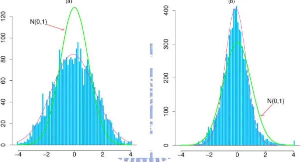
distribution if gene i has the same expression distribution for BRCA1 and BRCA2 pa-tients or for HIV-positive papa-tients and HIV-negative controls. Efron (2007) reported that heavy curves indicate N(0,1) theoretical null densities and light curves indicate empirical null densities fit to central z-values in Figure 1, as done by Efron (2004). However, the histograms of z-values in Figure 1, where the distribution of the zi’s from
breast cancer is wider than N(0,1) and from HIV study is narrower than N(0,1) (Efron, 2006, 2007). Efron (2007) pointed out that the correlations in multiple hypothesis testing can make the observed all zi’s behave as N(0, σ2), where σ is obviously
dif-ferent than 1. Next section, we will discuss the correlation and other reasons for this phenomenon.
Figure 1: Histograms of z-Values From Two Microarray Experiments. (a) Breast cancer study, 3226 genes. (b) HIV study, 7680 genes. (This figure and descriptions are quoted from Efron (2007)).
3
The Empirical Distribution of the z
i’s
In this section, we discuss the possible reasons which caused the distribution of the zi’s
that obviously differs from the N(0,1) in microarray experiments. First, Efron (2007) indicated that there were some gene correlations in the breast cancer data and in the HIV data. Besides, the disease is caused by abnormal genes and there are essential correlations between genes in biology. Hence we may say that there are gene correlation structures in the breast cancer data and the HIV data.
Secondly, Hedenfalk et al. (2001) pointed out that these patients with primary breast cancer and who had a family history of breast or ovarian cancer or both were asked to provide a blood sample for BRCA1 and BRCA2 mutations in the genetic breast cancer. If some of the patients are come from the same family, some of their gene may correlate. Hence the patients may correlate with the relationship of relatives. Furthermore, Efron (2004) indicated that the first four and the last four microarrays in the BRCA2 patients were mutually correlated. Moreover, since the HIV is a rare disease, the HIV patients usually have the same features, for example, the patients are homosexuality, drug addicts and infected with mother. According to the above, we may safely say that there are the correlation structures among patients (i.e. microarrays ). Finally, if the data (xij) are independent and identically distributed (i.i.d.) random
variables from normal distribution, we may apply the two-sample t-statistic in multiple hypothesis testing. In other words, if the data (xij) are independent and identically
distributed (i.i.d.) random variables from other distributions, the two-sample t-statistic may not have the t-distribution.
Hence, as mentioned above, we may consider the three possible reasons under the following items : (1) correlation between genes. (2) correlation among microarrays. (3) various distribution assumptions. In the next section, we discuss further the models of these possible reasons. Besides, we apply these models for simulating data and then compare the results of the simulation.
4
The Models and Simulation Study
For generating dependent data, we consider two kinds of time series models: the au-toregressive model (AR) and the moving average model (MA). We introduce the AR model and the MA model.
Definition 1 An autoregressive model of order p, abbreviated AR(p), is defined to be
Xt= φ1Xt−1+ φ2Xt−2+ ... + φpXt−p+ Zt,
where Xt is stationary, φ1, φ2, ..., φp (φp 6= 0) are constants, and Zt is a Gaussian white
noise series with mean 0 and variance σ2 (Chan, 2001; Shumway, and Stoffer, 2005).
Definition 2 A moving average model of order q, abbreviated MA(q), is defined to be
Xt= Zt+ θ1Zt−1+ θ2Zt−2+ ... + θqZt−q,
where there are q lags in the moving average, θ1, θ2, ..., θq (θq 6= 0) are constants, and Zt
is a Gaussian white noise series with mean 0 and variance σ2 (Chan, 2001; Shumway, and Stoffer, 2005).
Suppose a microarray experiment includes n (n = n1 + n2) patients, n1 from
group 1 and n2 from group 2. Each patient measures a microarray of expression levels
for the same m genes. We want to identify those genes that are differentially expressed under the two group. Let X = (xij) represent gene expression and be a m × n matrix,
where i = 1, ..., m denotes genes and j = 1, ..., n (n = n1+ n2) denotes microarrays.
In the simulation study, we choose m = 100000 genes and n = 14 (n1 = n2 = 7)
micrarrays. Then we apply the data on the multiple testing procedures. Therefore, we get m = 100000 zi’s. In Figure 2∼10, we plot the empirical distribution of the zi’s of
characteristics of the data are described below.
4.1
Models of correlation between genes
In the following models, we consider that there is some correlation between genes, but there is no dependence between microarrays.
4.1.1 Model 1
For model 1, we consider (
xi1, xi2, ..., xin1 ∼ i.i.d. N (0, σ
2)
xin1+1, xin1+2, ..., xin ∼ i.i.d. N (0, σ
2), x1j, x2j, ..., xmj ∼ AR(p),
where each gene follows a normal distribution with mean 0 and variance σ2, and each
microarray follows an AR(p) model. The elements from different microarrays are in-dependent and from different genes have the AR(p) correlation structures. For exam-ple, take p = 2, the x1j, x2j, ..., xmj ∼ AR(2), i.e., xtj = φ1xt−1j + φ2xt−2j + zt, t =
1, ..., m. The coefficients, φ1-value and φ2-value, represent the size of correlation among
xtj, xt−1j, and xt−2j, t = 1, ..., m. The larger the φ1 (or φ2) is, the larger the correlation
is.
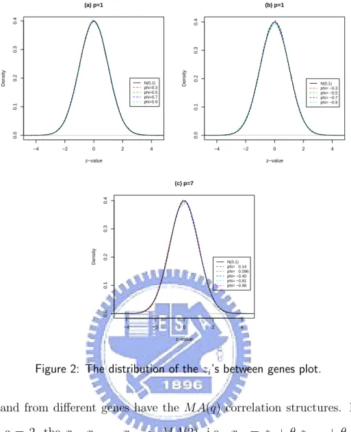
Figure 2(a) displays the empirical distribution of the zi’s of the model 1 with φ1 =
0.3, 0.5, 0.7, 0.9 as p = 1. Figure 2(b) displays the empirical distribution of the zi’s of
the model 1 with φ1 = -0.3, -0.5, -0.7, -0.9 as p = 1. Figure 2(c) displays the empirical
distribution of the zi’s of the model 1 with φ1 = ... = φ7 = 0.14, 0.096, -0.40, -0.81,
-0.96 as p = 7. 4.1.2 Model 2
For model 2, we consider (
xi1, xi2, ..., xin1 ∼ i.i.d. N (0, σ
2)
xin1+1, xin1+2, ..., xin ∼ i.i.d. N (0, σ
2), x1j, x2j, ..., xmj ∼ M A(q),
where each gene follows a normal distribution with mean 0 and variance σ2, and each
inde-−4 −2 0 2 4 0.0 0.1 0.2 0.3 0.4 (a) p=1 z−value Density N(0,1) phi=0.3 phi=0.5 phi=0.7 phi=0.9 −4 −2 0 2 4 0.0 0.1 0.2 0.3 0.4 (b) p=1 z−value Density N(0,1) phi= −0.3 phi= −0.5 phi= −0.7 phi= −0.9 −4 −2 0 2 4 0.0 0.1 0.2 0.3 0.4 (c) p=7 z−value Density N(0,1) phi= 0.14 phi= 0.096 phi= −0.40 phi= −0.81 phi= −0.96
Figure 2: The distribution of the zi’s between genes plot.
pendent and from different genes have the M A(q) correlation structures. For exam-ple, take q = 2, the x1j, x2j, ..., xmj ∼ M A(2), i.e., xtj = zt + θ1zt−1j + θ2zt−2j, t =
1, ..., m. The coefficients, θ1 and θ2, represent the size of correlation among zt, zt−1j,
and zt−2j, t = 1, ..., m. The larger the θ1 (or θ2) is, the larger the correlation is.
Figure 3(a) displays the empirical distribution of the zi’s of the model 2 with θ1
= 0.1, 0.3, 0.5, 0.9 as q = 1. Figure 3(b) displays the empirical distribution of the zi’s of the model 2 with θ1 = -0.1, -0.3, -0.5, -0.9 as q = 1. Figure 3(c) displays the
empirical distribution of the zi’s of the model 2 with θ1 = ... = θ7 = 0.1, 0.3, 0.5, 0.9
as q = 7. Figure 3(d) displays the empirical distribution of the zi’s of the model 2 with
−4 −2 0 2 4 0.0 0.1 0.2 0.3 0.4 (a) q=1 z−value Density N(0,1) theta=0.1 theta=0.3 theta=0.5 theta=0.9 −4 −2 0 2 4 0.0 0.1 0.2 0.3 0.4 (b) q=1 z−value Density N(0,1) theta= −0.1 theta= −0.3 theta= −0.5 theta= −0.9 −4 −2 0 2 4 0.0 0.1 0.2 0.3 0.4 (c) q=7 z−value Density N(0,1) theta=0.1 theta=0.3 theta=0.5 theta=0.9 −4 −2 0 2 4 0.0 0.1 0.2 0.3 0.4 (d) q=7 z−value Density N(0,1) theta= −0.1 theta= −0.3 theta= −0.5 theta= −0.9
Figure 3: The distribution of the zi’s between genes plot.
4.1.3 Model 3
Qiu, Brooks, Klebanov, and Yakovlev (2005a) suggested the model 3 which has an exchangeable correlation structure between genes. For model 3, we consider
( xi1, xi2, ..., xin1 ∼ i.i.d. N (0, σ 2) xin1+1, xin1+2, ..., xin ∼ i.i.d. N (0, σ 2), cor(xkj, xlj) = c, k = 1, ..., m, j = 1, ..., m , k 6= l,
where each gene follows a normal distribution with mean 0 and variance σ2. The
elements from different microarrays are independent and the correlation coefficient between any two elements xij of the same microarray is equal to c, where c is between
0 and 1 (Qiu et al., 2005a).
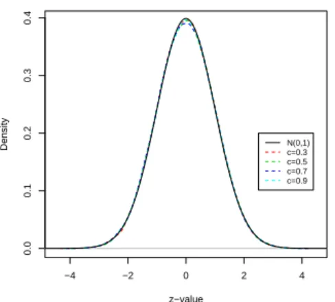
Figure 4 displays the empirical distribution of the zi’s of the model 3 with c = 0.3,
−4 −2 0 2 4 0.0 0.1 0.2 0.3 0.4 z−value Density N(0,1)c=0.3 c=0.5 c=0.7 c=0.9
Figure 4: The distribution of the zi’s between genes plot.
4.2
Models of correlation among microarrays
In the following models, we consider that there is some correlation between microarrays, but there is no dependence between genes.
4.2.1 Model 4
For model 4, we consider
x1j, x2j, ..., xmj ∼ i.i.d. N (0, σ2),
(
xi1, xi2, ..., xin1 ∼ AR(p)
xin1+1, xin1+2, ..., xin∼ AR(p),
where each microarray follows a normal distribution with mean 0 and variance σ2, and each gene follows an AR(p) model. The elements from different genes are independent and from different microarrays have the AR(p) correlation structures. For example, take p = 2, the xi1, xi2, ..., xin1 ∼ AR(2) and the xin1+1, xin1+2, ..., xin ∼ AR(2), i.e.,
xit= φ1xit−1+ φ2xit−2+ zt, t = 1, ..., n. The coefficients, φ1 and φ2, represent the size
of correlation among xit, xit−1, and xit−2, t = 1, ..., n. The larger the φ1 (or φ2) is, the
larger the correlation is.
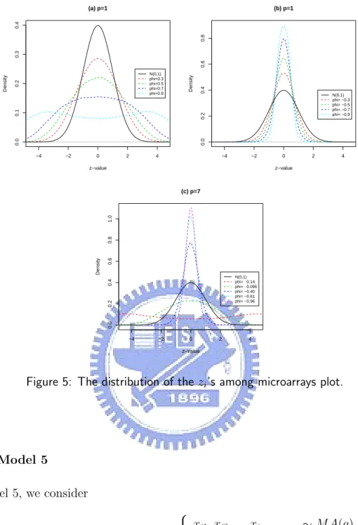
Figure 5(a) displays the empirical distribution of the zi’s of the model 4 with φ1 =
0.3, 0.5, 0.7, 0.9 as p = 1. Figure 5(b) displays the empirical distribution of the zi’s of
the model 4 with φ1 = -0.3, -0.5, -0.7, -0.9 as p = 1. Figure 5(c) displays the empirical
distribution of the zi’s of the model 4 with φ1 = ... = φ7 = 0.14, 0.096, -0.40, -0.81,
−4 −2 0 2 4 0.0 0.1 0.2 0.3 0.4 (a) p=1 z−value Density N(0,1) phi=0.3 phi=0.5 phi=0.7 phi=0.9 −4 −2 0 2 4 0.0 0.2 0.4 0.6 0.8 (b) p=1 z−value Density N(0,1) phi= −0.3 phi= −0.5 phi= −0.7 phi= −0.9 −4 −2 0 2 4 0.0 0.2 0.4 0.6 0.8 1.0 (c) p=7 z−value Density N(0,1) phi= 0.14 phi= 0.096 phi= −0.40 phi= −0.81 phi= −0.96
Figure 5: The distribution of the zi’s among microarrays plot.
4.2.2 Model 5
For model 5, we consider
x1j, x2j, ..., xmj ∼ i.i.d. N (0, σ2),
(
xi1, xi2, ..., xin1 ∼ M A(q)
xin1+1, xin1+2, ..., xin∼ M A(q),
where each microarray follows a normal distribution with mean 0 and variance σ2, and
each gene follows a M A(q) model. The elements from different genes are independent and from different microarrays have the M A(q) correlation structures. For example, take q = 2, the xi1, xi2, ..., xin1 ∼ M A(2) and the xin1+1, xin1+2, ..., xin ∼ M A(2), i.e.,
xit = zt+ θ1zit−1+ θ2zit−2, t = 1, ..., n. The coefficients, θ1 and θ2, represent the size
of correlation among zt, zit−1, and zit−2, t = 1, ..., n. The larger the θ1 (or θ2) is, the
−4 −2 0 2 4 0.0 0.1 0.2 0.3 0.4 (a) q=1 z−value Density N(0,1) theta=0.1 theta=0.3 theta=0.5 theta=0.9 −4 −2 0 2 4 0.0 0.2 0.4 0.6 0.8 1.0 (b) q=1 z−value Density N(0,1) theta= −0.1 theta= −0.3 theta= −0.5 theta= −0.9 −4 −2 0 2 4 0.0 0.1 0.2 0.3 0.4 (c) q=7 z−value Density N(0,1) theta=0.1 theta=0.3 theta=0.5 theta=0.9 −4 −2 0 2 4 0.0 0.1 0.2 0.3 0.4 0.5 (d) q=7 z−value Density N(0,1) theta= −0.03 theta= −0.05 theta= −0.07 theta= −0.1
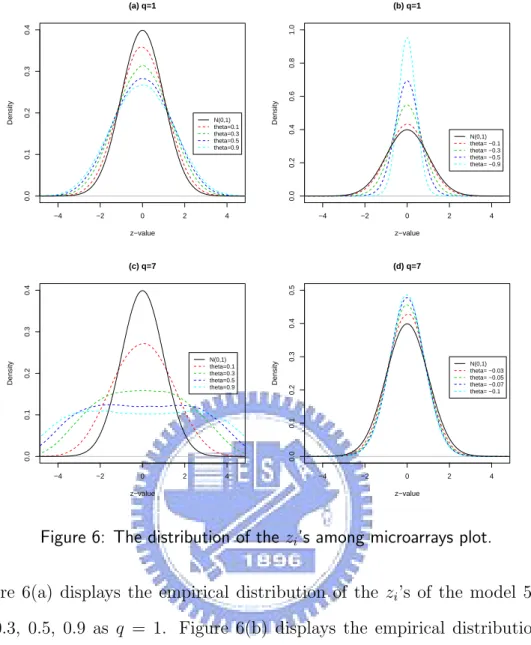
Figure 6: The distribution of the zi’s among microarrays plot.
Figure 6(a) displays the empirical distribution of the zi’s of the model 5 with θ1
= 0.1, 0.3, 0.5, 0.9 as q = 1. Figure 6(b) displays the empirical distribution of the zi’s of the model 5 with θ1 = -0.1, -0.3, -0.5, -0.9 as q = 1. Figure 6(c) displays the
empirical distribution of the zi’s of the model 5 with θ1 = ... = θ7 = 0.1, 0.3, 0.5, 0.9
as q = 7. Figure 6(d) displays the empirical distribution of the zi’s of the model 5 with
θ1 = ... = θ7= -0.03, -0.05, -0.07, -0.1 as q = 7.
4.2.3 Model 6
The model 6 has an exchangeable correlation structure among microarrays. For model 6, we consider
x1j, x2j, ..., xmj ∼ i.i.d. N (0, σ2),
(
cor(xik, xil) = c, k = 1, ..., n1, j = 1, ..., n1, k 6= l
−4 −2 0 2 4 0.0 0.1 0.2 0.3 0.4 z−value Density N(0,1) c=0.3 c=0.5 c=0.7 c=0.9
Figure 7: The distribution of the zi’s among microarrays plot.
where each microarray follows a normal distribution with mean 0 and variance σ2. The
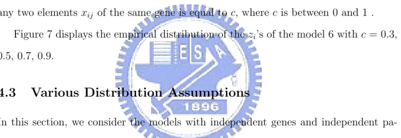
elements from different genes are independent and the correlation coefficient between any two elements xij of the same gene is equal to c, where c is between 0 and 1 .
Figure 7 displays the empirical distribution of the zi’s of the model 6 with c = 0.3,
0.5, 0.7, 0.9.
4.3
Various Distribution Assumptions
In this section, we consider the models with independent genes and independent pa-tients. But, the empirical distribution of genes are not normal.
4.3.1 Model 7
For model 7, we consider (
xi1, xi2, ..., xin1 ∼ i.i.d. Gamma(α = shape, λ = rate),
xin1+1, xin1+2, ..., xin ∼ i.i.d. Gamma(α = shape, λ = rate),
where the independent and identically distributed random variables xij are generated
from a gamma distribution with mean α/λ and variance α/λ2.
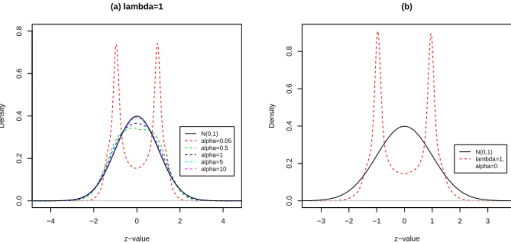
Figure 8(a) displays the empirical distribution of the zi’s of the model 7 with α =
−4 −2 0 2 4 0.0 0.2 0.4 0.6 0.8 (a) lambda=1 z−value Density N(0,1) alpha=0.05 alpha=0.5 alpha=1 alpha=5 alpha=10 −3 −2 −1 0 1 2 3 0.0 0.2 0.4 0.6 0.8 (b) z−value Density N(0,1) lambda=1, alpha=0
Figure 8: The distribution of the zi’s under various distribution assumption plot.
4.3.2 Model 8
For model 8, we consider (
xi1, xi2, ..., xin1 ∼ i.i.d. Cauchy(α = location, λ = scale)
xin1+1, xin1+2, ..., xin ∼ i.i.d. Cauchy(α = location, λ = scale),
where the independent and identically distributed random variables xij are generated
from a cauchy distribution with location α and scale λ.
Figure 8(b) displays the empirical distribution of the zi’s of the model 8 with λ =
1, α = 0.
4.3.3 Model 9
For model 9, we consider (
xi1, xi2, ..., xin1 ∼ i.i.d. W eibull(λ = shape, α = scale, β = location)
xin1+1, xin1+2, ..., xin ∼ i.i.d. W eibull(λ = shape, α = scale, β = location),
where the independent and identically distributed random variables xij are generated
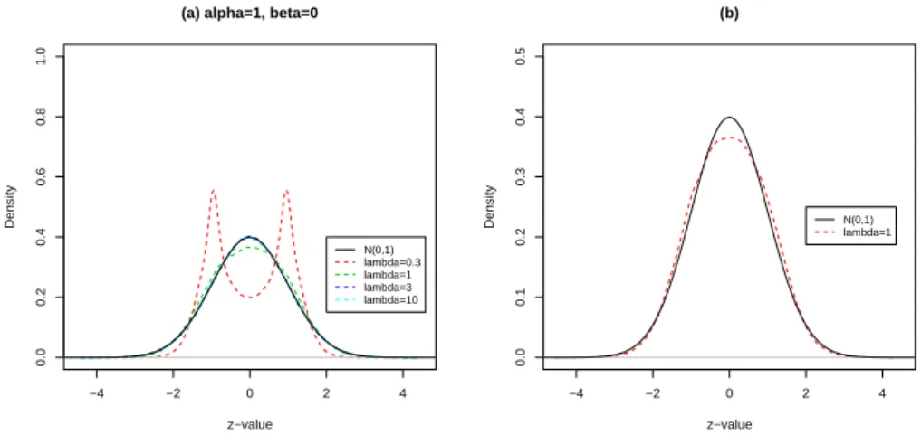
from a weibull distribution with mean β + αΓ(1 + 1/λ) and variance α2(Γ(1 + 2/λ) −
(Γ(1 + 1/λ))2).
Figure 9(a) displays the empirical distribution of the zi’s of the model 9 with λ =
−4 −2 0 2 4 0.0 0.2 0.4 0.6 0.8 1.0
(a) alpha=1, beta=0
z−value Density N(0,1) lambda=0.3 lambda=1 lambda=3 lambda=10 −4 −2 0 2 4 0.0 0.1 0.2 0.3 0.4 0.5 (b) z−value Density N(0,1) lambda=1
Figure 9: The distribution of the zi’s under various distribution assumption plot.
4.3.4 Model 10
For model 10, we consider (
xi1, xi2, ..., xin1 ∼ i.i.d. Exp(λ = rate)
xin1+1, xin1+2, ..., xin ∼ i.i.d. Exp(λ = rate),
where the independent and identically distributed random variables xij are generated
from an exponential distribution with mean 1/λ and variance 1/λ2.
Figure 9(b) displays the empirical distribution of the zi’s of the model 10 with λ =
1.
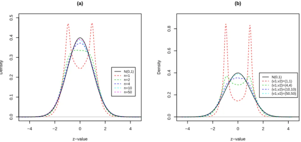
4.3.5 Model 11
For model 11, we consider (
xi1, xi2, ..., xin1 ∼ i.i.d. t(n = degrees of f reedom)
xin1+1, xin1+2, ..., xin ∼ i.i.d. t(n = degrees of f reedom),
where the independent and identically distributed random variables xij are generated
from a t distribution with mean 0 (n > 1) and variance n/(n − 2) (n > 2).
Figure 10(a) displays the empirical distribution of the zi’s of the model 11 with n
−4 −2 0 2 4 0.0 0.1 0.2 0.3 0.4 0.5 (a) z−value Density N(0,1) n=1 n=2 n=4 n=10 n=50 −4 −2 0 2 4 0.0 0.2 0.4 0.6 0.8 (b) z−value Density N(0,1) (v1,v2)=(1,1) (v1,v2)=(4,4) (v1,v2)=(10,10) (v1,v2)=(50,50)
Figure 10: The distribution of the zi’s under various distribution assumption plot.
4.3.6 Model 12
For model 12, we consider (
xi1, xi2, ..., xin1 ∼ i.i.d. F (v1, v2)(v1, v2 = degrees of f reedom)
xin1+1, xin1+2, ..., xin ∼ i.i.d. F (v1, v2)(v1, v2 = degrees of f reedom),
where the independent and identically distributed random variables xij are generated
from a F distribution with mean v2/(v2−2) (v2 > 2) and variance 2v22(v1+v2-2)/(v1(v2−
2)2 (v
2-4)) (v2 > 4).
Figure 10(b) displays the empirical distribution of the zi’s of the model 12 with
4.4
Results of Simulation
The above nine figures may be divided into three types. First, in Figure 2(a-c), Figure 3(a-d) and Figure 4, there are no difference between N(0,1) and dash lines, so we can see that the correlation between genes seems not affect the empirical distribution of the zi’s.
Secondly, in Figure 5(a), the empirical distribution of the zi’s is more wide than the
N(0,1) as the positive φ getting larger. In Figure 5(b), the empirical distribution of the zi’s is more narrow than the N(0,1) as the negative φ getting smaller. In Figure 5(c),
the empirical distribution of the zi’s is more wide than the N(0,1) as the positive φ
getting larger and the empirical distribution of the zi’s is more narrow than the N(0,1)
as the negative φ getting smaller. In Figure 7, the empirical distribution of the zi’s is
more wide than the N(0,1) as the correlation coefficient c getting larger.
Also, in Figure 6(a), the empirical distribution of the zi’s is more wide than the
N(0,1) as the positive θ getting larger. In Figure 6(b), the empirical distribution of the zi’s is more narrow than the N(0,1) as the negative θ getting smaller. In Figure
6(c), the empirical distribution of the zi’s is more wide than the N(0,1) as the positive
θ getting larger. In Figure 6(d), the empirical distribution of the zi’s is more narrow
than the N(0,1) as the negative θ getting smaller.
Hence, there is a significant difference between N(0,1) and dash lines in Figure 5(a-c), Figure 6(a-d), and Figure 7, so we can see that the correlation among microarrays actually affects the empirical distribution of the zi’s.
Thirdly, since there is an apparent difference between N(0,1) and dash lines in Figure 8(a)(b), Figure 9(a)(b), and Figure 10(a)(b), we can see that the various distri-bution assumptions actually affects the empirical distridistri-bution of the zi’s.
From the above results, we conclude that the correlation among microarrays and the various distribution assumptions can cause the empirical distribution of the zi’s
5
Real Data
The data is a microarray experiment about breast cancer, which provided by Depart-ment of Interdisciplinary Oncology Moffitt Cancer Center and Research Institute, Uni-versity of South Florida. The experiment included 185 samples, 143 from the normal group and 42 from the patients. Each samples measured a microarray of expression levels for the same m = 54675 genes. Then we apply the data on the multiple testing procedures and therefore we get m = 54675 zi’s. The histogram of the observed zi’s
plot is in the Figure 11. In Figure 11, heavy blue line indicates the theoretical null distribution. We can see that the empirical distribution of the zi’s is more wide than
the N(0,1). Hence, we guess that the data may have correlation among microarrays. Also, if the genes are null, these zi’s should have a standard normal distribution under
normal assumption. In order to solve the problem, we may try some improved method. For example, permutation methods can be used to avoid the assumption of zi|Hi ∼
N(0,1) and possibly make the permutation-improved theoretical null will more closely match the empirical null (Efron et al. 2001; Dudoit et al. 2003; Efron 2004; Efron 2007). Moreover, Efron (2007) referred to the random permutation of the microarrays can eliminate the group differences and preserve the correlation structure of the genes. Hence we apply permutation methods to the breast cancer data.
Let X represent the 54675 × 185 matrix X = (xij) of the breast cancer data.
Each row of X (i.e., each gene) yields a two-sample t-statistic ti comparing 143 from
the normal group and 42 from the patients, which is then transformed to a zi by
zi = Φ−1(G0(ti)) and we get 54675 zi’s. Then, we recalculate the 54675 zi’s by
ran-domly permuting the columns of X. Namely, we recalculate the 54675 zi’s by randomly
dividing the 185 samples into groups of 143 and 42. This process is independently re-peated 100 times, generating a total of 100 × 54675 permutation zi’s. This testing is
called permutation testing. Since permutation test is model-free, we can say that per-mutation test is more robust than t-test. The empirical distribution of the 100 × 54675 zi’s (i.e., permutation null) plot is in the Figure 11. In Figure 11, heavy red line
indi-z−value Density −10 −5 0 5 10 0.0 0.1 0.2 0.3 0.4 N(0,1) Permutation real data
Figure 11: The distribution of the zi’s plot in real data.
cates the distribution of the 100 × 54675 zi’s (i.e., permutation null). We can see that
the empirical distribution of the zi’s is more wide than the permutation null
distribu-tion, but the permutation null is more closely match the histogram of the observed zi’s
than the N(0,1).
However, permutation methods are a way of avoiding the normal assumption ( Dudoit et al., 2003; Efron, 2001, 2004, 2006), but they do not solve the problem of selecting a suitable null hypothesis (Efron, 2004). The choice of a suitable null hypoth-esis can see Efron (2004, 2006, 2007).
6
Conclusions and Future Research
In this study, we focused on the reasons of empirical distribution of the zi’s differed
from N(0,1) in large-scale multiple hypothesis testing. We proposed the three possi-ble reasons. The first reason was the correlation between genes. The secondly reason was the correlation among microarrays. The third reason was the various distribution assumptions. Moreover, we provided twelve models from three different reasons and simulated the data by the models.
By observing the simulated data from models of correlation among microarrays, we could see that the empirical distribution of the zi’s may differs from N(0,1) as the
correlation getting larger. Also, we see that there is a significant difference between the empirical distribution of the zi’s and the N(0,1) by observing the simulated data
from models of various distribution assumptions. Hence, by the simulation results we conclude that the correlation between genes could not affect the empirical distribu-tion of the zi’s and that the correlation among microarrays and various distribution
assumption are the main reasons.
This study only proposed three possible reasons in large-scale multiple hypothesis testing. It might be worth to discuss further possible reasons that may make the dis-tribution of the zi’s differing from N(0,1) and provide appropriate models for the other
possible reasons.
Also, this study used the AR and MA model with different coefficients and order to generate the correlation data between genes and among microarrays. Another di-rection for future research is to use an autoregressive moving average (ARMA) model or other correlation model for the proposed reasons. In addition, this study provided six different distribution models for the various distribution assumptions. It might be assume other distribution models to investigate further in future research.
References
[1] Benjamini, Y., and Hochberg, Y. (1995). Controlling the false discovery rate: a practical and powerful approach to multiple testing. Journal of the Royal Statis-tical Society, Ser. B, 57, 289-300.
[2] Chan N. H. (2001). Time series applications to finance. Wiley, New York.
[3] Dudoit, S., Shaffer, J., and Boldrick, J. (2003). Multiple hypothesis testing in microarray experiments. Statistical Science, 18, 71-103.
[4] Efron, B. (2003). Robbins, empirical bayes, and microarrays. The Annals of Statis-tics.
[5] Efron, B. (2004). Large-scale simultaneous hypothesis testing: the choice of a null hypothesis. Journal of the American Statistical Association, 99, 96-104.
[6] Efron, B. (2005). Local false discovery rates. Available at www-stat.stanford.edu/ ckirby/brad/papers/2005LocalFDR.pdf
[7] Efron, B. (2006). Size, power, and false discovery rates. The Annals of Statistics. [8] Efron, B. (2007). Correlation and large-scale simultaneous significance testing.
Journal of the American Statistical Association, 102, 93-103.
[9] Efron, B., Tibshirani, R., Storey, J., and Tusher, V. (2001). Empirical bayes anal-ysis of a microarray experiment. Journal of the American Statistical Association, 96, 1151-1160.
[10] Ge, Y., Dudoit, S., and Speed, T. (2003). Resampling-based multiple testing for microarray data analysis, Test, 12, 1-77.
[11] Gentleman, R, Carey, V., Huber, W., Irizarry, R., and Dudoit, S. (2005). Bioin-formatics and computational biology solutions using R and bioconductor. Springer-Verlag, New York.
[12] Gottardo, R., Raftery, A., Yeung, K., and Bumgarner, R. (2006). Bayesian robust inference for differential gene expression in microarrays with multiple samples. Biometrics, 62, 10-18.
[13] Hedenfalk, I., Duggen, D., Chen, Y., et al. (2001). Gene expression profiles in hereditary breast cancer. New England Journal of Medicine, 344, 539-548.
[14] Lockhart, D. J., Dong, H.l., Byrne, M. C., Follettie, M.T., Gallo, M. V. Chee, M. S., Mittmann, M., Wang, C.,Kobayashi, M., Horton, H. & Brown, E.L. (1996). Expression monitoring by hybridization to high-density oligonucleotide arrays, Nature Biotechnology 14: 1675-1680.
[15] Qiu, X., Brooks, A., Klebanov, L., and Yakovlev, A. (2005a). The effects of nor-malization on the correlation structure of microarray data. BMC Bioinformatics, 6.
[16] Shumway, R. H., and Stoffer, D. (2005). Time series analysis and its applications. 2nd ed. Springer-Verlag, New York.
[17] van’t Wout, A., Lehrma, G., Mikheeva, S., O’Keeffe, G., Katze, M., Bumharner, R., Geiss, G., and Mullins, J. (2003). Cellular gene expression upon human im-munodeficiency virus type 1 infection of CD4+-T-Cell lines. Journal of Virology,