基於相容性身體部位組態的隨意姿勢人體偵測研究

國 立 交 通 大 學

電子工程學系 電子研究所碩士班

碩

士

論

文

基於相容性身體部位組態

的隨意姿勢人體偵測研究

Bottom-up Pose Invariant

Human Detection with Mutually

Compatible Body Part Configuration

研

究

生：王耀笙

指 導 教 授：王聖智 教授

基於相容性身體部位組態

的隨意姿勢人體偵測研究

Bottom-up Pose Invariant

Human Detection with Mutually

Compatible Body Part Configuration

研 究 生：王耀笙 Student：Yao-Sheng Wang

指 導 教 授：王聖智 教授 Advisor：Prof. Sheng-Jyh Wang

國 立 交 通 大 學

電子工程學系 電子研究所碩士班

碩 士 論 文

A Thesis

Submitted to Department of Electronics Engineering & Institute of Electronics College of Electrical and Computer Engineering

National Chiao Tung University in partial Fulfillment of the Requirements

for the Degree of Master of Science in Electronics Engineering

August 2013

Hsinchu, Taiwan, Republic of China

基於相容性身體部位組態

的隨意姿勢人體偵測研究

研究生：王耀笙 指導教授：王聖智 教授

國立交通大學

電子工程學系 電子研究所碩士班

摘要

在本篇論文中，我們會著重於靜態影像中的隨意姿勢以及視角的人體偵測。針對 此議題，近年來的主流代表作大多只能透過引進更多的人體姿勢模板來做偵測， 這樣無疑會大幅度提升運算量!對此，其實只要限制所偵測的目標必須有很高的 機率重複出現在各種不同的姿勢以及視角，即可迴避此問題發生!在此，我們限 制所偵測的目標為四肢、臉、頭以及軀幹。對比基於相同想法的幾篇相關論文， 我們提出幾個不同的觀點。第一點，我們認為可以藉由假設四肢是由數個大小位 置略有差異的片段所組合而成的，來提高對於四肢形變的容忍度。第二點，頭與 軀幹的形變可以透過使用可形變身體部位模型來增加容忍度。第三點，只討論有 偵測到的身體部位所扮演的角色，可以更好的應對遮蔽現象所帶來的負面影響! 第四點，影像中的區域型資訊以及人體四肢的特質，可以輔助我們減少所需要偵 測的範圍，達到加速的目的。

Bottom-up Pose Invariant

Human Detection with Mutually

Compatible Body Part Configuration

Student：Yao-Sheng Wang Advisor：Prof. Sheng-Jyh Wang

Department of Electronics Engineering, Institute of Electronics

National Chiao Tung University

Abstract

In this thesis, we focus on the detection of human with arbitrary poses in different view-points in static images. To handle this issue, recently representative works need to produce lots of detectors to cover the cases of human with arbitrary poses in different view-points. In this way, the computation cost will be increased exponentially. To prevent this dilemma, we restrict body parts for detection to be limb, head, face or torso, which have high probability to be observed in arbitrary poses and view-points. Compared to related works in the literature, several different opinions are proposed. Firstly, a patch based approach is proposed to model the limb instead of parallel lines or well-segmented half limb used in related works. Secondly, a strong classifier with the “Deformable Part Model” proposed by Felzenszwalb et al. [1] is adopted to cover more variation on head-torso shape, instead of using the rectangular shape assumption for torso. Thirdly, we consider configuration inference as a label assignment problem, instead of a model fitting problem, in order to handle the limitation caused by occlusion or missing parts. Finally, instead of exhaustive search, segmentation information and native property of limb are adopted to reduce the searching space.

誌謝

在此特別感恩指導教授 王聖智老師以及 辛正和老師的包容與教誨。感恩老 師包容耀笙的執著、任性以及不成熟!悉心培養耀笙的研究能力，並時時指出待 人處事的不足，讓耀笙有省思的機會!短短兩年時間真的受益良多!期許自己謹記 老師的教誨，用積極與正確的態度來面對未來的挑戰! 同時也非常感恩全體實驗室夥伴的陪伴與護持，包含博士班學長:敬群、慈 澄、禎宇、家豪，碩士班學長:韋弘、玉書、開暘、鄭綱、郁霖，同屆同學:彥廷、 心憫、柏翔、秉修、儲培、利容，碩士班學弟妹:政銘、介暐、姿婷、秉宸、佳 峻、冠廷、奕中、汝欣、非凡、振源、子銘、浩瑋!因為有你們的參與，讓這兩 年變得那麼的珍貴、那麼的難以忘懷!希望畢業後，仍能跟大家保持聯絡，互相 幫助。 此外，感恩家人不遺餘力的支持與包容，讓我在被困難擊倒時，有個溫暖的 避風港，累積繼續向前的信心與勇氣!最後，真心感恩大成就明師 妙禪師父!感 恩 師父改善我的身體健康，讓我有足夠的精力去面對一切挑戰!感恩 師父敲碎 我內心冰冷的面具，讓我能用真心去面對他人!更感恩 師父讓我了解生命的真實 意，不再蹉跎短暫的人生光陰!耀笙真心發願，持續突破，以求早日迎來脫胎換 骨的自己!

Content

Chapter 1 Introduction ... 1

Chapter 2 Backgrounds ... 4

2.1 Human Detection in Top-down Detection Scheme... 4

2.2 Human Detection in Bottom-up Detection Scheme ... 9

Chapter 3 Proposed Method ... 19

3.1 Image Decomposition ... 20 3.2 Information Collection ... 23 3.2.1 Detection of Limb ... 23 3.2.2 Detection of Head-torso ... 31 3.2.3 Detection of Face ... 35 3.3 Information Integration ... 36 3.3.1 Combination Pre-filtering ... 37

3.3.2 Establishment and Score Sorting of Configurations ... 41

Chapter 4 Experimental Results ... 54

Chapter 5 Conclusion ... 60

List of Figures

Figure 1-1 Human in arbitrary poses ... 2

Figure 2-1 (a) Template Tree [2] (b) Distance Transform Matching [2] ... 4

Figure 2-2 (a) Illustration of HOGs [13] (b) Left: Original image, Right: HOGs feature map [11] ... 5

Figure 2-3 Overview of algorithm provided by Dala et al. [11] ... 6

Figure 2-4 (a) Deformable Part Model (DPM) (b) Detection results of DPM [1] ... 6

Figure 2-5 Overview of algorithm provided by Felzenszwalb et al. [1] ... 7

Figure 2-6 Root filter in red and part filters in yellow. [1] ... 7

Figure 2-7 Examples of Poselets [4] ... 9

Figure 2-8 Illustration of algorithm provided by Bourdev et al. [15] (a) Detection results of Poselet in different color, called activations (b) Illustration of Mutual Consistency (c) Saliency based clustering in greedy manner (d) Detection and segmentation results. ... 10

Figure 2-9 Overview of algorithm provided by Alex Yong-Sang Chia et al. [3] ... 11

Figure 2-10 (a) Examples of human-segmented half limbs for training, (b) Torso candidates are provided by combination of segments. [6] ... 13

Figure 2-11 Several detection results of [6] ... 14

Figure 2-12 Illustration of algorithm provided in [7] (a) Input image (b) Edge map (c) Result of Constrained Delaunay Triangulation (d) Part candidates in parallel lines with same color (e) Configuration found by Integer Quadratic Programming (f) Approximate Segmentation ... 15

Figure 2-13 Illustration of algorithm provided in [8]. ... 17

Figure 2-14 Several detection results provided in [9]. ... 18

Figure 3-1 Flowchart of our algorithm ... 20

Figure 3-2 Result of segmentation. Different color means different segment. ... 22

Figure 3-3 Result of segmentation. Different color means different segment. ... 22

Figure 3-4 (a) Example of well-segmented half limb [6] (b) Failure of well-segmented approach. ... 23

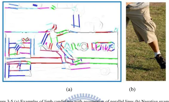
Figure 3-5 (a) Examples of limb candidates with assumption of parallel lines (b) Negative example... 24

Figure 3-6 Masks for limb patch detection ... 24

Figure 3-7 Example of clear boundary on both sides of limbs ... 25

Figure 3-8 Example of detection results of limb patches ... 25

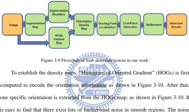
Figure 3-9 Flowchart of limb detection system in our work ... 26

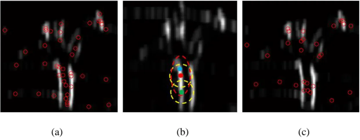
Figure 3-10 Illustration for production of orientation density map ... 27 Figure 3-11 Produce starting points for limb detection. (a) Distribution of starting

points without modification. (b) Illustration of modification. (c) Distribution of

starting points with modification. ... 28

Figure 3-12 Illustration of patch based limb detection. (a) Starting patch detection. (b) Detection of rest patches on the same limb. ... 29

Figure 3-13 Illustration of non-maximum suppression. ... 30

Figure 3-14 Refinement step in flowchart of limb detection sub-system. ... 31

Figure 3-15 Examples of head-torso training data. ... 32

Figure 3-16 Detectors of head-torso in 10 directions. ... 32

Figure 3-17 Illustration of “Image (Feature) Pyramid” and “Sliding Window Searching Scheme”. ... 34

Figure 3-18 Bounding box of torso is in green color, while searching region for head-torso is in red. ... 34

Figure 3-19 Extra step for cutting limb regions from segments. ... 35

Figure 3-20 Several results of head-torso detection are provided. ... 35

Figure 3-21 Several detection results of face detectors. Different colors denote different orientations. ... 36

Figure 3-22 Detection results of body parts. Yellow color is for face candidates. Red lines are for limb candidates. Other colors denote head-torso candidate oriented in different directions. ... 37

Figure 3-23 Illustration of the ownership of a specific face candidate for each segment. ... 38

Figure 3-24 Illustration of combination types between limb and torso. ... 39

Figure 3-25 Illustration of multi-path problem ... 39

Figure 3-26 An example of cost evaluation. ... 40

Figure 3-27 Illustration of estimation of combination direction. ... 40

Figure 3-28 Decision of joints by detection result of head-torso. (a) Joints relative to root bounding box annotated by human (b) Joints decided by position of part filters. ... 42

Figure 3-29 Estimation of width and length on silhouette of torso to adjust the positions of joints estimated from head-torso filters, which are joints in blue color. And the modified results are shown in yellow color. ... 43

Figure 3-30 Examples of limb candidates with unreasonable length to width ratio. ... 46

Figure 3-31 Two examples of mapping relations from aspect ratio to probability. ... 46

Figure 3-32 Examples of ratio between length of limb candidate and size of torso. ... 47

Figure 3-33 Two examples of mapping relations from ratio between limb length and size of torso to probability. ... 47

Figure 3-34 (a) Examples of unreasonable widths. (b) Curve for mapping relation from ratio between width of limb candidate and torso size to probability. ... 48

Figure 3-35 Illustration of evaluation for virtual limb on silhouette. ... 50

Figure 3-36 Illustration of compensation on variance from estimation of shoulder joints by cover rate. ... 50

Figure 3-37 Illustration of evaluation of overall covering rate. ... 52

Figure 3-38 Example of hip joints far from each other. ... 53

Figure 4-1 Histogram of score rank of best fit configuration. ... 55

Figure 4-2 Illustration of performance enhancement by consideration of face and limb. ... 56

Figure 4-3 Several experimental results with clear background. ... 57

Figure 4-4 Several experimental results with complex background. ... 58

List of Tables

Table 3-1 Parameters for sigmoid function used in Equation 3.20 ... 45 Table 3-2 Parameters for sigmoid function used in Equation 3.21 ... 47 Table 4-1 Recall rates of body parts ... 54

Chapter 1 Introduction

Human detection has been an active topic in computer vision for well over 15 years. The reason is the abundance of applications that can benefit from such technology. Examples include pedestrian detection for automotive safety, surveillance system for indoor care or crime alerts, and human computer interface…etc. However, up to now, there still exists no approach that can produce satisfactory results in general, with unconstrained settings while dealing with all of the following challenges: (1) illumination condition, (2) cluttered background, (3) occlusion, (4) view-point variation, (5) variable visual appearance, and (6) pose variation from a number of movable joints. In all of the six challenges, pose variation combined with view-point variation, which leads to no fixed shape of human body, is the main bottleneck. Hence, in this thesis, these two problems will be the main focus.

Before presenting our proposed method, we first briefly introduce the background of human detection and discuss the dilemma for some recent representative works. Human detection scheme can be classified into three kinds of approaches: top-down approach, bottom-up approach and hybrid approach. Tow-down approaches use global models of the human body to detect humans by minimizing a given model to image criteria. Representative works include D.M. Gavrila et. al. [2] and Felzenszwalb et al. [1]…etc. D.M. Gavrila et. al. [2] adopt a silhouette matching approach to detect pedestrian, while Felzenszwalb et al. [1] using “Deformable Part Model” leaned by latent SVM training scheme to model the human

body. Bottom-up approaches can be separated into two stages: bottom-up detection of parts and top-down procedure to obtain the best assembly. Representative works contain Alex Yong-Sang et al. [3] and Bourdev et al. [4]...etc. Alex Yong-Sang et al. [3] use the combination of lines and ellipses to describe body parts, while Bourdev et. al.

[4] cluster body parts collected from training data into group, which are similar in appearance and spatial condition, and name those groups as “Poselet”. Both works have constraints on the definition of parts, which should contain enough spatial information for inferring the positions of body center or other parts. In summary, although these works provide state-of-the-art performance, in consideration of the challenge we focused on, which is appearance variation introduced by the change of pose and view-point, we will find that all the works mentioned above will come into the same dilemma. That is the number of demanded detectors will increase exponentially in order to deal with more body poses. What’s more, if this way combined with the most popular searching scheme, exhaustive search, the computation cost will be un-acceptable.

To avoid falling into the dilemma mentioned above, we adopt the bottom-up detection scheme and constrain the targets for detection to fulfill a specific criterion, which is that targets should have high probability to be found in arbitrary pose and view-point. In Figure 1-1, we can easily find the best set of targets will be head, torso, arms and legs, which are the body parts in anatomical sense. Similar parts’ definition had been adopted for human recognition in Huttenlocher et al. [5] and had been extended for human detection and pose estimation in many works, such as [6-9].

Figure 1-1 Human in arbitrary poses

In [6], Greg Mori et al. partition a given image into small segments and make several assumptions. They assume the half limb will be well-segmented and the shape

of torso will approximate a rectangle. Finally, they search the best assembly with a greedy method. In [7] and [8], the authors assume the limbs to consist of strait lines and also assume torso is in rectangular shape. For assembly, one adopts “Integer Quadratic Programing”, while another generate “Topological Human Body Model”, inspired by “Shock Graphs”, to evaluate the combination. In [9], the authors describe the body parts by “Shape Context Descriptor” and use the “Pictorial Structural Model” to infer the assembly.

In this thesis, compared with the aforementioned works [6-9], we model limb as a combination of patches to release the strong constraints from the well-segmented and strait line assumptions. Instead of assuming the torso shape as rectangular, we describe the torso with the “Deformable Part Model” proposed by Felzenszwalb et al. [1] to allow larger variation on torso shape. In the assemble step, since our problem is human detection but not pose estimation, instead of fitting the whole model to the image with a “Pictorial Structure Model”, we only focus on the role assignment of detected parts and remove the false alarms by a greedy method. What’s more, to prevent the use of the exhaustive search, segmentation information and natural property of limbs will be used.

This thesis is organized as follows. Detail information of related works will be provided in Chapter 2. In Chapter 3, the proposed algorithm will be discussed step by step. After that, experimental results will be given in Chapter 4. Finally, some conclusion and future work will be mentioned in Chapter 5.

Chapter 2 Backgrounds

Human detection has been an active topic for a long time, and many algorithms have been proposed. In this chapter, some related works for human detection will be introduced. These algorithms can be roughly classified into two types; top-down and bottom-up, depending on the detection scheme adopted. The tow-down detection scheme uses global models of the human body to detect humans by minimizing a given model to image criteria, while the bottom-up detection scheme consists of two steps, bottom-up detection of parts and top-down inference of the best body configuration. In Section 2.1, several representative works in the top-down detection scheme will be mentioned. In Section 2.2, works in the bottom-up scheme will be presented.

2.1 Human Detection in Top-down Detection Scheme

In [2] and [10], D.M. Gavrila et al. provide an algorithm, which describes the pedestrian with global silhouette, named as templates, and establishes a template tree as shown in Figure 2-1 to represent and match variety of shape exemplars efficiently. The similarity between an image and exemplars is evaluated by the “Distance Transform” matching method as shown in Figure 2-1. Finally, the author adopts Bayesian model to set the matching threshold for each node to allow the unpromising paths in the tree traversal process eliminated early on.

(a) (b)

In [11], Dalal and Triggs first propose the famous descriptor, “histograms of oriented gradients” (HOGs), to describe the global shape of human body. The main idea is that the local appearance and shape of target object can be well characterized by the distribution of intensity gradients, which include orientations and magnitudes. The descriptors are based on evaluating well-normalized local histograms of image gradient orientations in a dense grid. An illustration of HOGs is provided in Figure 2-2. The gradients are first calculated by using difference filters, such as “Sobel Filter”. Next, these gradients are quantized and accumulated into discrete orientation bins of four cells, which equal to one block. After that, normalization will be applied on this block to handle the local variations in illumination and foreground-background contrast. A real example is provided in Figure 2-2, where the left image is a training image or testing image. We partition the image into cells and calculated the HOGs for all the cells as shown in right image. After that, we concatenate all the HOGs of each cell into a single vector, which will be the feature vector used to describe the global shape of human body. Collecting lots of positive and negative training images, we compute the feature vectors and then pass them into the “linear-SVM” training scheme proposed in [12]. Finally, the human detector will be obtained. Overview of the system is shown in Figure 2-3.

Figure 2-3 Overview of algorithm provided by Dala et al. [11]

Single rigid template or detector is not expressive enough to describe the object with highly articulated deformation, such as human body. Hence, in [1], Felzenszwalb et al. propose a “deformable part model” to handle the deformation of human body. From left to right, the model consists of root filter, part filter and deformation cost as shown in Figure 2-4. In Figure 2-4, a real detection result is provided. The frames of root filters are shown in red, while the frames of part filters which capture the deformation are shown in blue.

(a) (b)

Figure 2-4 (a) Deformable Part Model (DPM) (b) Detection results of DPM [1]

In Figure 2-5, the whole detection process is illustrated. We can find that the resolutions used to detect root filter and part filter are different in the feature pyramid. This implies that the root filter will roughly cover the entire object while the part filters will capture details in finer resolution. An example is clear shown in Figure 2-6. Face detection can be taken to demonstrate the idea clearly, where the root filter captures the face boundary in a coarse-resolution but the part filters detect the details

on face, such as eyes, nose and mouth.

Figure 2-5 Overview of algorithm provided by Felzenszwalb et al. [1]

Although the deformations of objects are captured by the movable parts, there exists anchor for each part filter. These anchors are the positions where the penalties are lowest for the part filters. These positions are latent variables, which are obtained in the training step by the “MI-SVM”, or named as “latent-SVM” here, training scheme provided in [14]. A real example is shown as the third image in Figure 2-4. As the part filter is away from the anchor position, the higher penalty will be assigned. Equation definition can be seen as the second term of the following equation:

score(𝑝₀, … , 𝑝_𝑛) = ∑ 𝐹_𝑖′ 𝑛 𝑖=0 ∙ 𝜙(𝐻, 𝑝_𝑖) − ∑ 𝑑_𝑖 𝑛 𝑖=1 ∙ (𝑑𝑥_𝑖, 𝑑𝑦_𝑖, 𝑑𝑥_𝑖2_{, 𝑑𝑦} 𝑖2), (2.1-1) where (𝑑𝑥_𝑖, 𝑑𝑦_𝑖) = (𝑥_𝑖, 𝑦_𝑖) − (2(𝑥₀, 𝑦₀) + 𝑣_𝑖). (2.1-2) are denoted as the distance between the anchor and the current position for i-th part. Besides, in this equation, 𝑝𝑖 = (𝑥𝑖, 𝑦𝑖, 𝑙𝑖) specifies the top-left corner position of the

filter at (𝑥_𝑖, 𝑦_𝑖) in the 𝑙_𝑖-𝑡ℎ level of the feature pyramid H, and 𝑝₀ means the location of the root filter. “𝑣𝑖” is a two dimensional vector specifying the position of

the anchor for the i-th part filter relative to the position of the root filter. Moreover, “𝑑𝑖” is a four dimensional vector specifying the coefficients of a quadratic function,

which defines the deformation cost for each possible displacement from the position of the part to the position of the anchor. For example, if 𝑑𝑖 = (0,0,1,1), then the

deformation cost for the i-th part is defined as the squared distance between the current position of the part filter to the position of the anchor.

In Equation 2.1, the overall score is defined as summation of detection scores from the root filter and the part filters, plus the deformation cost. “𝐹_𝑖′_{“ represents the}

coefficients of the i-th part filter. “𝜙(𝐻, 𝑝_𝑖)” means the feature vector with the top-left corner location at 𝑝𝑖. The detection score for the i-th part is defined as 𝐹𝑖′∙ 𝜙(𝐻, 𝑝𝑖).

Hence, we will find the instance with the highest score, which means the best choice of part filter locations.

2.2 Human Detection in Bottom-up Detection Scheme

In [4] and [15], Bourdev et al. introduced a new notion of parts as “poselets”, in which the key idea is to define parts that are tightly clustered both in the configuration space and the appearance space, as shown in Figure 2-7. The poselets are produced by a search procedure. A patch is randomly chosen in the image of a randomly picked person as a seed of poselet, and other examples are found by searching in images of other people for a patch where the configuration of key-points, such as shoulders or hips, is similar to that in the seed. After that, the HOGs feature will be computed for each of associated image patches. They are used as positive examples for training a linear support vector machine. At test time, a multi-scale sliding window is used to find strong activations of the poselet filters. Note that these poselets must have strong spatial information to estimate the possible locations of key-points which provides the ability to compute mutual consistency between activations. With these mutual consistencies, we can cluster the activations and produce the hypotheses of humans.

Figure 2-7 Examples of Poselets [4]

introduced. As shown in Figure 2-8, detection results of different poselet detectors are shown in different colors, and the size of the blobs means the detection scores. Mutual consistency is to calculate how close the locations of key-points are estimated by two different activations. This information is used to re-score the activations. Activation with more supporting member agreeing with the estimated key-points will lead to a higher score, while the activation not in this case will be damped. This is shown in Figure 2-8. In Figure 2-8, the authors use a saliency based agglomerative clustering with pairwise distances based on consistency of the empirical key-point distributions predicted by each poselet. Finally, the bounding boxes and segmentations are predicted by the poselets in each cluster as shown in Figure 2-8.

Figure 2-8 Illustration of algorithm provided by Bourdev et al. [15] (a) Detection results of Poselet in different color, called activations (b) Illustration of Mutual Consistency (c) Saliency based clustering in

greedy manner (d) Detection and segmentation results.

by the combination of shape-tokens, which consist of several line segments and ellipses. An overview of this contour based recognition method is provided in Figure 2-9. In the first step, lots of shape-tokens will be extracted from training set, and then clustered into different code-words of the codebook. Next, a discriminative sub-set of codebook will be extracted. Instead of cluster size, the extraction is based on the score calculated from shape and geometric qualities and a radial ranking will be applied. Note that for each shape-token, the relative position of object center will be recorded. Hence, the final positions of objects will be decided by a voting scheme. Besides, the bounding boxes will be determined based on the shape-tokens used.

Figure 2-9 Overview of algorithm provided by Alex Yong-Sang Chia et al. [3]

Up to now, the definitions of parts used for detection are learned from training data and these parts need to contain strong spatial information in order to infer the locations of key-points on body configuration or the center of target object. The following references in [6-9] adopt different ways. They directly define the parts for detection in the natomical sense, which means that the parts will be head, torso, forearm, upper-arm, thigh or shank. These references are closely related to our work in this thesis.

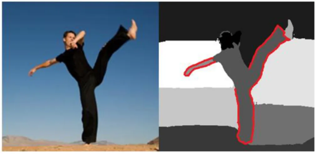
the body parts, such as limb, torso and head, based on information of segments. For limb, the author assumes the half limbs, such as forearm, upper-arm, thigh or shank, will be well segmented, which means the half limb will be represented by single segments. In order to detect half limbs, lots of hand-segmented half limbs are extracted for training. Several examples are shown in Figure 2-10. Features used to describe the half limb are contour, shape, shading and focus. Sigmoid function is used to transform the feature value into a probability-like quantity. These values will be combined linearly and the weights will be learned from training data with a linear regression training scheme. Finally, the number of candidates to be extracted can be seen as the threshold for half limb detection.

For torso, the shape is assumed to be rectangular, and may consist of more than one segment. The features used are the same as the features used for half limb only without shading. The training of weights for feature combination is totally the same. For inference of configuration, we need to know the orientation of torso and the locations of body joints. Hence, for each torso candidate and each orientation, the best matching head will be decided. A candidate head may consist of one or two segments. The same set of cues, contour, shape and focus are used to evaluate the score of a candidate head. The combination score of head and torso consists of the score of head and the score of torso, plus the simple score to describe the relative positions. Finally, we sort the possible combination of head and torso by their score and choose a finite number of combinations as candidates for the inference of configuration. Several examples are shown in Figure 2-10.

(a) (b)

Figure 2-10 (a) Examples of human-segmented half limbs for training, (b) Torso candidates are provided by combination of segments. [6]

As having the part candidates and information of joints, the next step is the inference of configuration. The method adopted by the author is the exhaustive search. For each torso candidate, the best limb will be independently selected for each joint. The number of possible configurations is evaluated as (𝐿₃) ∙ 8 ∙ 7 ∙ 6 ∙ 23∙ 𝑇 . L means the number of half limb candidate, which is usually around 5~7, and T means the number of head-torso candidates, which is set to be 50. Here, the author assumes that for each configure, at least three half limbs can be found. Besides, there are 8 kinds of role for each half limb candidate. Hence, the number of possible combination of three half limbs will be 8 ∙ 7 ∙ 6. However, the polarity of half limbs is also considered. Hence, a multiplication of 23 will be needed. This exhaustive search will lead to 2-3 million partial configurations. A “Constraint Satisfaction” strategy will be used to suppress physically impossible configures. The constraints used are relative widths, length given torso, adjacency and symmetry in clothing. With this strategy, the number of left configures will be approximately 1000. Finally, these configures will be sorted by the total scores, which are the linear combination of scores of limbs and head-torso. Several examples are shown in Figure 2-11.

Figure 2-11 Several detection results of [6]

In [7], the author first preprocesses the image by using the “local Pb operator” to compute the soft edge map. After that, “Canny’s hysteresis” is used to convert the soft edge map into contours, which are recursively split into piecewise straight lines. Finally, “constrained delaunay triangulation” (CDT) is applied to transform the scale-invariant discrete line structure into a set of triangles.

As the triangulation map is ready, the candidates of limb and torso will be extracted with the assumption of being a combination of parallel lines. Constraint for torso is oriented upward. With body parts, the configuration inference can be seen as a label assignment problem, which means the decision of the role for each part candidate in the configuration. The best configuration will be inferred by the discussion of simple unary constraints and pairwise constraints, which are aspect ratio, low-level score, scale consistency, appearance consistency, orientation consistency and connectivity. These constraints will be modeled by Gaussian distributions. The inference problem can be modeled as the minimization of the following equation:

∑ ∑ 𝑓_𝑘′_(𝑙 1, 𝜋(𝑙1), 𝑙2, 𝜋(𝑙2)) 𝑘 + ∑ 𝑑(𝜋(𝑙)), 𝑙 𝑙1,𝑙2 (2.3-1) where 𝑓_𝑘′₌ (𝑓𝑘−𝜇𝑘)2 𝜎_𝑘2 . (2.3-2)

body label. 𝜋(𝑙_𝑖) represents the part candidate which is assigned with 𝑙_𝑖 body label. Besides, 𝑑(𝜋(𝑙)) is used to measure the quality of an individual part candidate. Minimizing Equation 2.3 can be further written as an integer quadratic programming problem (IQP), which is expressed as follows:

min 𝑄(𝑥) = 𝑥′_{𝐻𝑥 + 𝑑}′_{𝑥 𝑠𝑢𝑏𝑗𝑒𝑐𝑡 𝑡𝑜 𝐴𝑥 = 𝑏, 𝑥 ∈ {0,1}}𝑛_{, (2.4-1)}

where

H(i, j) = ∑ 𝑓_𝑘′_{(𝑙(𝑖), 𝑝(𝑖), 𝑙(𝑗), 𝑝(𝑗)).} 𝑘

(2.4-2)

Directly optimize Equation 2.4 is an NP hard problem. An approximation is deducted which is a linear bounding function allowing efficient inference as shown in the following equation: min L(x) = ∑ (𝑞_{𝑖 𝑖}+ 𝑐_𝑖)𝑥_𝑖 L(x) < 𝑄(𝑥) 𝑓𝑜𝑟 𝑎𝑙𝑙 𝑥, _(2.5-1) where 𝑞_𝑖 = 𝑚𝑖𝑛_𝑥∑ 𝐻(𝑖, 𝑗)𝑥_𝑗 𝑗 . (2.5-2)

Finally, the greedy search is adopted. We fix one candidate for specific label and find the best assignment for other candidates. We repeat the procedure to find the configuration with minimum constraint cost. An example for illustration of the overall system is provided in Figure 2-12.

(a) (b) (c) (d) (e) (f)

Figure 2-12 Illustration of algorithm provided in [7] (a) Input image (b) Edge map (c) Result of Constrained Delaunay Triangulation (d) Part candidates in parallel lines with same color (e)

Configuration found by Integer Quadratic Programming (f) Approximate Segmentation

directly as shown in [7], the authors relax the constraint so that they need only one straight line segment to handle the missing segment caused by cluttering, occlusion or shape variation. As one straight line is extracted, the “Distance Transform (DT)” matching provided in [10] will be applied. The matching score between parallel line templates in different sizes and orientations and the distance transform of edge map obtained by “Canny Edge Detector” will be evaluated at every possible position. The formula form is provided as follows:

𝐷𝑇_𝑇𝑙 = 1

|𝑇_𝑙|∑ 𝐼𝐸′(𝑡) 𝑡∈𝑇𝑙

, _(2.6)

where 𝑇_𝑙 represents the prior shape of limb, which is parallel lines. |𝑇_𝑙| denotes the number of edge points in 𝑇_𝑙. 𝐼_𝐸′ means the DT of binary edge map 𝐼_𝐸. The templates used for torso is the same as the templates for limb. The scale of torso will be inferred from the scale of limbs based on the anthropometric data provided in [16]. For head, the template shape is a circle.

With part candidates, the best body configuration is inferred by the lowest value of dissimilarity 𝐷_𝐻 as expressed in the following equation:

𝐷_𝐻 = 𝑤_𝑔𝐷_𝑔+ 𝑤_𝑡𝐷_𝑡𝑜𝑝+ 𝑤_𝑎𝐷_𝑎𝑝𝑝+ 𝑤_𝑙𝐷_𝑙𝑔. (2.7) In Equation 2.7, {𝑤} means weights which are learned from training data. 𝐷_𝑔 is a

term dedicated to pruning configurations that are not physically valid. 𝐷𝑡𝑜𝑝

corresponds to a topological matching between the part assembly and a model of the human skeleton. This model is inspired by the “shock graphs” mentioned in [17]. 𝐷_𝑎𝑝𝑝 encodes prior information about the symmetry in clothing and support these

assemblies for which the appearance of left and right limbs is similar. The last term 𝐷_𝑙𝑔 corresponds to a more global reasoning about the configuration, which is

dedicated to estimating a combined image likelihood of the assembly by explicitly taking into account self-occlusion.

A brief illustration of the system flow is shown in Figure 2-13.

Figure 2-13 Illustration of algorithm provided in [8].

In [9], the authors claim that the performance of detection is highly dependent on the discriminative part classifiers. Hence, in this work, densely sampled “shape context descriptor” provided in [18] is adopted to describe body parts. Moreover, the Adaboost training scheme proposed by [19] is applied. Finally, with part candidates, the inference of configure follows the same steps as proposed in [5] with the usage of “Pictorial Structural Model”. The equation form of this model is provided as follows:

p(L|D) ∝ 𝑝(𝑙₀) ∙ ∏ 𝑝(𝑑_𝑖|𝑙_𝑖) 𝑁 𝑖=0 ∙ ∏ 𝑝(𝑙_𝑖|𝑙_𝑗) (𝑖,𝑗)∈𝐸 . (2.8)

In this equation, p(L|D) means that given the image feature, D, what will the probability of configuration L be. This probability will be proportional to the multiplication of three terms shown in the right portion of Equation 2.8. 𝑝(𝑙₀) denotes the probability for the location of torso to be at 𝑙₀. ∏𝑁_𝑖=0𝑝(𝑑_𝑖|𝑙_𝑖) represents the probability for the rest part to be placed at 𝑙_𝑖. 𝑑_𝑖 means the evidence map for the the i-th part. Finally, ∏_{(𝑖,𝑗)∈𝐸}𝑝(𝑙_𝑖|𝑙_𝑗) denotes the spatial relation between the position of the i-th part and the position of the j-th part. One thing needs to be

mentioned is that torso candidates will be detected first in this work. Several results of this work are provided in Figure 2-14.

Chapter 3 Proposed Method

Recall the goal of our work is to provide a human detection method to handle the intra-class variation caused by the change of poses and view-points as much as possible. In order to prevent the demand of lots of detectors to cover the intra-class variation, bottom-up scheme and constrained body parts defined in anatomical sense are going to be used. One thing needs to be mentioned is that, instead of considering head and torso separately, we detect them at the same time in order to avoid the high false alarm rate introduced by each of them alone. Moreover, the face information will be extracted to support the identification of head-torso candidates.

In the adopted bottom-up scheme, our system can be divided into two portions, information collection and information integration, as the last two steps in Figure 3-1. Information collection is the step of detecting parts. Information integration is the step to integrate the detection results; that is, to decide which parts should belong to the same person and what are these parts: face, head- torso, arm, leg or false alarm from background.

In the information collection step, despite of the existence of constraint on the definition of parts for detection, the computation cost is still high due to the exhaustive search on the scale, position and orientation of parts. Hence, an extra step to reduce the searching space is introduced. Here, we will first partition the image into segments to create a discrete searching space.

Hence, our system consists of three portions: image decomposition, collection of information and information integration, as shown in Figure 3-1. In Section 3.1, image decomposition will be discussed. After that, the method of detection for limbs, faces and head-torsos will be mentioned in Section 3.2. Finally, in Section 3.3, the way to deal with information integration will be provided.

Figure 3-1 Flowchart of our algorithm

3.1 Image Decomposition

As aforementioned, we will partition the image into segments and use the region information to reduce the searching space, with the assumption that it is rare to have body parts existing within smooth regions.

Segmentation can be regarded as a pixel clustering problem. There are lots of clustering algorithms in the literature and these algorithms can be classified into four kinds of methods: “partition-based methods”, “hierarchical clustering methods”, “probabilistic model-based clustering methods” and “spectral clustering methods”.

Here, the proposed method belongs to “spectral clustering methods”.

“Spectral clustering methods” are graph partition based methods. Hence, the first

thing is to establish the graph. Here, image pixels are defined to be nodes in the graph. The definition of edges is called affinity matrix. Each element in the affinity matrix represents the relation between two pixels or two nodes. There are three kinds of methods for the definition of affinity matrix which are “K-nearest Neighbors”, “Radius Based Method” and “Gaussian Model Based Method”. As a graph is obtained,

we can write the cost function as shown in the following equation: min ∑ 𝐴_𝑖,𝑗

𝑖,𝑗

∙ (𝛼_𝑖− 𝛼_𝑗)2, _(3.1)

where i, j are indexes of nodes in the graph or indexes of pixels in the image. 𝐴𝑖,𝑗

denotes the affinity relation between 𝑛𝑜𝑑𝑒_𝑖 and 𝑛𝑜𝑑𝑒_𝑗. 𝛼_𝑖 & 𝛼_𝑗 are cluster labels for 𝑛𝑜𝑑𝑒𝑖 and 𝑛𝑜𝑑𝑒𝑗. With this equation, our goal will be to find the optimal cluster

follows:

min 𝛼𝑇_{∙ 𝐿 ∙ 𝛼, (3.2)}

where L = D − A is called as “Graph Laplacian Matrix”. D = ∑𝑁_𝑗=1𝐴(𝑖, 𝑗) is the degree matrix of graph. A denotes the affinity matrix of graph and N is the number of nodes. Finally, 𝛼 represents the matrix of cluster labels for all nodes. Here, the definition of the affinity matrix, A, is adopted from the representative work, spectral matting, proposed by Levin et al. in [20]. Note that instead of global affinity calculation, only local affinity will be calculated. This means that we only consider the affinities among pixels in a local region. For a local region as 𝜔_𝑞, the definition of A is provided in the following equation:

A = ∑ 𝐴_𝑞 𝑞 , (3.3-1) where 𝐴𝑞(𝑖, 𝑗) = { 1 |𝜔𝑞| (1 + (𝐼𝑖− 𝜇𝑞) 𝑇 ∙ (Σ𝑞+ 𝜀 |𝜔𝑞| 𝑈) −1 ∙ (𝐼𝑗− 𝜇𝑞)) (𝑖, 𝑗) ∈ 𝜔𝑞 0 𝑜𝑡ℎ𝑒𝑟𝑤𝑖𝑠𝑒. (3.3-2)

In Equation 3.3, 𝐼𝑖 and 𝐼𝑗 denote the colors of the i-th and the j-th pixels in input

image 𝐼. 𝜇_𝑞 is the 3x1 mean color vector of image in the region, 𝜔_𝑞. Σ_𝑞 is the covariance matrix in the same region. Finally, |𝜔_𝑞| means the number of pixels in the region and 𝑈 represents the 3x3 identity matrix. Note that the graph Laplacian matrix is also called matting Laplacian in [20].

The general method to solve Equation 3.2 is to find the eigenvectors of the matting Laplacian and sort these eigenvectors based on the eigenvalues in ascending order. After that, they map data points into the space constructed by eigenvectors. Finally, K-means method is applied to classified data points into clusters.

One thing needs to be noticed is that the computation complexityfor obtaining eigenvectors is O(𝑁3), where 𝑁 denotes the number of pixels in [20]. This leads to

slow speed when handling large images. Hence, instead of taking each pixel as a node, we group pixels into cells and decompose the cell-based matting Laplacian, 𝐿_𝑐. The equation for 𝐿_𝑐 is provided as follows:

𝐿_𝑐 = 𝑚̅𝑇_{∙ 𝐿 ∙ 𝑚̅, (3.4)}

where 𝑚 is the mapping of pixels into cells. 𝑚̅ denotes the mapping relation normalized by the number of pixels in each cell. Finally, two different segmentation results are provided in Figure 3-2 and Figure 3-3, respectively.

Figure 3-2 Result of segmentation. Different color means different segment.

3.2 Information Collection

In this section, information collection will be presented as detection of body parts. The body parts to be detected can be separated into three types, which are limbs, head-torso and face. Method for detection of limbs will be discussed in Section 3.2.1. After that, the adopted algorithm for detection of head-torso and face will subsequently be mentioned in Sub-section 3.2.2 and 3.2.3.

3.2.1 Detection of Limb

In this sub-section, the implementation for limb detection and the reason for this implementation will be described in detail. Firstly, we will review the methods for limb detection adopted in [6-9] and describe the limitations of these works. After that, the ideas to overcome the limitations will be provided. Finally, the implementation detail will be described step by step.

Go back to the related works. In [6], the authors assume the half limb, which means forearm, upper-arm, thigh or shank, will be well segmented as shown in Figure 3-4. This assumption will fail in the case shown in Figure 3-4.

(a) (b)

Figure 3-4 (a) Example of well-segmented half limb [6] (b) Failure of well-segmented approach.

In [7-8], limbs are assumed as the combination of parallel lines or at least one side of limb can be detected as a straight line as shown in Figure 3-5. This assumption cannot handle the shape variation as shown in Figure 3-5. In [9], the shape context

descriptor is used to describe body parts. However, for simple shapes, such as limbs only, shape context is too complicated for description and may introduce high computation cost.

(a) (b)

Figure 3-5 (a) Examples of limb candidates with assumption of parallel lines (b) Negative example

In order to prevent these limitations, we describe each limb as a combination of patches, which are simple masks with nine different orientations as shown in Figure 3-6. With this description, limbs will be detected by exhaustive search. In this way, instead of using the restriction of well segmented limbs, we only need the limbs to have clear boundary on both sides and we allow arbitrary connections on the ends of limbs, as shown in Figure 3-7. Moreover, the variation of limb shape shown in Figure 3-5 can be handled by the displacement and scale change of patches. One example is provided in Figure 3-8.

Figure 3-7 Example of clear boundary on both sides of limbs

Figure 3-8 Example of detection results of limb patches

Up to now, we have the descriptor for limbs and use a detection scheme with exhaustive search. Exhaustive search for all the positions, orientations and scales is quite inefficient. Hence, instead of exhaustive search, we’d like to find some other information to reduce the searching space. The information used here will be segmentation boundary from the previous image decomposition step and the natural characteristic of limbs: limbs often appear at regions with high density of isotropic orientation. In order to use the information, we make two assumptions: (1) the boundary of limbs will be included in the boundary of segmentation, and (2) the

density of isotropic orientation of limbs will be relatively high in the local region. Based on these assumptions, density maps for each orientation can be established. With density maps, we can sample a few initial points and apply the exhaustive search method for the positions and scales in local region.

In the following, we will follow the order of the block diagram as shown in Figure 3-9 to describe the limb detection step by step.

Figure 3-9 Flowchart of limb detection system in our work

To establish the density maps, “Histogram of Oriented Gradient” (HOGs) is first computed to encode the orientation information as shown in Figure 3-10. After that, one specific orientation is extracted from the HOGs map, as shown in Figure 3-10. It is easy to find that there exist lots of background noise in smooth regions. The noise leads to lots of meaningless initial points and increase the computation cost. In order to retain meaningful information and filter out noise, a morphological method is applied on the segmentation map. The segmentation boundary map is then extracted out as shown in Figure 3-10. We use this segmentation boundary map to retain the useful orientation information and an example of the filtered result is shown in Figure 3-10. Finally, Gaussian smooth filter is convolved with the filtered orientation map, and the density map for specific orientation will be obtained as shown in Figure 3-10. We repeat all the steps until all the density maps in different orientations are produced.

Figure 3-10 Illustration for production of orientation density map

Up to now, the density maps for all orientations are obtained. The next step is the extraction of discrete points as the initial points. The algorithm used here is the “mean-shift” algorithm and the features are position and density value. After all the

points are clustered, the position of the center for each cluster will be taken as the position of the initial point. However, there are two problems for the direct usage of the original “mean-shift” algorithm. One is the slow speed and another is unreasonable distribution of clusters.

density map till convergence. To solve this problem, we can approximate the result by assigning all the points only one time. Firstly, we sort all the points on the density map in the descent order. After that, one point is taken and the distances to the centers of the established clusters are computed for each iteration. If no cluster exists or all the distances are larger than the clusters’ radii, we establish a new cluster for the current point. We repeat the steps until all points are assigned.

The second problem can be seen in Figure 3-11. There are too many points spreading along the orientation which means that there are too many initial points for a single limb candidate. To avoid the waste of computation, a modified distance equation is provided as follows:

dist = 𝑤1× 𝑜𝑟𝑖 + 𝑤2× 𝑜𝑟𝑡ℎ𝑜𝑟𝑖+ 𝑤3× 𝑑𝑣 , 𝑤1 = 𝑤2 > 𝑤3, (3.5)

where 𝑜𝑟𝑖 means orientation, 𝑜𝑟𝑡ℎ_𝑜𝑟𝑖 means orthogonal orientation, and d_v denotes density value. In Equation 3.5, smaller weights are provided along the orientation which means a larger radius is used along this direction. The difference can be seen in Figure 3-11. The red dashed circle is the result of the modified process, and the yellow dashed circle is the result without modification.

(a) (b) (c)

Figure 3-11 Produce starting points for limb detection. (a) Distribution of starting points without modification. (b) Illustration of modification. (c) Distribution of starting points with modification.

positions and scales along the orthogonal orientation, as shown in Figure 3-12. Once a patch is detected, as shown in Figure 3-12 with the bright green bounding box, its estimated scale and position will be used as prior information to detect the remaining patches on the same limb, as shown in Figure 3-12 with the red bounding boxes. With this detection scheme, we can reduce the searching space dramatically.

The last step in limb detection is refinement. This step can be divided into three portions: non-maximum suppression, connection of fragments on the same segment and connection of fragments on different segments.

(a) (b)

Figure 3-12 Illustration of patch based limb detection. (a) Starting patch detection. (b) Detection of rest patches on the same limb.

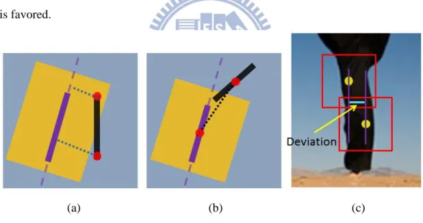
Firstly, as mentioned previously, more than one initial point may be adopted for a single limb, as shown in Figure 3-11. Hence, a “non-maximum suppression” algorithm is implemented. One thing needs to be mentioned is that we only consider the suppression for limb candidates on the same segment. An illustration of the algorithm is provided in Figure 3-13. Linear equation for one of limb candidates, called a basic candidate, is firstly generated. After that, we calculate the shortest distances from the end-points of another candidate, as shown in Figure 3-13. The summation of distances is compared to the width of the basic candidate. Moreover, we

check the distance between centers of limb candidates to prevent the case of suppression shown in Figure 3-13. If both the distance summation of end-points to line of basic candidate is less than the width of basic candidate and the distance between centers is less than a half length of the basic candidate, we further compare the scores of limb candidates. We choose the larger one and suppress the other. The score used here is composed of four ingredients: width, length, degree of deviation and the average detection score from patches as member of limbs. Here, limb candidate with a larger width and longer length will be favored. The degree of deviation is defined as the average of deviations collected from the displacements between neighboring patches along the orthogonal orientation, as illustrated in Figure 3-13. Due to the rigidness of half limb, the limb candidate with the smaller deviation is favored.

(a) (b) (c)

Figure 3-13 Illustration of non-maximum suppression.

Secondly, due to the discrete orientation angle of patch detector shown in Figure 3-6, we expect the disconnection for the patches on the same limb, as illustrated in Figure 3-14. Hence, we need to apply an extra step to connect these fragments back to a single limb. The criteria used are the width ration between fragments, the distance between end-points and the difference between orientations. The threshold for width ration is two. The threshold for distance between end-points is set to the maximum

width of fragments. Finally, the threshold for orientation difference is 20 degrees. The third portion is similar to the second portion just mentioned. It is caused by the color difference on different regions of limb. An example is shown in Figure 3-14. The connection criteria used is the same as the ones used in second portion. One thing needs to be noticed is that the fragments to be connected should fulfill one criterion. That is, over 80 percents of the segment region on which the fragment is detected should be covered by the region of fragment. This can be seen in Figure 3-14. Finally, we merge the segments which are connected together.

(a) (b) (c)

Figure 3-14 Refinement step in flowchart of limb detection sub-system.

3.2.2 Detection of Head-torso

In this sub-section, instead of detecting head and torso separately, we detect them together. The reason is that the shapes of head and torso are short of decisive information to be distinguished from background noise. Hence, in order to suppress false alarms, we consider the combination of head and torso. The following is the discussion of the adopted head-torso detection method and the targets to be detected. It can be seen in Figure 3-15 that the head-torsos are oriented in multiple directions and the shape boundaries are highly deformed due to different clothing, occlusions, foreshortening, difference from side-view and frontal view, and also the relative displacement between head and torso. Hence, a single template or detector as

provided in [11] is needed. Here, the “deformable part model” proposed by [1] is applied to capture the shape deformation by using deformable part filters. Note that the feature used in [1] is HOGs. Instead of providing 18 directions, only 10 directional training data can fulfill the demand for the training of the detector training. That’s because the training/testing scheme will automatic flipped the image along the vertical orientation to handle the head-torso in mirror-symmetric direction. Finally, detectors in different 10 directions are provided as shown in Figure 3-16.

Figure 3-15 Examples of head-torso training data.

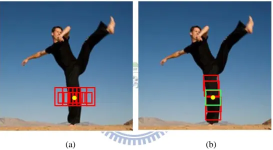
With trained detectors, the next step is the application of detectors to detecting head-torso candidates. The searching scheme used in [1] is exhaustive search, which consists of “image (feature) pyramid” plus “sliding window” as shown in second row of Figure 3-17. This searching scheme leads to high computation cost. Hence, we find extra information to reduce the searching spaces of parameters, which are positions (x, y) and scale s. In our work, we agree with the assumption used in [21] which

indicates that there exists dominant colors for torso region on human body in most cases. This assumption can be seen in Figure 3-15. With this assumption, the size of head-torso can be approximated by the size of segment. That is, we estimate the scale and position of head-torso candidates by the information of segments. In Figure 3-18, the bounding box in green denotes the region of torso, and the searching region is shown in red. Searching region will be re-scaled for fitting different scales of feature maps. The estimated scale for searching torso in feature maps for torso is provided in the following equations:

𝑠𝑐𝑎𝑙𝑒_{𝑒𝑠𝑡𝑖𝑚𝑎𝑡𝑒𝑑} = max (𝑟𝑜𝑢𝑛𝑑 (1.5 ∙ 𝑠𝑖𝑧𝑒𝑡𝑜𝑟𝑠𝑜

𝑠𝑏𝑖𝑛 ∙9₂ ) , 1), (3.6-1) 𝑠𝑐𝑎𝑙𝑒_{𝑢𝑝𝑝𝑒𝑟𝑏𝑜𝑢𝑛𝑑} = 𝑠𝑐𝑎𝑙𝑒_{𝑒𝑠𝑡𝑖𝑚𝑎𝑡𝑒𝑑}− 𝑖𝑛𝑡𝑒𝑟𝑣𝑎𝑙 − 1, and (3.6-2)

𝑠𝑐𝑎𝑙𝑒𝑙𝑜𝑤𝑒𝑟𝑏𝑜𝑢𝑛𝑑 = 𝑠𝑐𝑎𝑙𝑒𝑒𝑠𝑡𝑖𝑚𝑎𝑡𝑒𝑑+ 𝑖𝑛𝑡𝑒𝑟𝑣𝑎𝑙 + 1, (3.6-3)

where 𝑠𝑖𝑧𝑒𝑡𝑜𝑟𝑠𝑜 means the diagonal length of green bounding box as shown in

Figure 3-18. The constant 1.5 denotes the size ratio between head-torso and torso. sbin represents the size of cell used in calculation of HOGs feature pyramid. The

constant 2 means the size of cell in the first scale of HOGs feature pyramid is 𝑠𝑏𝑖𝑛₂ .

The constant 9 is the size of root filter for head-torso detection. Finally, “interval” is the scale difference between two resolutions in the HOGs feature pyramid. Extra step is required to handle the cases as shown in Figure 3-19. In these figures, the color of

legs or arms is the same with the color of torso. Hence, we need to delete the region of limbs to avoid false estimation. Finally, two detection results are provided in Figure 3-20.

Figure 3-17 Illustration of “Image (Feature) Pyramid” and “Sliding Window Searching Scheme”.

Figure 3-19 Extra step for cutting limb regions from segments.

Figure 3-20 Several results of head-torso detection are provided.

3.2.3 Detection of Face

The reason to detect face is to handle the missing cases of head-torso detection caused by serious deformation, such as foreshortening more than 40 degrees and serious occlusion…etc. Moreover, faces can be seen as extra information to support the detection of correct head-torso and the suppression of the false alarms. Both benefits are mainly from the discriminative features of faces.

The algorithm used for face detection is the famous face detector proposed in [22]. In this algorithm, Viola and Jones first propose “integral image” to accelerate the extraction of features. After that, an Ada-boost learning algorithm is applied to select a small number of critical visual features from a very large set of potential features extracted from training data. Finally, the selected critical visual features for examining the testing images are arranged in cascade form for speed-up which filters out most patches in the first few steps.

System Toolbox” on Matlab. There exists both frontal and profile face detectors. Both detectors are designed for human standing upward only. Hence, an extra step is used which rotates the image into 18 directions. Finally, to handle multiple detections on the same face, the non-maximum suppression process is applied. Several detection results are shown in Figure 3-21.

Figure 3-21 Several detection results of face detectors. Different colors denote different orientations.

3.3 Information Integration

Up to now, candidates of body parts have been detected and spread over the whole image as shown in Figure 3-22. With the adoption of a bottom-up detection scheme, the next two steps will be the combination of body parts to provide possible

configurations and the score evaluation of all configurations.

Figure 3-22 Detection results of body parts. Yellow color is for face candidates. Red lines are for limb candidates. Other colors denote head-torso candidate oriented in different directions.

For the combination step, direct exhaustive combination between part candidates will introduce lots of unreasonable configurations. To prevent this problem, an extra filtering step is adopted. With the dominating color assumption mentioned in Section 3.2.2, each segment is treated as a torso candidate. Hence, we first discuss the possibility for the combination between part candidates and the specific torso candidate. After that, only part candidates with high possibilities will be preserved as a torso candidate to establish configurations. This portion is provided in Section 3.3.1. With the knowledge of which part candidates can be used to establish the configurations for each torso candidate, we exhaustively produce all possible configurations and evaluate their scores in Section 3.3.2. Finally, with these scores, the best configuration is extracted for each torso candidate.

3.3.1 Combination Pre-filtering

In this sub-section, we will discuss which part candidate can be combined with a specific torso candidate. For the candidates of head-torso, we detect head-torso candidates for each segment separately and ask these candidates to overlap the

segment with a percentage above a specific threshold. Hence, for each segment, it could be a torso.

For the face candidates, we know the orientation difference between face and torso can’t be over 90 degrees. Hence, a half circle mask is produced to decide the ownership of face candidates, as shown in Figure 3-23. Segments covered by the red half circle mask can be combined with this face candidate.

Figure 3-23 Illustration of the ownership of a specific face candidate for each segment.

Finally, we discuss the possibilities of combinations between limb candidates and torso candidates. Firstly, we need to know the reasonable combination types between limb and torso. In our approach, there are four major types. The first one is that limbs are on the same segment as the torso candidate, as illustrated in Figure 3-24. The second one is that the limbs segments are directly connected with a torso segment. An example is also provided in Figure 3-24. The third type is that a segment exists between a limb segment and a torso segment, which can be seen in Figure 3-24. The final type is that two segments exist between a limb segment and a torso segment. A real example is shown in Figure 3-24. Note that we don’t consider the cases with more than two segments exist between limb segment and torso segment.

(a) (b)

Figure 3-24 Illustration of combination types between limb and torso.

As we know the combination types, we can model the possibility evaluation problem as a multi-path optimization problem as shown in Figure 3-25, where “T” means torso, “L” means limb and “S” means in-between segment. For each path, we evaluate the cost, which is equal to the inverse of possibility. After that, we choose the path with the lowest cost and compare the cost with a pre-defined threshold. If the cost is lower than the threshold, this limb candidate will be preserved to establish a configuration for current torso candidate.

Figure 3-25 Illustration of multi-path problem

Features used to calculate costs are the summation of the areas of in-between segments in the path and the way that the current limb combines with the first in-between segment. Examples are shown in Figure 3.26. The torso region is bounded by the red color boundary. A correct path is bounded by the blue color boundary, while an incorrect path is bounded by the green color boundary. Large areas of

in-between segments will lead to a high cost. Limbs combining with neighboring segments along similar orientations will lead to a low cost. Equations are provided as follows: Cost_{𝑝𝑎𝑡ℎ} = Penalty_{𝑡𝑦𝑝𝑒}∙𝐴𝑟𝑒𝑎𝑠𝑒𝑔𝑚𝑒𝑛𝑡 𝐴𝑟𝑒𝑎_{𝑡𝑜𝑟𝑠𝑜} , (3.15-1) where 𝑃𝑒𝑛𝑎𝑙𝑡𝑦𝑡𝑦𝑝𝑒 = S(min(r3 + r4 + r2 − r1, r3 + r4 + r1 − r2)), _(3.15-2) S(∙) = 𝑟𝑒𝑠𝑐𝑎𝑙𝑒 𝑣𝑎𝑙𝑢𝑒 𝑖𝑛𝑡𝑜 1~5, and (3.15-3)

𝐴𝑟𝑒𝑎_{𝑠𝑒𝑔𝑚𝑒𝑛𝑡} = summation of areas of middle segments. (3.15-4)

𝑃𝑒𝑛𝑎𝑙𝑡𝑦𝑡𝑦𝑝𝑒 is decided by the way that the current limb combines with the

neighboring segment. On the other hand, “r1,r2,r3,r4” are the overlapping regions between the neighboring segment and the mask used for estimating the direction of the combination. This is illustrated in Figure 3.27.

Figure 3-26 An example of cost evaluation.

3.3.2 Establishment and Score Sorting of Configurations

As we have the part candidates, which can be used as a torso candidate, the next step will be the establishment of configurations based on these part candidates. The establishment of configurations can be seen as the labeling of part candidates which is the decision of what role the specific part candidate will be. For different kinds of part candidates, there exist different choices. For each face candidate, it may be a face or a false alarm. For each head-torso candidate, it may be a head-torso or a false alarm. For each limb candidate, it may be a left/right forearm, a left/right upper-arm, a left/right shank, a left/right thigh, a left/right full-arm, a left/right full-leg or a false alarm. How do we decide the role for each part-candidate? Firstly, fixed references need to be set. The references used here are the body joints, which are center of head, shoulders and hips. With these fixed body joints, we can start to evaluate the score or possibility of each part-candidate to be a specific role.

Where do these joints come from? There are several sources. For the joint of head, it may come from the candidates of head-torso or face. For the joints of shoulders and hips, it may come from the candidates of head-torso or limb. The shoulder joints from candidates of head-torso are provided by the trade-off between two possibilities. One is the joints relative to the bounding box of the detection result, which are annotated by human and are based on the model shown in Figure 3-16. This is shown in Figure 3-28. Another one is the joints deducted from the positions of part filters of detection result as shown in Figure 3-28. The reason for this implementation is due to the unstable performance of part filters. It can be seen in Figure 3-16 that there exists no part filter to describe the shape of shoulders directly. This is because the high variance introduced by the movement of two arms. The information used for trade-off is the detection score of head-torso candidate. The trade-off equation is provided as follows: