利用球面輻射基底函數對BRDF及環境光源之重要性取樣

全文

(1)國立交通大學多媒體工程研究所碩士論文. 利用球面輻射基底函數對 BRDF 及環境光源之重要性取樣 Importance Sampling from Product of the BRDF and the Illumination using Spherical Radial Basis Functions. 研究生：江慶臻指導教授：施仁忠. 教授. 中華民國九十六年六月.

(2) 利用球面輻射基底函數對 BRDF 及環境光源之重要性取樣 Importance Sampling from Product of the BRDF and the Illumination using Spherical Radial Basis Functions. 研究生：江慶臻. Student：Qing-Zhen Jiang. 指導教授：施仁忠. Advisor：Zen-Chun Shih. 國立交通大學多媒體工程研究所碩士論文. A Thesis Submitted to Institute of Multimedia Engineering College of Computer Science National Chiao Tung University in partial Fulfillment of the Requirements for the Degree of Master in. Computer Science June 2007 Hsinchu, Taiwan, Republic of China. 中華民國九十六年六月.

(3) 利用球面輻射基底函數對 BRDF 及環境光源之重要性取樣. 研究生：江慶臻. 指導教授：施仁忠教授. 國立交通大學多媒體工程研究所. 摘. 要. 我們藉由球面輻射基底函數（SRBF）的特性，針對高動態範圍（HDR）環境光源以及經由測量所得的雙向反射分佈函數（BRDF）這兩種函數的乘積，提出一種新的重要性取樣技術。在前處理時，我們透過非線性最佳化的演算法，將高動態範圍環境光源貼圖以及雙向反射分佈函數轉換成球面輻射基底函數的表示形式。在執行顯像運算時，我們先計算出兩個球面輻射基底函數的乘積，然後根據球面輻射基底函數的表示形式，提出有效率的重要性取樣方法，其產生出來的取樣分佈可以契合球面輻射基底函數所描述的資料分佈。此方法可以在全域光源照射的環境下，有效率地繪製包含多種複雜材質以及高動態範圍環境光源的場景。. I.

(4) Importance Sampling from Product of the BRDF and the Illumination using Spherical Radial Basis Functions. Student: Qing-Zhen Jiang. Advisor: Prof. Zen-Chung Shih. Institute of Multimedia Engineering National Chiao Tung University. ABSTRACT. We propose a new technique for importance sampling products of the complex high-dynamic range lighting environment and the measured BRDF data using Spherical Radial Basis Functions (SRBFs). In the pre-process, we transform the complex HDR environment map and the measured BRDF data into the scattered SRBF representation by using the non-uniform and non-negative SRBF fitting algorithm. In the run time rendering process, we first evaluate the product of the two SRBFs. As this product is evaluated, we present an efficient sampling algorithm on the unit sphere, and the generated point distribution can match the SRBF representation. As a consequence, our method can efficiently render images with multiple measured BRDFs and HDR environment maps under global illumination.. II.

(5) Acknowledgement. First of all, I would like to thank to my advisor, Dr. Zen-Chung Shih, for his help and supervision in this work. Also, I thank for all the members of Computer Graphics & Virtual Reality Lab for their comments and instructions. Especially, I gratefully acknowledge the helpful discussions with Yu-Ting Tsai on several points in the thesis. Finally, special thanks go to my family and my dear friends, and the achievement of this work dedicated to them.. III.

(6) Contents ABSTRACT (IN CHINESE)…………………………………………………………..I ABSTRACT (IN ENGLISH)………………………………………………………….II ACKNOWLEDGEMENTS………………………………………………………….III CONTENTS………………………………………………………………………….IV LIST OF FIGURES………………………………………………………..…………V CHAPTER 1 INTRODUCTION…………………………………. ………………...1 1.1 Motivation……………………………………………….…………………...1 1.2 Overview……………………………………………………………………3 1.3 Thesis Organization………………………………………………………….4 CHAPTER 2 RELATED WORK…………..………………………………………...5 2.1 BRDF Importance Sampling………………………………………………...5 2.2 Environment Map Importance Sampling…………………………………..6 2.3 Sampling from Product Distributions………………………………………...7 CHAPTER 3 BACKGROUND OF SRBFs………………………………………….9 CHAPTER 4 OFF-LINE SRBF FITTING PROCESS……………………………….13 CHAPTER 5 RUN-TIME RENDERING PROCESS……………………………….18 5.1 Product of the Illumination and the BRDF………………………………..20 5.2 Multiple Importance Sampling……………………………………………..21 5.3 Sampling Algorithm………………………………………………………..23 CHAPTER 6 IMPLEMENTATION AND RESULTS…………………………….25 CHAPTER 7 CONCLUSIONS AND FUTURE WORKS………………………..32 REFERENCES…………………………………………………………………….34. IV.

(7) List of Figures Figure 1.1 System overview………………………………………………………….4 Figure 3.1 3D plot of a Gaussian SRBF…………………………………………….9 Figure 3.2 SRBF representation for a spherical function………………………….10 Figure 4.1 Flow chart of fitting process……………………………………………14 Figure 4.2 HDR environment map – St. Peter’s Basilica…………………………16 Figure 4.2 HDR environment map – Uffizi Gallery……………………………….17 Figure 5.1 Run-time rendering process…………………………………………….19 Figure 5.2 The elevation angle and the azimuth angle defined against SRBF…….24 Figure 6.1 Sampling results with material ‘Garnet Red’………………………….26 Figure 6.2 Sampling results with material ‘Krylon Blue’………………………….27 Figure 6.3 Sampling results with material ‘Cayman’……………………………….28 Figure 6.4 A ‘GarnetRed’ Buddha and a ‘Cayman’ plane in ‘Uffizi Gallery’…….29 Figure 6.5 A ‘KrylonBlue’ Buddha and a ‘Cayman’ plane in ‘Uffizi Gallery’…….30 Figure 6.6 A ‘KrylonBlue’ Buddha and a ‘Cayman’ plane in ‘St. Peter’s Basilica’.30 Figure 6.7 A ‘Cayman’ Buddha and a ‘GarnetRed’ plane in ‘St. Peter’s Basilica’.31. V.

(8) Chapter 1 Introduction 1.1 Motivation In order to improve the quality of realistic rendered images, more and more researches focus on efficient rendering with measured BRDF data and image-based illumination. The main reason for this attention is that measured BRDF data can contain real-world material property and image-based illumination, such as HDR environment maps, can capture complex real-world lighting. For example, a glossy surface is illuminated by an HDR environment map containing small light sources. However, there is a major challenge in the Monte-Carlo based global illumination approach incorporating with complex BRDF models and HDR environment map. When tracing each ray in the scene, the tracing path of the ray is desired to be selected by the product distribution of the BRDF and illumination as much as possible. It would waste a lot of samples if we generate samples randomly or uniformly, because only few sampling paths get the intensity. On the other hand, if we could generate samples against the high energy direction of the product distribution, it would achieve low variance and increase the efficiency of rendering. Therefore, how to find the importance sampling direction with product of the BRDF and illumination plays a critical role in efficient realistic image rendering.. 1.

(9) In the past few years, many researchers transformed environment map and the original measured BRDF data into other representation forms, such as wavelet [3] [4] [11] [13], factored representation [12], … etc. Then they analyzed the original data to find the probability distributions of sampling directions. They generated sampling directions according to the probability distribution found in the specified representation. The concept of our method is similar to previous researches. We represent the environment map and the measured BRDF data by using spherical radial basis functions. Then we find the product distribution on the unit sphere to render realistic images.. The spherical radial basis functions (SRBFs) proposed by Narcowich and Ward [14] are special radial basis functions (RBFs) defined on the unit sphere. There are some intrinsic potential make SRBF more suitable to represent the spherical data, such as environment map and BRDF data. We use SRBFs as the basis functions having the following benefits: ‧ Since SRBFs are defined in the spherical domain, we can directly fit our illumination and BRDF model to the data without re-parameterization. Therefore, we could avoid the inaccuracy probably produced from the re-parameterization process. ‧ High-frequency signals can be handled efficiently since the spatial localization property of SRBFs. ‧ Since SRBFs are circularly axis-symmetric and rotation-invariant functions, it is simple to rotate functions represented in SRBFs. ‧ The convolution of two SRBF kernels in some situations has a simple mathematical form. Thus we can use this property to evaluate the integral for probability estimation without extra processes to construct the probability 2.

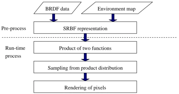
(10) density function (PDF).. Additionally, the approximated results are accurate enough to represent most features of the original data, and we can directly estimate the probability for importance sampling with the simple form of convolution by choosing the appropriate SRBF kernels. The potential benefits of SRBFs would make the importance sampling more efficient.. 1.2 System Overview The goal of this thesis is to demonstrate that the scattered SRBFs are appropriate to represent the HDR environment map and the complex measure BRDF data. With some useful properties of SRBF, we can easily apply the resulting representation in the Monte Carlo importance sampling technique. Finally, we show that the efficiency of importance sampling from product distribution can be improved with our sampling scheme. Figure 1 gives an overview of our new sampling technique for sampling the product of an environment map and a BRDF.. BRDF data. Pre-process. Run-time process. Environment map. SRBF representation. Product of two functions. Sampling from product distribution. Rendering of pixels Figure 1.1 System overview 3.

(11) 1.3 Thesis Organization The following chapters are organized as follows. In Chapter 2, we review some of the related works in sampling from environment maps, BRDFs and product distributions for global illumination. In Chapter 3, we briefly introduce the background of SRBFs and the advantages of scattered SRBFs. Chapter 4 presents how we fit scattered SRBFs to the BRDF data as well as the environment map, and how we generate sample directions at run-time efficiently. The implementation and results will be demonstrated in Chapter 5. Finally, the conclusions and future work are given in Chapter 6.. 4.

(12) Chapter 2 Related Works In this chapter, we survey previous works on importance sampling. The goal of global illumination is to solve the rendering equation which was first formulated by Kajiya [7]:. L ( x , ω o ) = Le ( x , ω o ) +. ∫ ρ (x , ω , ω )L (x , ω )(ω i. Ω. o. i. i. i. ⋅ n ) dω i ,. (1). where Li is the incident radiance, and ρis the BRDF. To evaluate this integral, it is common to use Monte Carlo approaches. They solve the integrals by computing the average of random samples of the integrand, accumulating these values and taking the average. Importance sampling is a variance reduction technique of Monte Carlo approaches. Most Monte Carlo approaches use importance sampling of either Li or ρ to solve the rendering equation. When sampling from BRDFs but do not take into account the lighting in the scene, they become inefficient with complex lighting. Similarly, when sampling only from environment lighting, it will be inefficient if the materials get increasingly specular. Thus, we attempt to sample from product of the BRDF and the illumination.. 2.1 BRDF Importance Sampling BRDF importance sampling is a technique to reduce the image variance in physically-based rendering. Its concept is to find the distribution based on the. 5.

(13) representation of BRDF. Simple analytical models such as diffuse, Phong, or generalized cosine models can be sampled analytically. Shirley demonstrated how to sample the traditional Phong BRDF model efficiently [20], Lafortune also presented importance sampling schemes for the modified Phong model [9]. Ward [24] showed the stochastic sampling method for the BRDF models composed of elliptical Gaussian kernels. Lafortune [10] used multiple cosine-lobes for representing the BRDF, he used non-linear fitting algorithm to fit sums of cosine-lobes to an analytical model or to actual measurements. Though this representation is simple and can be applied for Monte Carlo importance sampling efficiently, it is hard to approximate the complex BRDF by using his fitting process.. For measured BRDFs, Lalonde [11] used wavelets to represent the BRDF and proposed an importance sampling scheme by binary searching the tree constructed against the coefficients of each wavelet basis. Matusik [13] also used a wavelets representation of BRDF, and he presented a numerical sampling method based on wavelets analysis. Lawrence et al. [12] demonstrated an importance sampling method based on a factored representation. They reparameterized the BRDF by using half-angle [19], then used non-negative matrix factorization (NMF) twice to decompose the BRDF data for efficient importance sampling. Weng and Shih [25] represented the measured BRDF data with scattered SRBFs and estimated the probability distribution for importance sampling. Unfortunately, such approaches will not perform well for high-frequency illumination.. 2.2 Environment Map Importance Sampling Environment map importance sampling is another technique for increasing the. 6.

(14) efficiency of ray tracing based algorithms, under complex lighting captured in a high-dynamic range environment map. In some previous work, the environment maps are transformed into finite basis functions, such as wavelets [15] and spherical harmonics [17] [18] [21].. Some researchers have used importance sampling techniques to distribute samples according to the energy distribution in the environment map [1] [5] [8] [16]. The importance sampling is often implemented based on clustering algorithm or hierarchical tiling scheme. Similarly, such an approach performs poorly for highly specular surfaces, since samples chosen this way do not take specular lobe into account.. 2.3 Sampling from Product Distributions More recently, several researchers have worked on this problem by drawing samples from the product distribution of the illumination and the BRDF. These approaches produce high quality images with a small number of samples. Burke et al. [2] introduced a technique which is called bidirectional sampling. They take into account both the surface BRDF and energy of incident illumination in the sampling process. Two Monte Carlo algorithms for sampling from the product distribution are presented – one based on refection sampling and the other based on sampling-importance re-sampling (SIR).. Clarberg et al. [3] present a technique for importance sampling products of the BRDF and the illumination using a hierarchical wavelet representation. Their method is very efficient for measured BRDF data but requires significant precomputation for. 7.

(15) environment maps. Our approach use SRBFs instead of wavelets. Tsai and Shih [22] have shown this representation performs better than wavelets in data analysis. Furthermore, we can directly fit scattered SRBFs to BRDF data without re-parameterization. We also propose an efficient importance sampling method based on this representation. In the following chapters, we will describe how we represent the environment map and the measured BRDF data with scattered SRBFs and how we estimate the probability distribution for importance sampling.. 8.

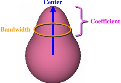
(16) Chapter 3 Background of SRBFs The spherical radial basis functions (SRBFs) are special radial basis functions defined on the unit sphere. Since SRBFs are defined in the spherical domain and have some properties, such as rotational invariance and positive definiteness, it makes SRBFs appropriate for modeling and analyzing spherical data without any artificial boundaries or distortions. In this chapter, we introduce the background of SRBFs that had been developed by previous researchers.. SRBFs is recognized as an circularly axis-symmetric reproducing kernel function defined on S m , which is the unit sphere in R m +1 . The kernel functions only depend on the spherical distance between unit vectors. Figure 3.1 gives an example of the 3D plot of a Gaussian SRBF.. Center Coefficient Bandwidth. Figure 3.1 3D plot of a Gaussian SRBF 9.

(17) Let η and ξ be two points on S m , and let θ(η,ξ) be the geodesic distance between η and ξ on S m , i.e. the arc length of the great circle joining the η and ξ. The kernel functions of SRBFs are depending on θ and can be expressed in the expansions of Legendre polynomials: ∞. G (cos θ ) = G (η ⋅ ξ ) = ∑ Gl Pl (η ⋅ ξ ) , l =0. (2). where Pl (η ⋅ ξ ) is the Legendre polynomials of degree l , and Gl is the Legendre coefficients satisfy the following two conditions:. ⎧Gl ≥ 0 ⎪∞ ⎨ . ⎪∑ Gl < ∞ ⎩ l =0 When all Gl are positive, a spherical function F (η ) can be represented in SRBF expansions as follows: N. F (η ) = ∑ Fk G (η ⋅ λ k ) .. (3). k =1. Thus, the SRBFs behave as reproducing kernels for interpolating F (η ) on S m . Figure 3.2 shows an example of SRBF representation for a spherical function F (η ) .. Figure 3.2 SRBF representation for a spherical function (k = 4) 10.

(18) Since SRBF can be expressed in terms of expansions in Legendre polynomials, it facilitates the convolution of two SRBFs. Based on the orthogonal property of Legendre polynomials in [-1, 1], the spherical singular integral is. (G1 ∗m G2 )(ξ1 ⋅ ξ 2 ) = ∫S. m. G (η ⋅ ξ1 )H (η ⋅ ξ 2 ) dω (η ) ∞. ωm. l =0. d m,l. = ∑ G1l G2l. Pl (ξ1 ⋅ ξ 2 ) ,. (4). where ω m is the total surface area of S m , d m ,l is the dimension of the space of order-l spherical harmonics on S m , and dω denotes the differential surface element on S m . Please refer to [14] and [6] for more details about spherical radial basis functions.. One example of SRBFs is the Gaussian SRBF kernel. The definition of Gaussian SRBF kernel is. G Gau (η ⋅ ξ ; λ ) = e − λ e λ (η ⋅ξ ) , λ > 0,. (5). where λ denotes the parameter called bandwidth and controls the coverage of the SRBF. We adopt Gaussian SRBF kernel as the kernel function for following reasons. First, Tsai and Shih [22] have proved that the convolution of two Gaussian SRBFs has a mathematically simple form for small m. It can be written as. (G. Gau 1. ). ∗m G2Gau (ξ1 ⋅ ξ 2 ; λ1 , λ2 ). ) −( + ⎛ m + 1⎞ = e λ 1 λ 2 ω m Γ⎜ ⎟ I m−1 ( r ⎝ 2 ⎠ 2. ⎛. ⎞. ) ⎜⎜ 2 ⎟⎟. m −1 2. (6). ⎝ r ⎠. where r = λ1ξ1 + λ 2ξ 2 . Second, the product of two Gaussian SRBFs is easy to evaluate. For more details about the proof of the Eq. 6, please refer to [22].. 11.

(19) Distribution of the SRBFs’ centers on the sphere affects the compression efficiency significantly. It would waste lots of basis kernels on the region without any data if we use uniform SRBFs to represent the data with sparse distribution. We can locate the SRBF kernels based on the data distribution on the sphere by using scattered SRBFs, i.e. adapting the center, bandwidth and coefficient of each basis. Therefore, scattered SRBFs can capture the feature of the original data with much fewer bases than those used in uniform SRBFs.. 12.

(20) Chapter 4 Off-Line SRBF Fitting Process Our approach contains two major processes, one is the pre-process and the other is the run-time rendering process. In the pre-process, we use scattered SRBF to represent the HDR environment maps and the measured BRDF data. In this chapter, we will introduce the non-uniform and non-negative SRBF fitting algorithm which we use to transform the HDR environment maps and the measured BRDF data into scattered SRBFs.. Weng and Shih [25] have presented an approach to fit the measured BRDF data using SRBFs representation. We use their approach to represent our BRDF data with SRBFs. On the other hand, we fit the HDR environment maps with SRBFs using non-uniform and non-negative optimization. There are three sets of parameters we want to optimize: the set of coefficients L , the set of centers Ξ 2 , and the set of bandwidth parameters Λ 2 . Our objective is to minimize the square error with the original data:. {L, Ξ 2 , Λ 2 } = arg min ∫S L(η i ) − L~ (η i ) {L ,Ξ 2 ,Λ 2 }. 2. nl ~ L (η i ) = ∑ Lk G (η i ⋅ ξ 2,k ; λ 2,k ). 2. dω (η i ),. (7). k =1. 13.

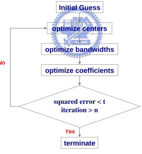
(21) Tsai and Shih [22] have presented a novel method to solve this objective function when modeling the lighting environment. We modify their method a little bit to make fitting result more suitable for importance sampling. In their fitting approach, the coefficients of each kernel basis are computed by ordinary least-squares (OLS) or regularized least-squares (RLS). Unfortunately, the coefficients would become negative in some situations when computing by OLS or RLS. We must constrain all coefficients to be positive because we need to use coefficients to estimate the probability distribution. Therefore, we use L-BRFS-B solver [26] to optimize the coefficients. Figure 4.1 gives a flow chart of fitting process.. Initial Guess optimize centers optimize bandwidths No. optimize coefficients. squared error < t iteration > n Yes. terminate. Figure 4.1 Flow chart of fitting process. 14.

(22) The non-uniform and non-negative SRBF fitting algorithm composes of follow main steps: 1. Using L-BFGS-B solver to optimize the set of centers from a given initial guess or the results of the previous iteration. 2. Using L-BFGS-B solver to optimize the set of bandwidth parameters and the set of coefficients respectively. 3. The process is terminated if the difference of squared errors between current and previous iteration are less than a threshold, or the count of iteration exceeds a user-defined threshold.. This process is one kind of non-linear optimization. The fitting results are highly dependent on the initial guess, i.e. the initial guess would dominate the accuracy of the representation. Tsai and Shih [22] also have presented a reasonable guess based on some heuristics to decrease approximation errors and accelerate the computation. The principle of their initial guess is to make the initial centers of each kernel basis locate at all local peaks of the original data as close as possible, and to estimate a reasonable bandwidth according to the coverage of each initial center. Based on this principle, they generate lots of candidate guesses sorted by the coverage-weighted intensity, and then attempt to choose guesses which avoid the initial centers gathering in local area. This scheme works well for the data with high dynamic range property. For more detail about initial guess, please refer to [22].. After fitting process, we have represented the HDR environment map with SRBFs: K. L(η i ) ≈ ∑ Fk G (η i ⋅ ξ k ; λk ) ,. (8). k =1. 15.

(23) where L(η i ) is the incident radiance, G is the SRBF kernel function, ξ k is the center of basis on unit sphere, λ k is the bandwidth of the basis, Fk is the basis coefficient, and K is the number of the basis function. Figures 4.2 and 4.3 show the two reconstructed results of HDR environment maps obtained using SRBFs representation with 300 basis functions.. Similarly, the measured BRDF data is represented in scattered SRBFs for each fixed outing direction: K. ρω (ωi ) ≈ ∑ Fk G (ωi ⋅ ξ k ; λk ) , o. (9). k =1. where ρ ωo (ω i ) is the BRDF with a fixed outgoing direction ω o , and G is the SRBF kernel function.. (a) Reference. (b) Reconstructed from SRBFs. Figure 4.2 HDR environment map – St. Peter’s Basilica. 16.

(24) (a) Reference. (b) Reconstructed from SRBFs. Figure 4.2 HDR environment map – Uffizi Gallery. 17.

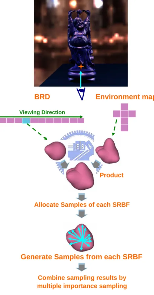
(25) Chapter 5 Run-Time Rendering Process In the run-time rendering process, we first evaluate the product of the two SRBFs. Then we determine how many samples should be taken from each SRBF. Since each SRBF kernel can be taken as some kind of the density distribution function, we can easily generate samples based on the probability density function (PDF) calculated from each SRBF. Finally, we combine the sampling results with multiple importance sampling technique presented by Veach and Guibas [23].. Figure 5.1 illustrates the flow of our run-time rendering process. When the view ray hits the object in the scene, we first calculate the product of the BRDF and the environment map represented in SRBFs. Next, we determine the number of the samples of each SRBF according to its integral. Then we generate samples from each SRBF and combine the results by multiple importance sampling technique.. The following sections are organized as follows. In Section 5.1 we describe how we calculate the product of two SRBFs. In Section 5.2, we briefly introduce the multiple importance sampling technique. Finally, we describe how to determine the number of samples of each SRBF kernel and how to generate samples from each SRBF kernel.. 18.

(26) BRD. Environment map. Viewing Direction. Product. Allocate Samples of each SRBF. Generate Samples from each SRBF Combine sampling results by multiple importance sampling Figure 5.1 Run-time rendering process. 19.

(27) 5.1 Product of the Illumination and the BRDF As mentioned before, we take Gaussian SRBF as the kernel function for some benefits. One reason is that the product of two Gaussian SRBFs is easy to calculate. Ignore the normalized term, the product of two Gaussian SRBFs is. F1e λ1 (η ⋅ξ1 ) ⋅ F2 e λ2 (η ⋅ξ 2 ) = F3e λ3 (η ⋅ξ3 ) F3 = F1 ⋅ F2. λ3 = λ1ξ1 + λ2ξ 2. (10). λ ξ + λ2ξ 2 ξ3 = 1 2 λ3. where F3 is the coefficient of product result, λ3 is the bandwidth of product result, and ξ 3 is the center of product result. The product of the BRDF and the illumination is shown as follows: M. L(ωi )ρ ωo (ωi ) ≈ ∑ F m =1. illu min ation m. N. G (ωi ⋅ ξ m ; λm )∑ Fnbrdf G (ωi ⋅ ξ n ; λn ) (11) n =1. where L(ω i ) is the incident radiance and ρ ωo (ω i ) is the BRDF with a fixed outgoing direction ω o .. After calculating the product of two SRBFs, the number of basis functions becomes M × N . If we take the whole basis functions to generate the samples, it will cause considerable computation cost. Thus, we reserve these basis functions which contain large coefficients and prune the basis functions that contain small coefficients. Since most of energy is distributed in a few basis functions that contain large coefficients, a good approximation for original data is obtained even if only the n largest coefficients are kept.. 20.

(28) 5.2 Multiple Importance Sampling After calculating the product of the BRDF and the environment map, it is desirable to generate rays distributed according to the density of the product. We are interested in evaluating the integral of the incident illumination for a fixed outgoing direction ω o located at x with normal n ,. L (x , ω o ) =. ∫. Ω. L i ( x , ω i )ρ ( x , ω i , ω o )(ω i ⋅ n )V ( x , ω i ) d ω i .. (12). The Monte Carlo estimator for the above integral can be written as:. L( x, ωo ) = ∫ Li (x, ωi )ρ ( x, ωi , ωo )(ωi ⋅ n )V ( x, ωi ) dωi Ω. . 1 n ⎡ Li ( x, ωi )ρ ( x, ωi , ωo ) ⎤ ≈ ∑⎢ ⎥ (ω s ⋅ n )V ( x, ω s ) n s =1 ⎣ γ (ω s | ωo ) ⎦. (13). However , it is hard to construct a single PDF γ (ω s | ω o ) that follows the shape of the complex product of the BRDF and the illumination. We adopt a technique for importance sampling presented by Veach and Guibas [23] called multiple importance. sampling. By combining several potentially good estimators, this technique makes Monte Carlo integration more robust. These estimators calculated by different PDFs may have different qualities in different regions of the integration domain. Veach and Guibas make a weighted-average of all estimators where the weights depend on the sampling positions. If we want to evaluate the integral of f (x ) :. ∫ f (x) dx , Ω. and we have n different estimators, the combined estimator is then given by n. 1 F =∑ i =1 ni. ni. ∑ wi (X i, j ) j =1. f (X i , j ). p i (X i , j ). (14). where pi is the PDF for each estimator, ni denotes the number of samples from. 21.

(29) pi , X i , j are the samples from pi , for j = 1,..., ni , and all samples are assumed to be independent. wi is the weighting function which satisfies the following two conditions:. ⎧n ⎪∑ wi ( x ) = 1 ⎨ i =1 ⎪w ( x ) = 0 whenever ⎩ i. pi ( x ) = 0. .. (15). Then, the expected value of the combined estimator F would be equal to the integral of f (x ) which we want to evaluate.. So far, we have represented the product of the BRDF and the illumination using scattered SRBFs. Now we apply this technique to importance sampling from product distribution, and the Equation (13) would become:. ∫ L (x,ω )ρ(x,ω ,ω )(ω ⋅ n ) V (x,ω ) dω ⎡ n p (X ) ⎤ ⎡ L (x, X )ρ(x, X 1 ≈ ∑ ∑⎢ ⎥⎢ ( ) n n p X p (X ) ⎣⎢ ∑ ⎦⎥ ⎢⎣ i. Ω. i. i. ni. n. i =1. i j =1. o. i. k. i. k. i. i, j. k. i. i. i, j. i. i, j. i. i, j. i, j. ,ωo )⎤ (16) ⎥ (X i, j ⋅ n ) V (x, X i, j ) ⎥⎦. where n is the number of SRBFs, ni denotes the number of samples from each SRBF, and pi is the PDF calculated from each SRBF kernel function, for i = 1,..., n .. X i , j are the samples from each SRBF kernel function, for j = 1,..., ni .. There are two issues to compute the Equation (16) in run-time rendering process. One is how to determine ni , the number of samples should be taken from each SRBF kernel, the other is how to generate X i , j , the sampling directions distributed according to each SRBF kernel. These two issues will be discussed in the following section.. 22.

(30) 5.3 Sampling Algorithm We now describe how to use our representation for multiple importance sampling. Intuitively, each scattered SRBF covers a part of the entire product region. Although there would be two or more SRBFs overlap in the same regions, we can still gather the intensity of multiple sampling directions within a pixel using multiple importance sampling approach.. As mentioned before, we first calculate the product of the BRDF and the environment map for a given viewing direction in the run-time rendering process. Then, we have multiple SRBF kernel functions, now we should decide how many samples should be taken from each SRBF kernel. Let’s recall that SRBF is defined on the unit sphere, and its integral is easy to be calculated by using the spherical singular integral property of SRBF. The integral of each SRBF can be taken as its total energy gathered from all directions. Therefore, it is straightforward to allocate samples according to the ratio of the integral of each SRBF to the sum of all SRBFs’ integrals. Furthermore, we want to allocate more samples in the SRBFs which contain higher energies. Thus, we emphasize the energy by squaring the influence of integral. The probability of choosing the SRBF l for each sample is given by:. P(l ) =. Ii n. ∑ Ii. .. (17). i =1. We calculate a 1D CDF over l from these probabilities. In the dispatching process, we initially generate a uniform variable in [0, 1] and jitter this variable with a random number for each sample. Then, we traverse the CDF to determine where the sample should be taken from.. 23.

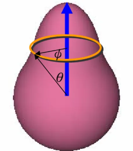
(31) Next, we generate a sample direction in each SRBF kernel by sequentially selecting the elevation angle θ and the azimuth angle ψ defined on the plane whose normal is parallel to the SRBF kernel’s center (Figure 5.2).. ψ θ. Figure 5.2 The elevation angle and the azimuth angle defined against SRBF. For the elevation angle θ, we use metropolis random walk algorithm to generate samples with a desired density. It should be noted that the SRBF kernel itself only describes 1D density, while the desired density of sampling is the density over the sphere. Therefore, when we select the elevation angle θ by this approach, we should consider the influence of the circumference around the center of SRBF kernel especially. For the azimuth angle ψ, each SRBF kernel is symmetric against the vector that defined by its center and the origin of the unit sphere. Therefore, the distribution of azimuth angle ψ is uniform, and we can simply generate a random number in [0, 2π] to evaluate ψ.. 24.

(32) Chapter 6 Implementation and Results This chapter demonstrates the results of our new sampling technique. All results are generated on an AMD Athlon64 FX-60 PC with NVIDIA GeForce 7900 GTX. We illustrate the rendering results of several measured BRDF data and complex HDR environment map.. We compare our method to SRBFs-based BRDF importance sampling presented by Weng and Shih [25], i.e., not using the SRBF product. Figures 6.1~6.3 show the comparisons between BRDF importance sampling and our approach with varying number of samples. The Buddha model in ‘Grace Cathedral’ rendered with different measured BRDF data. From Figures 6.1 to 6.3, the materials are ‘Garnet Red’, ‘Krylon Blue’, and ‘Cayman’ measured by Cornell University. From (a) to (e) is the sampling results from SRBF product with vary different number of samples. And (f) is the rendered results using SRBFs-based BRDF importance sampling. Performing the SRBFs product sampling in the run-time process obviously adds some overhead. In our current implementation, our method increase 40 percent computation time than SRBFs-based BRDF importance sampling for equal number of samples. But the quality of the rendered images with our method is much better than with SRBFs-based BRDF importance sampling.. 25.

(33) (a) 10 samples. (b) 40 samples. (d) 80 samples. (b) 100 samples. (c) 60 samples. (c) 100 samples (BRDF). Figure 6.1 Sampling results with material ‘Garnet Red’. 26.

(34) (a) 10 samples. (b) 40 samples. (d) 80 samples. (b) 100 samples. (c) 60 samples. (c) 100 samples (BRDF). Figure 6.2 Sampling results with material ‘Krylon Blue’. 27.

(35) (a) 10 samples. (b) 40 samples. (d) 80 samples. (b) 100 samples. (c) 60 samples. (c) 100 samples (BRDF). Figure 6.3 Sampling results with material ‘Cayman’. 28.

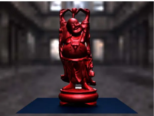
(36) We also render complex scene with three different measured BRDF data and two complex HDR environment maps with 60 samples per pixel in figures 6.4~6.7. We represent each BRDF measurements in scattered SRBFs with 5 Gaussian kernels and each environment map in scattered SRBFs with 100 Gaussian kernels. After computing the products, we reserve 100 Gaussian kernels to generate samples.. Figure 6.4 A ‘GarnetRed’ Buddha and a ‘Cayman’ plane in ‘Uffizi Gallery’ HDR environment. 29.

(37) Figure 6.5 A ‘KrylonBlue’ Buddha and a ‘Cayman’ plane in ‘Uffizi Gallery’. Figure 6.6 A ‘KrylonBlue’ Buddha and a ‘Cayman’ plane in ‘St. Peter’s Basilica’ 30.

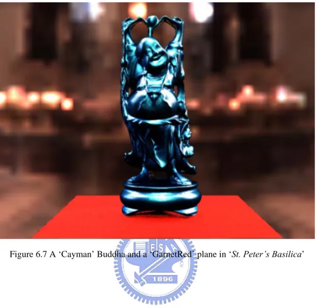
(38) Figure 6.7 A ‘Cayman’ Buddha and a ‘GarnetRed’ plane in ‘St. Peter’s Basilica’. 31.

(39) Chapter 7 Conclusions and Future Works We propose a new technique for importance sampling products of the BRDF and the illumination. Based on the scattered SRBFs representation, we can generate samples following the desired densities efficiently. Furthermore, this representation is easy to be applied to the multiple importance sampling technique. Finally, we use our sampling scheme to render scenes with multiple complex materials and HDR environment maps. Although our approach would increase the computation time of density estimations, we can generate much smaller samples than the approach considering BRDF only to get the same rendering quality. And we reduce the number of visibility tests required to obtain good image quality.. Compared with previous methods, SRBF representation can significantly decrease pre-computed data storage. For example, wavelet importance sampling presented by Clarberg et al. [3] requires significant precomputation for environment maps when rotating lighting environment. In order to get a smooth result, they must bilinearly interpolate between the four nearest wavelets in the environment map. Since a SRBF is rotation-invariant function, rotating functions in SRBF representation is as straightforward as rotating the centers of SRBF. We can simply get correct SRBFs by one rotation operation.. 32.

(40) Our approach achieves low variance in non-occluded regions. However, the resulting images still have noise in partially occluded regions as our approach does not take visibility into account during the sampling process. On the other hand, the major computation cost for ray tracing is the visibility testing. In the future, we would like to generate samples smarter based on some heuristic approach. We would improve the efficiency of importance sampling and the quality of rendered images.. 33.

(41) References [1] Agarwal, S., Ramamoorthi, R., Belongie, S., and Jensen, H. W. 2003. Structured Importance Sampling of Environment Maps. ACM Transactions on Graphics 22, 3, 605-612. [2] Burke, D., Ghosh, A., Heidrich, W. Bidirectional Importance Sampling for Direct Illumination. In Eurographics Symposium on Rendering, 147-156. [3] Clarberg, P., Jarosz, W., Akenine-Moller, T., Jenson, H.W. 2005. Wavelet Importance Sampling: Efficiently Evaluating Products of Complex Functions. ACM Transactions on Graphics 24, 3, 1166-1175. [4] Claustres, L., Paulin, M., and Boucher, Y. 2003. BRDF Measurement Modeling using Wavelets for Efficient Path Tracing. Computer Graphics Forum 22, 4, 701-716. [5] Cohen, J., and Debevec, P., 2001. LightGen, HDRShop plugin. [6] Freeden, W., Gervens, T., and Schreiner, M. 1998. Constructive Approximation on the Sphere. Oxford University Press. [7] Kajiya, J. T. 1986. The Rendering Equation. In SIGGRAPH 86, 143-150. [8] Kollig, T., and Keller, A. 2003. Efficient Illumination by High Dynamic Range Images. In Eurographics Symposium on Rendering, 45-50. [9] Lafortune, E. P., and Willems, Y. D. 1994, Using the Modified Phong Reflectance Model for Physically Based Rendering. Technical Report RP-CW-197, Department of Computing Science, K.U. Leuven, 1994. [10] Lafortune, E. P. F., Foo, S.-C., Torrance, K. E., and Greenberg, D. P. 1997. Non-Linear Approximation of Reflectance Functions. In SIGGRAPH 97, 117-126. [11] Lalonde, P. 1997. Representations and Uses of Light Distribution Functions. PhD thesis, University of British Columbia. [12] Lawrence, J., Rusinkiewicz, S., and Ramamoorthi, R. 2004. Efficient BRDF Importance Sampling using a Factored Representation. ACM Transactions on Graphics 23, 3, 496-505. [13] Matusik, W., Pfister, H., Brand, M., and McMillan, L. 2003. A Data-Driven Reflectance Model. ACM Transactions on Graphics 22, 3, 759-769. 34.

(42) [14] Narcowich, F. J., and Ward, J. D. 1996. Nonstationary Wavelets on the m-Sphere for Scattered Data. Applied and Computational Harmonic Analysis 3, 4, 324-336. [15] Ng, R., Ramamoorthi, R., Hanrahan, P. 2003. All-Frequency Shadows using Non-linear wavelet lighting approximation. ACM Transactions on Graphics 22, 3, 376-381. [16] Ostromoukhov, V., Donohue, C., and Jodoin, P.-M. 2004. Fast Hierarchical Importance Sampling with Blue Noise Properties. ACM Transactions on Graphics 23, 3, 488-495. [17] Ramamoorthi, R., Hanrahan, P. 2001. An Efficient Representation for Irradiance Environment Maps. In Proc. of ACM SIGGRAPH 01, 497-500. [18] Ramamoorthi, R., Hanrahan, P. 2002. Frequency Space Environment Map Rendering. In Proc. of ACM SIGGRAPH 02, 517-526. [19] Rusinkiewicz, S.M. 1998. A New Change of Variables for Efficient BRDF Representation. In Eurographics Workshop on Rendering, 11-22. [20] Shirley, P. S. 1991. Physically Based Lighting Calculations for Computer Graphics. PhD thesis, University of Illinois at Urbana-Champaign. [21] Sloan, P., Kautz, J., Snyder, J. 2002. Precomputed Radiance Transfer for Real-Time Rendering in Dynamic, Low-Frequency Environments. In Proc. of ACM SIGGRAPH 02, 527-536. [22] Tsai, Y. T., and Shih, Z. C. 2006. All-Frequency Precomputed Radiance Transfer using Spherical Radial Basis Functions and Clustered Tensor Approximation. ACM Transactions on Graphics, 25, 3, 967-976. [23] Veach, E., and Guibas, L. 1995. Optimally Combining Sampling Techniques for Monte Carlo Rendering. In SIGGRAPH 95, 419-428. [24] Ward, G. J. 1992. Measuring and Modeling Anisotropic Reflection. In SIGGRAPH 92, 265-272. [25] Weng, S. C., and Shih, Z. C. 2006. An Efficient BRDF Importance Sampling Method for Global Illumination. Master thesis, College of Computer Science, National Chiao Tung University. [26] Zhu, C., Byrd, R. H., Lu, P., and Nocedal, J. 1997. Algorithm 778: L-BFGS-B: Fortran Subroutines for Large Scale Bound-Constrained Optimization. ACM Transactions on Mathematical Software 23, 4, 550-560. 35.

(43)