A MODEL-REFERENCE CONTROL-STRUCTURE USING A FUZZY NEURAL-NETWORK

(1)

E L S E V I E R Fuzzy Sets and Systems 73 (1995) 291-312

N l Z Z Y

sets and systems

A model reference control structure using a fuzzy neural network

Y i e - C h i e n C h e n , C h i n g - C h e n g T e n g *

Institute of Control Engineering, National Chiao-Tung University, Hsinchu, Taiwan Received May 1994; revised August 1994

Abstract

In this paper, we present a design method for a model reference control structure using a fuzzy neural network. We study a simple fuzzy-logic based neural network system. Knowledge of rules is explicitly encoded in the weights of the proposed network and inferences are executed efficiently at high rate. Two fuzzy neural networks are utilized in the control structure. One is a controller, called the fuzzy neural network controller (FNNC); the other is an identifier, called the fuzzy neural network identifier (FNNI). Adaptive learning rates for both the FNNC and FNNI are guaranteed to converge by a Lyapunov function. The on-line control ability, robustness, learning ability and interpolation ability of the proposed model reference control structure are confirmed by simulation results.

Keywords: Fuzzy logic; Neural network; Fuzzy neural network; Model reference control

1. Introduction

Recently, fuzzy neural network control systems have been extensively studied. F o r instance, Lin [12] proposed a general neural network model for a fuzzy logic control and decision system, which is trained to control an unmanned vehicle by combining unsupervised and supervised learning. Horikawa et al. [6] presented a fuzzy neural network that learned expert control rules, while Lee [10] combined Barto's adaptive neurons with a fuzzy logic controller to deal with the pole balancing problem. However, in all of these systems a teacher responsible for training is required. Furthermore, adaptation to changes in the environment is not provided for.

The structure of the fuzzy neural network presented by Lin [12] consists of five layers, which is a little complicated. The proposed fuzzy neural network is a slight modification of that in [12, 6]. Thus, we have a four-layer fuzzy neural network structure and the calculation of the proposed system is simpler than H o r i k a w a ' s T Y P E - I F N N . The main advantages of the structure we adopted are (1) the ability to learn from experience, (2) a high computation rate, (3) the easily understandable manner in which knowledge acquired is expressed and (4) a high degree of robustness and fault tolerance.

* Corresponding author.

(2)

292 E-C. Chert, C.-C. Teng / Fuzzy Sets and Systems 73 (1995) 291-312

In the conventional adaptive control literature, there are two distinct adaptive control categories: (1) direct adaptive control and (2) indirect adaptive control [13]. In direct adaptive control, the parameters of the controller are directly adjusted to reduce some norm of the output error (between the plant and the reference model). On the other hand, in indirect adaptive control, the parameters of the plant are estimated and the controller is chosen assuming that the estimated parameters represent the true values of the plant parameters. In the control system, if the plant is unknown, many people simply ignore the sensitivity and use the direct control approach.

In this paper, we propose a model reference control structure that uses a fuzzy neural network. The proposed model reference control structure belongs to indirect adaptive control, and a controlled plant is identified by the fuzzy neural network identifier (FNNI), which provides information about the plant to the fuzzy neural network controller (FNNC). This structure is a real adaptation system that can learn to control a complex system and adapt to a wide range of variations in plant parameters. Unlike most other adaptive learning neural controllers [1, 2, 5, 9, 11, 13, 14, 17], the FNNC presented in this paper is based not only on the theory of neural network computing but also on that of fuzzy logic I-3].

Though the proposed control scheme is a slight modification of those in [4, 13], we believe that our structure is more reasonable for a fuzzy logic control system. Since the place for the reference model (RM) in the proposed system is specially considered, the FNNC is designed such that the actual output of the system will track the desired output of the reference model. Moreover, we can simply take the error (between the actual output and the desired output) and the change in this error as the inputs for FNNC.

We also apply some of the theorems in [9] to develop convergence theorems for both FNNI and FNNC. To guarantee convergence and for faster learning, an analytical method based on the Lyapunov function is proposed to find the adaptive learning rates for FNNI and FNNC. This paper is organized as follows. In Section 2, a simple fuzzy-logic based neural network system is studied. Section 3 presents a model reference adaptive control structure using a fuzzy neural network. In this structure, the control action is updated on-line using the information stored in a fuzzy neural network identifier (FNNI). The convergence of the FNN-based system is investigated in Section 4. In Section 5, examples are presented to illustrate the performance of the control system. Concluding remarks are given in Section 6.

2. Fuzzy neural network

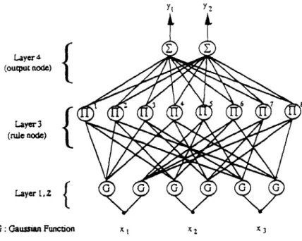
In this section we will present a simple fuzzy logic system implemented by using a multilayer feedforward neural network. A schematic diagram of the proposed fuzzy neural network (FNN) structure with three input variables, two term nodes for each input variable, two output nodes, and eight rule nodes is shown in Fig. 1. The system consists of four layers. Nodes in layer one are

input nodes

which represent input linguistic variables. Nodes in layer two are

membership nodes

which act like membership functions. Each membership node is responsible for mapping an input linguistic variable into a possibility distribution for that variable. The rule nodes reside in layer three. Taken together, all the layer three nodes form a fuzzy rule base. Layer four, the last layer, contains the output variable nodes.

The links between the membership nodes and the rule nodes are the antecedent links and those between the rule nodes and the output nodes are the consequence links. For each rule node, there is at most one antecedent link from a membership node of a linguistic variable. Hence there are I-Ii I T(x~)I rule nodes in the proposed FNN structure. Here [ T(x~)l denotes the number of fuzzy partitions of input linguistic variable x~. Moreover, all consequence links are fully connected to the output nodes and interpreted directly as the strength of the output action. In this way, the consequence of a rule is simply the product of the rule node output, which is the firing strength of the fuzzy rule and the consequence link. Thus, the overall net output is treated as a linear combination of the consequences of all rules instead of the complex composition, a rule of inference and the defuzzification process. This fuzzy neural network is a slight modification of the network

(3)

Yt Y2 Layer (outaut nc~) Layer3 (mJ, e node) Layer t,r-

{

G : Camssum Fun~on

Y.-C Chen, C-C Teng / Fuzzy Sets and Systems 73 (1995) 291-312 293

x t x 2

Fig. 1. Schematic diagram of a fuzzy neural network.

reported by Lin [12]. The interested readers are referred to Lin [12] for a more detailed explanation of the network.

2.1. Reasoning method

For an n-input-one-output system, let xi be the ith input linguistic variable and define ~k as the firing strength of rule k, which is obtained from the product of the grades of the membership functions #A,,(xi) in the antecedent. If Wk represents the kth consequence link weight, the inferred value y* is then obtained from the weighted sum of its inputs, i.e.Y.k WkCtk. The proposed fuzzy neural network realizes the inference as follows

R k: IF xl is Ak(xl), ... ,and xn is Ak(x,), then y = Wk, k = 1,2 . . . m

y * = ~ ~kWk, ~k = ~ #A'.(X,).

k = l i = 1

The reasoning method is a variation of the reasoning method introduced by Sugeno [15], in which the consequence of a rule is a function of input variables. For the proposed FNN, this function is replaced by a constant value and a different defuzzification process is used.

2.2. Basic nodes operation

Next, we shall indicate the signal propagation and the basic function of every node in each layer. Layer 1: input layer

For the jth node of layer 1, the net input and the net output are represented as: n e t ] = w ~ ' x ~ i = j , yl. = f j l ( n e t ) ) = n e t ~

1

(4)

294 Y.-C. Chen, C.-C. Teng / Fuzzy Sets and Systems 73 (1995) 291-312

Layer 2: membership layer

In this layer, each node performs a membership function. The Gaussian function, a particular example of radial basis functions, is adopted here as a membership function. Then,

( X2 -- mij) 2

y2 =fj2(net 2) = exp(net2),

net f

= l l a o ( m i j , aij) ~- (o./j)2 '

where m o and

tTij

are, respectively, the mean (or center) and the variance (or width) of the Gaussian function

in the jth term of the ith input linguistic variable x 2.

Layer 3: rule layer

The links in this layer are used to implement the antecedent matching. The matching operation or the fuzzy AND aggregation operation is chosen as the simple P R O D U C T operation instead of the MIN operation. Then, for the jth rule node

net~

=

f i 3 3

wox, '

y3 =fj3(net~)= net~,

i

where w~ is also assumed to be unity.

Layer 4." output layer

Since the overall net output is a linear combination of the consequences of all rules, the net input and output of the jth node in this layer are simply defined by

n e t ; = ~ .

wox, ,

" "

y? = f~'(net?) = net~,

i

where the link weight w~ is the output action strength of the jth output associated with the ith rule.

Note that

neti, J~

are the summed net input (or activation level) and activation function of node j,

respectively, and the superscript denotes the layer number. From the above configuration, by modifying the centers and widths of layer 2 and the link weights of layer 4, the membership functions can be fine-tuned and all the consequence strengths of fuzzy rules could be identified respectively. The learning process to train the proposed fuzzy neural network will be discussed in the following section.

2.3. Supervised gradient descent learning

The adjustment of the parameters in the proposed F N N can be divided into two tasks, corresponding to the IF (premise) part and THEN (consequence) part of the fuzzy logical rules. In the premise part, we need to initialize the center and width for Gaussian functions. To determine these initial terms, a self-organization- map (SOM) [8] and fuzzy-c-means (FCM) [16] are commonly used. Another simple and intuitive method of doing this is to use normal fuzzy sets to fully cover the input space. Since the final performance will depend mainly on supervised learning, we choose normal fuzzy sets in this paper. In the consequence part, the parameters are output singletons. These singletons are initialized with small random values, as in a pure neural network.

A supervised learning law is used to train the proposed model. The basis of this algorithm is simply gradient descent. The derivation is the same as that of the back-propagation learning law. By recursive applications of the chain rule, the error term for each layer is first calculated. The adaptation of weights to the corresponding layer is then given. Next, we will begin to derive the learning law for each layer in the feedbackward direction.

(5)

Y.-C Chen, C - C Teng / Fuzzy Sets and Systems 73 (1995) 291-312 295

L a y e r 4: I f the cost function to be minimized is defined as

= - = :~ Z (de - f j a ( n e t ) ) ) 2 ,

J J

where d 4 is the desired output and Y4 is the current output of the jth output node, the error term to be propagated is given by

- d E - d E d f j 4 4

64 = dnet 4 - dfj 4 dnet¢ = d4 - yj

then, the weight w 4 is updated by the amount

d E dE dfj" dnet 4 = (d 4 _ y~). yi3 = j~.. y31"

Aw - dw = d 'dnet,"

L a y e r 3: Since the weights in this layer are unity, none of them is to be modified. Only the error term needs

to be calculated and propagated.

- d E - dE d f j 3 d E dnet 4 4 4

6 J 3 = ~ = ~f~ ffn-~-etj3=-- k~dnet 4 dy--?j

=~k 6kWjk"

L a y e r 2: The multiplication operation is done in this layer. The adaptive rule for mij and aq are as follows.

First, the error term is computed,

- - d E - d E d ~ 2

fi} = ~ = dffl dnet f

= _ ( k ~ dE dnetak ~ . dfj 2 -

dnetak dy2 ] ~ - - ( ~ k 6 ~ i ~ j Y 2 ) "exp(net2)

= 6k Yi "Yj = 6k "Yk,

i ~ j / k

where the subscript k denotes the rule node in connection with the jth node in Layer 2. Then, the adaptive rule of m~j is

d E _ dE dnet 2 2 2(y~ - mij)

Amij = dm 0 dnet] dm 0 = 6j -tr~

and the adaptive rule of tr 0 is

d E dE cOnet 2 2(y/1 -- m i j ) 2

(6)

296 Y.-C Chen, C-C Teng / Fuzzy Sets and Systems 73 (1995) 291-312

This completes the derivation of the supervised gradient descent learning algorithm. In the following section, the proposed FNN will be employed as a controller and an identifier. A controlled plant is identified by the FNNI, which provides information about the plant to the FNNC.

3. Model reference control structure using F N N

Fuzzy logic systems and neural networks can be exploited to emulate the capabilities of the human brain. Merging these two different disciplines makes it possible to develop a unified system that reasons and learns by experience and adapts to changes in plant parameters.

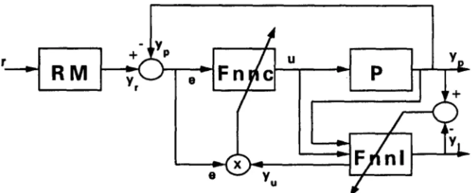
Fig. 2 shows the proposed model reference control structure using a fuzzy neural network. The proposed control scheme must perform two major tasks: (1) system identification and (2) plant control. The former is achieved by using the proposed fuzzy neural network identifier (FNNI) to estimate the dynamics of the controlled plant. The latter is achieved by using the proposed fuzzy neural network controller (FNNC) to generate the control signals.

The control action issued by the FNNC is updated by observing the controlled results through the FNNI. The adaptive FNNC has many useful features: (1) it can self-organize its control law during the control process; (2) it is able to make inferences using the control law encoded in the FNNC; (3) it is capable of high-speed parallel computation; and (4) it adapts automatically to changes in plant parameters.

In this paper the control law learned by the FNNC can be expressed explicitly in linguistic cause-and-effect rules, while a conventional neural controller can only encode the control law implicitly in variable weights. The structure of Fig. 2 is a slight modification of those in I4, 13].

3.1. Overall structure of the system The fuzzy neural network identifier: FNNI

The purpose of the FNNI is to mimic the dynamic characteristics of the controlled plant. Training of the FNNI is similar to plant identification except that the plant identification here is done automatically by a fuzzy neural network which is capable of modelling nonlinear plants [3]. The FNNI is trained by the above algorithm to predict the state vector of the plant y~, with the actual value of the state of the plant yp used as the desired response. The training process ceases when the error signal between y~ and yp becomes small enough. If changes in the system parameters or in the environment occur, the FNNI is triggered on again to begin relearning.

R M

Fnp/ c u

_1

I

(7)

E-C Chen, C-C. Teng / Fuzzy Sets and Systems 73 (1995) 291-312 297

The f u z z y neural network controller: F N N C

The fuzzy neural network here serves as a feedback controller. The F N N C is expected to approximate an optimal control surface. The optimal control surface is encoded in the form of fuzzy rules, which are represented by the interconnection weights embedded in the FNNC. Thus the weights can be modified to establish different control rules. As time goes by and the system accumulates more experience, it learns to control the plant more effectively. A controlled plant is identified by the FNNI, which provides information about the plant to the FNNC.

The reference model: R M

The reference model specifies the desired performance of the control system. The controller is designed such that the actual output of the system will track the desired output of the reference model. This goal can be achieved by minimizing e = (y~ - yp).

Note that our structure is different from that in [13], in which the reference model is placed on the upper side. We believe that our structure is more reasonable for a fuzzy system since we can simply take the error (between actual output and desired output) and the change in this error as the input for FNNC.

3.2. Training the F N N I and F N N C

Let the cost function, El, for training pattern k be proportional to the sum of the square of the difference between the plant output y ( k ) and the actual output yl(k) of FNNI, and let El be defined by

E, = ½[y(k) - yl(k)] 2. (1)

Then the gradient of error in Eq. (1) with respect to an arbitrary weighting vector W~ e ~ " becomes

dE1 dei(k) , , , dyi(k) dOl(k)

dW---~ll = el(k) d W ~ - efltc~ dW~ = - el(k) 8W---~' (2)

where ei(k) = y(k) - yi(k) is the error between the plant and the F N N I response. Ol(k) is the actual output of the identifier (FNNI).

The weight can be adjusted using a gradient method: dEi )

W~(k + 1) = Wl(k) + AWl(k) = Wi(k ) + r h - - ~ , (3)

where t/! is a learning rate.

Let the cost function, Ec, for training pattern k be proportional to the sum of the square of the difference between the desired output yr(k) of the reference model and the plant output y(k), and let Ec be defined by

Ec = ½ [y,(k) - y(k)] 2.

(4)

Then the gradient of error in Eq. (4) with respect to an arbitrary weighting vector W c e 9~" becomes dEc "k' dec(k) , , , dy(k)

b-ff-~ =ect J dwc =-ectK~-b-ff-d~

, , , dy(k) du(k)

= -- ectK}~--U-~ d W c - - = - e c ( k ) y ~ ( k ) ' - -

dOc(k)

(8)

298 Y.-C. Chen, C - C . Teng / Fuzzy Sets and Systems 73 (1995) 291-312

where ec(k) = yr(k) - y(k) is the error between the actual plant and the desired reference output, Oc(k) is the output of the controller (FNNC) and S = yu(k) = t3y(k)/au(k) is the plant sensitivity.

The weight can be adjusted using a gradient method.

(

Wc(k + 1) = Wc(k) + AWc(k) = Wc(k) + qc - 0--WccJ" (6)

where r/c is a learning rate.

The plant sensitivity can be computed as follows:

, ~ ( 4 ) c3yj _ ~,,,.,~j c~ui Oui - ~ ( 4 ) ( 3 ) Ri ~ ( J l a j . ,~f~(3)'~ _{WVlka ~ ~. R,}

= Z ~ao~22 ~u, )

Z w~j.

R~ ' dORa J ~ ' k a = Z w . i " =

a = l k = l C30it2k , ~Ui 3 Z Waj"

.

0o, ,t.

{

= • '-'bL "-~-U/J • = Z W.~ • 0 ~ , "~ --2) ( ~ i k ) 2 j , (7)

a = l i a = l

where rnik and aik are, respectively, the mean (or center) and the variance (or width) of the Gaussian function in the kth term of the ith input linguistic variable ui. The superscript denotes the layer number. The link weight Woj is the output action strength of the jth output associated with the ath rule. The output 0 ~ ) denotes the output of the third layer of the ath node associated with the output of the second layer of the kth node. N,~, is the number of fuzzy sets of the ith input linguistic variable ui. R~ is the number of rules in FNNI.

4. Convergence

This section develops some convergence theorems for selecting appropriate learning rates. If a small value is given for the learning rate r/, convergence will be guaranteed. In this case the speed of convergence may be very slow, however on the other hand, if a large value is given for the learning rate q, the system may become unstable. Therefore, choosing an appropriate learning rate q is very important.

A discrete-type Lyapunov function can be expressed as

V(k) = ½e2(k), (8)

where e(k) represents the error in the learning process. Thus, the change in the Lyapunov function is obtained by

AV(k) = V(k + 1 ) - V(k) = ½[e2(k + 1 ) - e2(k)]. (9)

The error difference can be represented by

r,~e(k)l •

e(k + 1) = e(k) + Ae(k) = e(k) +

L-Tff-J

a w , (10)

(9)

Y.-C Chen, C - C Teng / Fuzzy Sets and Systems 73 (1995) 291-312 2 9 9

4.1. Convergence o f the FNNI

F r o m Eqs. (2), (3) we have

dEl(k) del(k)

AWl = -- r/I ~3Wl(k) = - r/lel(k) OWl(k)

c3yi(k) 80~(k) (1 1)

= rhel(k) dWl(k---~ = r/lel(k) c~Wl(k) '

where Wi and rh represent an arbitrary weighting and the corresponding learning rate in the F N N I and O~(k)

is the o u t p u t of the F N N I , T h e n we have a general convergence t h e o r e m from [9].

T h e o r e m 4.1 ( K u and Lee [9]). Let r h be the learning rate for the weights or the parameters of the F N N I and let

Pl, m~ be defined as Pi.ma~ -- maxk II Pl( k ) II, where Pl( k ) = ~O~( k )/ ~ Wl and II " II is the usual Euclidean norm in 91~. Then convergence is guaranteed if t h is chosen as follows: 0 < rh < 2/P~m~x.

R e m a r k 4 . 2 (Ku and Lee [9]). ql(2 -- q l ) > 0 o r r h ( 2 -- ql)/Pi.max > 0. This implies that any ~ , 0 < ql < 2, 2 guarantees convergence. However, the m a x i m u m learning rate, which guarantees the optimal convergence, c o r r e s p o n d s to r/1 = 1, i.e. r/* = 1/P~ma~.

T h e following t h e o r e m is a slight modification of [9].

T h e o r e m 4.3. Let rl ° be the learning rate for the F N N I weights W ° . Then the learning rate is chosen as follows:

0 < rl ° < 2/Ri, where R I is the number of rules in the F N N I .

Proof. Let Pl(k) = dOi(k)/dW ° = Zl(k), where Z I = [ Z 1 , Z 2 . . . . , Z ~ J T, in which Z~ is the o u t p u t value of l i 1 the third layer of the F N N I and Ri is the n u m b e r of rules in the F N N I . T h e n we have ZJ ~< I for all j,

I[ Pl(k)It ~< ~ and P ~ m x = maxk II P~(k)[I 2 = RI. F r o m T h e o r e m 4.1 we obtain 0 < 7 ° < 2/Rl. []

In o r d e r to p r o v e T h e o r e m s 4.6 and 4.11 we will need the following lemmas. L e m m a 4.4. Let g(y) = ye ¢-y~). Then Ig(Y)[ < 1, Vye91.

Proof. We have g ' ( y ) = e - y ~ - 2y2e-y2 = 0, which implies that y = x / ~ / 2 and y = - ( x / ~ / 2 ) are two

• t p 3 - - y 2 . " tr

terminal values. Also, we have g (y) = (4y - 6y)e , from which we obtain g ( x / ~ / 2 ) = - 2 v / 2 e - t/2 < 0. So y = x / ~ / 2 , g ( x / ~ / 2 ) i s the m a x i m u m value. Also, g " ( - x / ~ / 2 ) = 2x/~e-~/2 < 0, so y = - ( x / ~ / 2 ) , g ( - ( x / ~ / 2 ) ) is a m i n i m u m value. T h u s we have Ig(x/~/2)l = l x / ~ / 2 e - ~ / 2 f < 1, I g ( - ( x / ~ / 2 ) ) l - - I - (x/~/2)e-X/21 < 1. Therefore [g(Y)l < 1, Vy~91. [ ]

L e m m a 4.5. L e t f ( y ) = y2e(-Y2~. Then If(y)[ < 1, V y e 91.

Proof. We h a v e f ' ( y ) = 2ye -y~ - 2y3e -y2 = 0, which implies that y = - 1, 0, 1 are three terminal values. Also, we have f " ( y ) = (2 - 10y 2 + 4y4)e -y2, from which we obtain f"(O) = 2 > 0, so y = 0, f ( 0 ) = 0 is a m i n i m u m value. Also, f " ( - 1 ) = - 4 e - 1 > 0, s o y = - 1, f ( - 1 ) = e - ~ is a m a x i m u m value, and

(10)

300 K-C. Chert, C.-C. Teng / Fuzzy Sets and Systems 73 (1995) 291-312

T h e o r e m 4.6. Let rl~' and rll ~ be the learning rates for the FNNI parameters ml and 6ix, respectively. Then the

~" W l .... l(2/61,mi.)] , where R I iS the number of rules learning rates are chosen as follows: 0 < ~/~' t/f < 2/Rt[I o - 2

in the FNNI, W ° is the weight of the FNNI, and fix is the variance parameter of the membership function for the FNNI. Proof. Since aO~(k) Pz(k) = ~ml ~I ~O| ~0/(3 ) RI ( ao(~) ~ o (2) ~

~laO (3)

am~ -

~-" We

) V ~ ~ = ' z , ~ i = ,, i = I [ j

aO,,

Oral J = E W'° v , , am, ) < W ~ max \-'~'-ml ] ) i=1

1 i

"'

{

(( 2 "~ (Xl -- m"~

[(xl--ml'~21"~" ~

~---i=~1 W ~ m a x k k ~ j k , - - ~ j e x p - \ - - - ~ ) j / j , Lemma 4.4, w e o b t a i n I[(x, - m l ) / t ~ l ] e x p [ - ((Xl - ml)/t~l)2]l < 1. drawing on Then

.,

..

( ( ± ) }

P , ( k ) < E Wx° max = E W'° • i=1 i=1 Thus

o(±)

Wl . . . . I

Drawing on Theorem 4.1, we obtain

° < " r < ~ = E IW~m,l(2/6Lm,.) " Ql(k) =

Since

aOi(k)

c96~

= ~ _{i =}₁a o (3) _Ii c~61 - ( ~ ( 3 ) ~(2)-~ Rz i V ' t~vl t-J~ I (, E w , ° R, . dolj ~, = , ~ : W e 0(2) < Z We max 11, O~ 1 J k ' - ' - ~ i ] J • = j i=1

= ~ , W, °

max

~ \ - - ~

j exp

-k.--~---~ ] J,,/J

(12) (13) (14) (15)

(11)

Y-C Chen, C.-C Teng / Fuzzy Sets and Systems 73 H995) 291-312 301 by L e m m a 4,5, we have ~ - - - ~ l ] ( x t - - m I ~ 2 e x p I - - ( x l - - m l ~ 2 ] ~ , - ~ i .] J[ < 1 " Then q , ( k ) < 2 W,° max : Z W ° . i = 1 i = 1 (16) Thus o 2 IIQl(k)ll < x~lIWl,maxl ( ' ~ - - - ' - ) • (17) \ U l , m i n / , = W l . . . . [ (2/~l,min)] -2 T h i s

Therefore, from Theorem 4.1 we can find that 0 < ti~ < 2/p2,,,,,, (2/RI)[I o completes the p r o o f of the theorem. [ ]

O* Remark 4.7. F r o m Remark 4.2 the optimal learning rates of the F N N I are ti! = I/Ri

r/r* = ti, = I W~maxl(2/~,,mi~

4.2. Convergence o f the FNNC F r o m Eqs. (5), (6) we have

~Ec(k ) tgec(k )

AWc = - tic aWc(k) = - ticec(k) tgWc(k)

~u(k) OOc(k) (18)

= ticec(k)y~(k) 3Wc(k---~) = ticec(k)y~(k) a W c ( k ) '

where Wc and tic represent an arbitrary weight and the corresponding learning rate in the F N N C , Oct/C) is the output of the F N N C , and y~(k) = ~y(k)/~u(k) is the plant sensitivity• Then we have a general convergence theorem from [9].

Theorem 4.8. (Ku and Lee [9]). Let tlc be the learning rate for the weights or the parameters of the F N N C and let Pc,ma, be defined as Pc.=ax -- maxk II Pc(k)[I, where Pc(k) = 8Oc(k )/ ~Wc and I1" II is the usual Euclidean norm in ~ , and let S = yu(k ). Then convergence is guaranteed if tlc is chosen as follows: 0 < tic < 2/$2P2 . . . . - Remark 4.9. (Ku and Lee [9]). t i c ( 2 - t i 2 ) > 0 or ~/2(2- tiz)/S2p~.max > 0. This implies that any ti2, 0 < ti 2 < 2, guarantees convergence. However, the maximum learning rate which guarantees the optimal convergence corresponds to t/2 = 1 --* r/* = 1/$2pc2 m,x.

Theorem 4.10. Let tio be the learning rate for the F N N C weights W ° . Then the learning rate is chosen as follows: 0 < tio < (2/Rc)(1/$2), where Rc is the number of rules in the F N N I and S = yu(k) is plant sensitivity.

(12)

302 Y.-C Chert, C - C Teng / Fuzzy Sets and Systems 73 (1995) 291-312

Proof. Let Pc(k) = d O c ( k ) / d W ° = Z c (k), where Z c = [zC, z c . . . ZCc] T, in which Z c is the output value

of the third layer of the F N N C and Rc is the number of rules in the F N N C . Then we have

Z c ~< 1 for aUj, IIPc(k)l[ ~< x ~ c and p2 c.m~ = Rc. From Theorem 4.8 we obtain 0 < t/c ° < (2/Rc)(1/$2).

T h e o r e m 4.11. Let ~I~ and rl~ be the learning rates for the F N N C parameters mc and 6c, respectively. Then the

learning rates are chosen as

I

12 0 < ~ = ~ c ~ < ~ c ~

i o

_{W c . . . . [ (2/0Comin)}

where Rc is the number of rules in the F N N C , W ° the weights of the F N N C , 6c the variance parameter of the

membership function for the F N N C , and S = yu(k) is the plant sensitivity.

Proof. Since t3Oc(k) Pc(k) = - - Omc Rc

-=2

i = l Rc i=1

aOc(k) aOtc3, ) gc r t~O(3) t30(2)~

oo'?, Omc : X w °, t~ X ~

_, _{i= 1} j VUcj

~mc

~ ~' ~

~

c, Omc J < W c ° max \ - ~ - ~ ] j

j i

W c O { m a x ( ( f ~ c ) ( X c - m C ~ e x p mc 2

by Lemma 4.4, we have I((xc - mc)/6c)exp [ - ((Xc - mc)/6c)2][ < 1.

Then (19) P c ( k ) < W °, max - E W°, 2 . i = i=1 Thus (20) Ilec(k)[I < ~ c l W ° . m , d (2/~C.mi,).

Therefore, from Theorem 4.8 we can find that

(21)

0 < ~ ' < - -

C

1 y

e2c.~,xs2= ~

Iwg.~,l(2/,~c.=i,)

"

Moreover, since OOc(k) Qc(k) = - - ~ c _ ~t aOc(k)0n(3) ~ - - c , _- o I ~ aOtc 3) ~n(2)'~v'-'cj !, - i ~ 0 <3~c, 06c i= Wc, O0~c~ ) O6c )

(13)

Y.-C Chert, C.-C. Teng / Fuzzy Sets and Systems 73 (1995) 291-312

R c

{ ~

(2) o , 2 , o = X Wc ° c, 06c ) < E Wc, max , : , ~ ~ ,=, ( \ - ~ Y / J

= ~ WO{max((~__~c)(Xc-mc~2

mc 2

by Lemma 4.5 we have I((Xc -

mc)/6c) 2

exp [ - ((Xc - mc)/6c)2]1 < 1. Then

Q c ( k ) <

Wc

°

max = ~, W °, .

i = i = 1

Thus

IlQc(k)]l < x/~c[ W° .... l( 2 )

Therefore, from Theorem 4.8 we obtain

22[R___~c

,W °

. . . .

I(2/6C..,,n)I

]2 o < ,l~ < ~ =

This completes the proof of the theorem. []

Remark 4,12, From Remark 4.9 the optimal learning rates of the F N N C are

o* 1 1 ,~, 1 1 V 1 ]2

.c =RcS2'

, : = . c

Llwg.m,,l(2/6c.mt,)J

'

where S =

y,(k) = 8yffk)/Ou(k)

is the plant sensitivity.

303

(22)

(23)

(24)

5. Simulation results

In this section we test the model reference control structure using two different examples. The number of inputs for the F N N C is denoted by nc and that of the F N N I by n~. Rc and R~ denote the number of rules in the F N N C and FNNI. Pc and Px are the inputs to the F N N C and FNNI.

Example 1

(Interpolation ability, Ku and Lee

[9]). This example demonstrates the interpolation ability of the

FNN

control system by applying it to a flight control application. During the training process, only a few trim points are trained. After a few training cycles, an untrained trim point is applied and tested in the F N N control system.

In this case the plant can be described by the Laplace transfer function 1.0

P(s)

s 2 + 2 . 0 s + 1 . 0 "

The reference model is described by 4.0

H(s)

s 2 + 2.82s + 4.0"

(14)

d~ C. ~r E o = cr' Idcntifi~" 0 i • ~'- .o Iden(ificr

~o

tO

i

i/°

Idcntificr Conu'ollcr Controller ~. P-. •

.~

,..t t~ 8 o o ,.q Controller Contmll~ P o ~ _

~.

!,~,

i ¸

.~

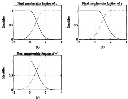
v to o _v c~ I

(15)

Y.-C. Chen, C-C. Teng / Fuzzy Sets and Systems 73 (1995) 291-312 305 Assume that for the F N N C , Pc = {e(t),~(t)}, each input variable has three fuzzy partition sets, so Rc = 3 x 3 = 9 rules. F o r F N N I , Pi = {u(t),y(t),~(t)}, each input variable has three fuzzy partition sets, so R~ = 3 x 3 × 3 = 27 rules. See Figs. 3(a) a n d (b), 4(a)-(c). E a c h cycle takes 10 s. After 18 cycles, the plant can be controlled very effectively. A test set (0.8, 1.0) is applied to the system, with a step size of 0.02 s.

In each cycle, if the value of a particular c o n s e q u e n c e link rule is smaller t h a n 1/Rc = ~ for the F N N C or

1/R~ = ~ for the F N N I , then we eliminate t h a t rule. In the final simulation result, we find that the F N N C has

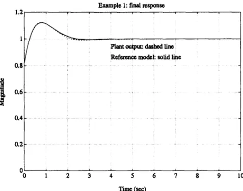
four rules a n d the F N N I has eight rules. See Figs. 3(c) a n d (d), 5(a)-(c), a n d Table 1. T h e final simulation result is s h o w n in Fig. 6.

T h e results s h o w t h a t the F N N c o n t r o l system has the ability to interpolate c o n t r o l response if an u n t r a i n e d set is closed to all trained sets.

i

Final ~ p funtion of u 0.5 ... i. . . ° ' ° i -2 0 2 4 (a)

F'mal memlmmhip funlion of y'

0.5 0 " ' ' ' " -2 0 2 4 (¢) 1 0.5 0 -2

Final membentMp funtion of y

0 2 4

Fig. 5. Final membership functions of identifier: (a) u, (b) y, (c) y'.

Table 1

Learned rule weight matrix for the FNNC

e NM ZE PM

NM 0.000 0.000 0.000

ZE - 1.001 - 0.826 2.352

(16)

306 Y.-C. Chert, C.-C. Teng / Fuzzy Sets and Systems 73 (1995) 291-312

1.2

Example 1: final response

1 0.8 0.6 0.4 0.2 / l'u t o tp t: a.a d

Refea~n~ model: solid line

. . . i .. . . i . . . i ... 2 ................... i . . . . . . . . . i ! . . . ; . . . 2 . .. .. . .. .. 2 i i i i °o t 2 ; 5

6 i

Io Time (see)

Fig. 6. Final system response for Example 1. Plant o u t p u t is indicated by the dashed line, reference model by the solid line.

Example

2 (A BIBO nonlinear plant

[13,9]). In this case the plant is described by the difference equation

y(k)

+ ua(k).

y(k +

1) = 1 + y2(k)

The reference model is described by the difference equation

yr(k +

1) = 0.6 yr(k) +

r(k),

where

r(k)

= sin(2nk/10) + sin(2rtk/25).

Assume that for the F N N C , Pc =

{e(k),Ae(k)},

each input variable has five fuzzy partition sets, so Rc = 5 x 5 = 25 rules. F o r F N N I , Pi =

{u(k),y(k)},

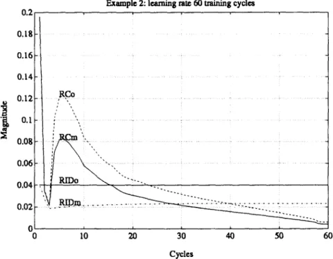
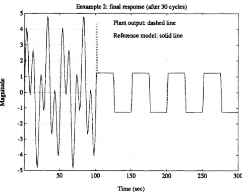
each input variable has five fuzzy partition sets, so R~ = 5 x 5 = 25 rules. See Figs. 7(a) and (b), 8(a) and (b).

Each cycle takes 100 s. Adaptive learning rates are used, starting from the initial rates of r/c ° = 0.2 and r/° = 0.04. The learning rates adapt to reduce the tracking error. The learning rates for the F N N C and F N N I are r/°, r/~', r/° and r/~', which are shown in Fig. 9. After 30 cycles this problem can be controlled very effectively. See Figs. 10 and 11. In each cycle, if the value of a particular consequence link rule is smaller than

1/Rc

-- 1/25 for the F N N C or

1/R~

= 1/25 for the F N N I , then the rule is eliminated. In the final simulation

result, we find that the F N N C has 25 rules and the F N N I has 25 rules. See Figs. 7(c) and (d), 8(c) and (d), and Tables 2, 3. The final result is shown in Fig. 11.

T o examine the adaptive ability of the model reference control structure, we repeat the simulation with the same conditions as those shown above, except that reference

r(k)

is modified as follows:

(a) After 30 cycles, the reference input is changed to

r(k)

= sin(2nk/25), see Fig. 12. (b) After 30 cycles, the reference input is changed to an impulse signal, see Fig. 13.

(17)

E' 0 Identifier p ~ o ... E' 0 Iden~ifie~ P I,k~ifier o P_ o 0 Identifier (D i 0 -n Cnnu~llet .o

i Q

~t..-

0 0 ConUoUcr P 0 ~nt~ll~ 0

~1

'~

...

i

?

Controller 0 .

(18)

308 0.2 0.18 0.16 0.14 0.12 "~ 0 . 1 - 0.08 - 0 . 0 6 - 0.04 . 0.02 - 0 0

Y.-C. Chen, C.-C. Teng / Fuzzy Sets and Systems 73 (1995) 291-312

Example 2: learning rate 60 training cycles

_ ~ R Co

I i I

10 20 30 40 50 60

Cycles

Fig. 9. Adaptive learning rates of the FNNC and FNNI during 60 training cycles.

O 1 0.9 0.8 0.7 0.6 0.5 0.4 0.3 0.2 0.1 0 0

Example 2: average error 40 training cycles

" Control error

5

Cycles

Fig. 10. Average error of the FNNC and FNNI during 40 training cycles.

(19)

Y.-C Chen, C,-C. Teng / Fuzzy Sets and Systems 73 (1995) 291-312 309 5 4 3 2 1 0 -1 -2 -3 -4 -5 t

lo

~o

Example 2: final reslmme (after 30 cycles)

• Reference ~odel: solid line

/

t ~o 50 ~ ~o 80

II

I 90 I00 Time (~.x)

Fig. 11. Final system response for Example 2. Plant output is indicated by the dashed line, reference model by the solid line.

!

5

-il

- 5 / J / J I

20 4O 60 80 100

Example 2: final r e ~ m s e (after 30 cycle 0 Plant output: d ~ l ~ l line Reference model: solid Line

Time (sex) I I 120 140

t

I I ~ I ~ 200

Fig. 12. Final system response for Example 2. Plant output is indicated by the dashed line, reference model by the solid line, tested adaptation for sinusoid signal.

(20)

310 Y.-C. Chen, C.-C. Teng / Fuzzy Sets and @stems 73 (1995) 291-312 5 4 3 2 1 0 -1 -2 -3 -4 -5

Ecxample 2: 1"real response (after 30 cycles)

t I

50 100

Plant output: dashed line Reference model: solid line

I

150 200

Time (scc)

t

250 300

Fig. 13. Final system response for Example 2. Plant output is indicated by the dashed line, reference model by the solid line, tested adaptation for impulse signal.

J

8 6 4 2 0 -2 -4 - 6 - . . . . [ -8 - - i 50 100 150

: Plant output: dashed line

. . . i . . . ~ f ~ ~ : idldUne • . . . "i ...

n

I

i I

2oo

2;0

£0

4oo Time (see)

Fig. 14. Final system response for Example 2. Plant output is indicated by the dashed line, reference model by the solid line, tested system robustness for added disturbances.

(21)

Y.-C Chen, C - C Teng / Fuzzy Sets and Systems 73 (1995) 291-312 311

Table 2

Learned rule weight matrix for the F N N C

A e ( k ) e(k) N B N S Z E P S P B N B - 3 . 2 6 6 2.135 - 1.944 2 . 6 6 4 1.445 N S 0 . 0 2 3 - 1.625 - 1.925 - 0 . 8 1 3 1.006 Z E - 1.398 - 0.971 0 . 1 8 5 - 1.545 - 0 . 0 9 2 P S - 0 . 5 3 4 - 0.521 1.011 - 1.308 0 . 3 9 5 P B - 1.956 - 1.845 - 1.126 - 1.184 - 1.658 Table 3

Learned rule weight matrix for the F N N I

u(k) y(k) N B N S Z E P S P B N B - 1.495 - 0 . 5 3 2 - 0 . 5 4 6 - 0 . 1 6 6 - 0 . 2 4 7 N S - 3.992 - 3.188 - 2.661 - 1.731 - 1.862 Z E 0 . 4 7 9 - 1.363 - 0 . 2 1 4 1.768 0 . 2 7 2 P S 2.131 1.077 2 . 4 3 7 3.615 4 . 0 8 0 P B 0 . 2 1 9 0.251 0 . 8 4 2 0.663 0 . 9 7 9

These figures show that the control structure can track the new reference model quickly. Also, the on-line adaptive ability and robustness of the model reference control structure using the F N N are acceptable.

6. Conclusion

A model reference control structure using a fuzzy neural network has been successfully applied to some difficult learning control problems. The ability of the F N N C and F N N I to learn control rules from experience and to adapt to system changes and rule degradation have been confirmed by simulation results. An approach to finding the bounds on learning rates based on a Lyapunov function was developed. The use of adaptive learning rates guarantees convergence, and the optimal learning rates were found. The FNN- based control system was tested for its on-line adaptive ability, robustness, and interpolation ability. Combining fuzzy logic and neural network computing appears to be a feasible way of dealing with real-time applications.

References

[ 1 ] C . W . Anderson, Learning to control an inverted pendulum using neural networks, IEEE Control Syst. Mag. 9 ( 3 ) ( 1 9 8 9 ) 3 1 - 3 7 .

[ 2 ] A . G . B a r t o , R.S. Sutton and C.W. Anderson, Neuronlike adaptive elements that can solve difficult learning control problems,

IEEE Trans. Syst. Man Cybern. 13 ( 1 9 8 3 ) 8 3 4 - 8 4 6 .

[ 3 ] Y . C . Chien, Adaptive fuzzy logic controller using neural networks, Master thesis, Chiao-Tung University (1992).

[ 4 ] Y . C . C h i e n , Y . C . Chert and C.C. Teng, Model reference adaptive fuzzy logic controller design using fuzzy neural network, Prec.

(22)

312 Y.-C Chert, C - C Teng / Fuzzy Sets and Systems 73 (1995) 291-312

[5] A. Guez and J. Selinsky, A trainable neuromorphic controller, J. Robotics Syst. 5(4) (1988) 363-388.

[6] S. Horikawa, T. Furuhashi, S. Okuma and Y. Uchikawa, A fuzzy controller using a neural network and its capability to learn expert's control rules, Proc. Int. Conf. Fuzzy logic and Neural Networks (Iizuka, Japan, July, 1990) 103-106.

[7] K.J. Hunt, D. Sbarbaro, R. Zbikowski and P.J. Gawthrop, Neural networks for control systems - a survey, Automatica 28(6) (1992) 1083-1112.

[8] T. Kohonon, The self-organizing map, Proc. IEEE 78(9) (1990) 1461-1480.

[9] C.C. Ku and K.Y. Lee, Diagonal recurrent neural networks for dynamic systems control, IEEE Trans. Neural Networks (1995), to appear.

[10] C.C. Lee, Intelligent control based on fuzzy logic and neural net theory, Proc. Int. Conf. Fuzzy logic and Neural Networks (lizuka, Japan, July, 1990) 759-764.

[11] Y. Li, A.K.C. Wang and F. Yang, Optimal neural network control, IFAC-INCOM (1992) 41-46.

[12] C.T. Lin and C.S.G. Lee, Neural-network-based fuzzy logic control and decision system, IEEE Trans. Computers 40(12) (1991) 1320-1336.

[13] K.S. Narendra and K. Parthasarathy, Identification and control of dynamical systems using neural networks, IEEE Trans. Neural Networks 1(1) (1990) 4-27.

[14] D.H. Nguyen and B. Widrow, Neural networks for selfqearning control systems, Internat. d. Control 54(6) (1991) 1439-1451. [15] M. Sugeno, An introductory survey of fuzzy control, Information and Sciences, 36 (1985) 59-83.

[16] M. Sugeno and T. Yasukawa, A Fuzzy-logical-based approach to qualitative modeling, IEEE Trans. Fuzzy Systems I (1) (1993) 7-31.

[17] G.J. Wang and D.K. Miu, Unsupervised adaptation neural-network control, IEEE Int. Joint Conf. Neural Networks 3 (1990) 421-428.