Optimal bit allocation for coding of video signals over ATM networks

Optimal Bit Allocation for Coding of

Video Signals over ATM Networks

Jiann-Jone Chen and David W. Lin,

Senior Member, IEEE

Abstract— We consider optimal encoding of video sequences

for ATM networks. Two cases are investigated. In one, the video units are coded independently (e.g., motion JPEG), while in the other, the coding quality of a later picture may depend on that of an earlier picture (e.g., H.26x and MPEGx). The aggregate distortion–rate relationship for the latter case exhibits a tree structure, and its solution commands a higher degree of complexity than the former. For independent coding, we develop an algorithm which employs multiple Lagrange multipliers to find the constrained bit allocation. This algorithm is optimal up to a convex-hull approximation of the distortion–rate relations in the case of CBR (constant bit-rate) transmission. It is suboptimal in the case of VBR (variable bit-rate) transmission by the use of a suboptimal transmission rate control mechanism for sim-plicity. For dependent coding, the Lagrange-multiplier approach becomes rather unwieldy, and a constrained tree search method is used. The solution is optimal for both CBR and VBR transmission if the full constrained tree is searched. Simulation results are presented which confirm the superiority in coding quality of the encoding algorithms. We also compare the coded video quality and other characteristics of VBR and CBR transmission.

Index Terms—Asynchronous transfer mode, bit allocation,

im-age coding, optimization methods, quantization, rate distortion theory.

I. INTRODUCTION

W

E consider objective optimization of video coding for ATM networks. Video coding techniques can be classified as being independent or dependent. In information-theoretic terms, independent coding refers to the situation where the distortion–rate (D–R) relation of a later video unit (a picture, a macroblock, etc.) is independent of how an earlier video unit is coded, or in other words, the distortion–rate relations of successive video units are separable, while for dependent coding, it may be dependent, or inseparable. The former includes schemes such as motion JPEG [1]–[3] and certain ways of intraframe coding of macroblocks, while the latter includes those employing motion-compensated predic-tive coding such as H.26x [4]–[6] and MPEGx [7], [5]. The purpose of our study is twofold: first, to develop efficient algorithms for both independent and dependent video coding,

Manuscript received May 15, 1996; revised September 30, 1996. This work was supported by the National Science Council of R.O.C. under Grants NSC 84-2213-E-009-107 and 85-2213-E-009-068. This paper was presented in part at the IEEE International Conferences on Image Processing, Washington, DC, October 1995, and Lausanne, Switzerland, September 1996.

The authors are with Department of Electronics Engineering and Center for Telecommunications Research, National Chiao Tung University, Hsinchu, Taiwan 300, R.O.C.

Publisher Item Identifier S 0733-8716(97)04193-0.

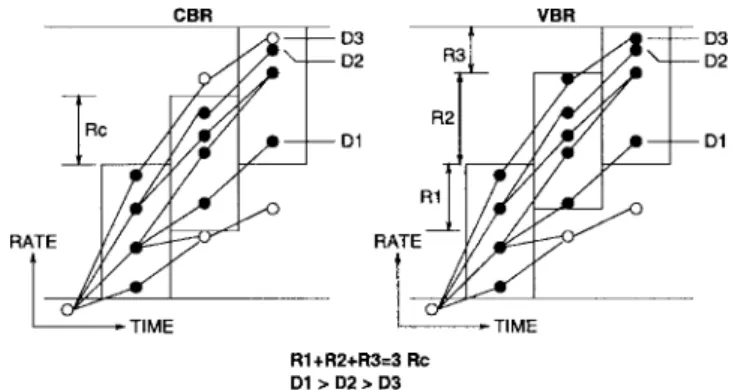
Fig. 1. Constant and variable bit-rate coding.

and second, to compare the properties of optimized CBR (constant bit-rate) and VBR (variable bit-rate) video coding.

Concerning transmission properties, it is widely held that VBR (ATM in particular) is better than CBR due to the time-varying nature in information content of typical video. A simple make-believe example may help illustrate the reason. Consider Fig. 1, which schematically illustrates the different situations one may encounter in CBR and VBR coding of the same four successive video units (numbered as, say, 0, 1, 2, and 3). Each column of dots (open or closed) under the heading CBR or VBR corresponds to a certain video unit. Each series of line segments connecting dots in different columns represents a possible way of coding through the successive video units, with the vertical position of the last dot denoting the total data rate of the coded video. ( ) are the distortions associated with three different coding paths. The upper and lower edges of each rectangle delimit the allowed total rate at each time as prescribed by the finite channel transmission capacity and codec buffer sizes. It is seen that, with CBR transmission at a constant rate , the coding path leading to a final total distortion of is not allowed because it violates the rate constraints at video unit 2. However, with VBR transmission at an average rate , it is allowed, leading to a lower total distortion, for at time 2 the transmission rate can be varied momentarily to accommodate it. It is of interest to have some quantitative comparison of VBR and CBR performance under optimized coding, which is part of our goal.

Concerning coding algorithms, Shoham and Gersho [8] proposed an optimal bit allocation algorithm for still-image coding. The algorithm does not address video coding under multiple buffer-imposed constraints, however. For independent coding, Ortega et al. [9] considered trellis search (where each 0733–8716/97$10.00  1997 IEEE

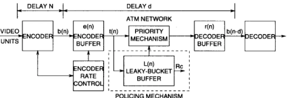
Fig. 2. Codec system with ATM network.

trellis node at stage corresponds to the buffer level grown out of a particular sequence of quantizing and coding of the signal up to video unit ) for finding the buffer-constrained optimal bit allocation. This method finds the optimal solution at a very high computational load. A closely related work is [10]. Ortega et al. [9] also presented several reduced-complexity algorithms which could yield nearly optimal results, among which are some that employ the Lagrange-multiplier technique. How-ever, these Lagrange-multiplier-based algorithms are heuristic. Nor is their optimality characterized theoretically. A different Lagrange-multiplier-based algorithm was considered in [12]. This algorithm makes use of multiple Lagrange multipliers to accommodate the multiple rate constraints. However, its theoretical basis and operational features have not been de-scribed clearly. Moreover, the above algorithms were derived largely for CBR transmission. A key result of the present paper is an algorithm (together with the underlying theory) which solves a multiple Lagrange-multiplier problem for indepen-dent video coding under the VBR environment of ATM net-works. (The VBR environment aside, the multiple-Lagrange-multiplier optimization is a theoretically much more involved problem than the one-Lagrange-multiplier optimization treated in [8] and employed in [9].) We also present some simulation results.

For dependent coding, two alternatives can be envisioned. One is to ignore the dependency in D–R relations, and to employ an independent-coding algorithm to reach a suboptimal solution. The other is to seek an optimal solution taking the D–R dependency into account. We consider the latter in this work. Since the problem is also one of constrained optimization, the Lagrange-multiplier approach can again be attempted. However, it is found to be very cumbersome to use, and the “monotonicity condition” [11] which, if valid, could lead to significant complexity reduction, is found to not always hold in our particular situation. An algorithm based on tree search is thus developed instead.

The coding and transmission system that we consider can be modeled as shown in Fig. 2. As seen, we assume a buffering and transmission delay of video units between encoder output and decoder input, where a video unit can be a picture, a macroblock, or some other grouping of picture elements. For simplicity, assume that the encoder and the decoder have infinite processing speed. The encoder performs delayed coding with delay equal to video units. With delayed coding, the encoder factors the relative complexity

of present and “future” video units into consideration in its bit allocation and is therefore more likely to yield a better coding quality than considering only one video unit at a time [13, ch. 9].

At time , the encoder outputs bits (the encoded bits for video unit ) to the encoder buffer, which outputs bits to the ATM network. The ATM network employs a leaky-bucket (LB) policing mechanism. In optimization of video coding, the finite codec buffer sizes and the ATM network policing mechanism place rate constraints on the coded video [14], [16], [17]. More specifically, the decoder buffer fullness and the ATM policing mechanism impose constraints on the allowed transmission rate at time , which affects the encoder buffer fullness, and in turn imposes constraints on the allowed encoder output rate at time . Optimization of coding must operate under these constraints. Then a specific transmission rate must be determined for each . In a sense, the optimization is a joint encoder and channel rate control problem, and we have two control targets, namely,

and .

In what follows, we first derive the rate constraints due to fi-nite channel capacity and fifi-nite codec buffer sizes in Section II. These constraints are derived for VBR transmission. But they also apply to CBR transmission in a simplified form. Section III then addresses independent coding. It formulates the optimization problem, and develops an efficient Lagrange-multiplier-based algorithm for solving the problem. Section IV discusses dependent coding, and outlines a tree-search-based solution. Section V presents some simulation results, and Section VI is the conclusion.

II. OPTIMIZATION CONSTRAINTS

We now derive the rate constraints under which the encoder has to operate. We first consider the constraints on the channel rate due to finite decoder buffer and the leaky-bucket ATM policing mechanism, and then that on the encoded bits due to the finite encoder buffer and channel rate. Then we explain how these constraints function in coding.

A. Constraints on the Transmission Bit Rate

As said, constraints on the transmission bit rate are derived from limits of the decoder buffer and the LB buffer.

We first check the rate constraints imposed by the finite decoder buffer size. Let denote the decoder buffer size, and let be the decoder buffer level after extraction of

[data for the th video unit] for decoding. Then (1) Cumulated over time, it yields

(2)

where . To avoid decoder buffer under- and overflows

at time [i.e., to ensure ,

therefore, must satisfy

(3)

The quantities and define rate boundaries

within which decoder under- and overflows, respectively, are avoided. The factor will be explained later. Equation (3) summarizes the constraints on transmission rates from the limited decoder buffer size (as well as from the bits of previously encoded video units) up to time . In writing the

inequality, we have assumed and to be given.

We now move to check the constraints from the network policing function. Let denote the LB size, the LB fullness, and the average leak rate. Then

(4) Cumulating over time, we obtain

(5)

where . To ensure that the policing mechanism passes all data intact, must be such that the LB never overflows, i.e., [14]. To fully utilize the channel capacity, we would desire to avoid LB underflows as well, i.e., to let . In this case, the cumulated channel rates are constrained by

(6) where and the role of will be explained later.

and specify boundary conditions for absence of LB underflow and overflow, respectively.

Equations (3) and (6) together give the constraints on the transmission rate at any time after . They depend on the buffer sizes, current buffer fullness, as well as the rates of some previously encoded video units.

Fig. 3. Typical region of permitted rates when coding delay= 1 video unit.

B. Constraints on the Encoded Bits

We now derive constraints on encoded bits due to the transmission rate and the finite encoder buffer size. Let denote the encoder buffer size, and let be the encoder buffer level after the th picture has been coded. With

and as defined earlier, we have

(7) Cumulated over time, it yields

(8) where . To avoid encoder buffer under- and overflow at

time , we need and thus

(9) which constrains the cumulated number of encoded bits at all future time under a given sequence of transmission rates

.

The scale factor is introduced in (3), (6), and (9) for the purpose of rate control, so that a target buffer fullness less than

and can be set for (the conclusion of the delay-coded video units); that is, for and for . For example, we may choose to be less than, equal to, or greater than at according to whether the video units after are expected to be more complex, equal in complexity, or less complex than the video units

that are being delay encoded.

The constraints (9), with given , mark out a region of permissible values for the vector

in the -dimensional space. For example, for a

typical region may look like the shaded area shown in Fig. 3. For signals with convex D–R relations, the optimal solution should situate on or near the top border of the region. C. Interpretation of the Rate Constraints

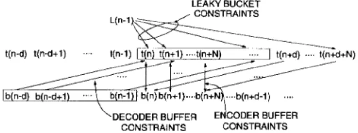
Fig. 4 summarizes the relation among constraints (3), (6), and (9) at time , when we begin the encoding of video units . For convenience, we draw the case for . At time , the encoded bits and the LB fullness are available for time up to . (They are already fixed and cannot be

Fig. 4. Relation among rate constraints.

changed.) The bits and

place constraints on

and the constraints are unidirectional. The relation between

and is different. The situation

can be appreciated by looking at Fig. 2. While the allowed

transmission rates [as determined

from (3) and (6)] constrain as

in (9), after the encoding of video units (which

determines ), specific values for

must be determined to facilitate

transmission. For this, now act as

constraints through the finite encoder buffer size. From this perspective, (9) can be rewritten into

(10)

where and and specify boundaries

be-yond which encoder buffer over- and underflow, respectively, would occur. Therefore, the constraining relationship between

and

is bidirectional, with both directions at work at different times during the coding and transmission process. Moreover,

and

are related through the decoder buffer relationship (2). Hence, the former are constrained by the latter in the following way:

(11)

for (a reformulation of (3) for these values

of ). The constraints are again unidirectional for the coding of video units . (They will work in the other direction in the coding of later video units.)

In summary, in coding video units , the effective

constraints are (3) for , (6) for ,

(9) and (10) for , and (11) for .

Under constraint are quantities, namely,

and .

III. OPTIMAL INDEPENDENTCODING—THE LAGRANGE MULTIPLIER APPROACH

We now consider optimal coding in the case where the video units are independently coded, examples being motion JPEG and certain ways of intraframe coding. Consider an additive distortion measure, that is, the encoder seeks to conduct the following minimization:

(12)

where denotes all possible ways of coding video unit and denotes the corresponding distortion in this video

unit, subject to the constraints on in

(9) together with (3) and (6). The choice for is limitless, of which the MSE and the weighted MSE are two common examples.

As discussed, we approach this problem by way of Lagrange-multiplier optimization. The Lagrange-multiplier method only finds solutions on the convex hull of a D–R relation, while it is known that actual D–R relations for real video may be nonconvex. Hence, it is possible that the Lagrange-multiplier solution is suboptimal, and the truly optimal solution lies somewhere between it and the rate-region boundary. A search procedure can be appended to the Lagrange-multiplier method to look for the truly optimal solution [8], but it is deemed too complicated to implement and may lead to small improvement only.

A. Suboptimal Control of the Transmission Rate

For the present work, it appears overwhelming to consider all possible bit allocations afforded by the rate constraints derived in the last section (and illustrated in Fig. 4) in the Lagrange-multiplier optimization. We take a handwaving mea-sure, and employ a kind of greedy method to control the transmission rate , but leave under the full freedom of the constraints that remain. More specifically, the rates are controlled in the following way.

Intuitively, we should maximize in hope of

the best video quality. From (9), this calls for choosing

the maximum possible value for for then, the

allowed range for is the highest among all

possible. From (3) and (6), should not exceed

. Thus, the rate budget for is set to be

(13)

[where for notational convenience we write as

a shorthand for ] and the allocated total rate

should be as close to the right-hand side (RHS) as possible. In determining the bit allocation for the video subsequence

(where ), we allow to be as large as

possible to avoid encoder buffer overflow or to be as small as possible to avoid encoder buffer underflow up to , without regard for how this would affect later coding. (Step S3 in the algorithm presented later in this section is an enbodiment of

this principle.) After encoding of video units , we

determine according to

(14)

where . Results from several specific choices

of are presented later.

The above method of rate control is acknowledgeably suboptimal. We leave fully optimal solutions to potential future work. (We remark that this is an issue only for VBR transmission. For CBR transmission, the channel rate is fixed, and there is no issue of suboptimality.)

B. Lagrange-Multiplier Optimization

With greedy determination of , only are subject to optimization. Applying the Lagrange-multiplier technique to (12), we obtain

(15)

where are the Lagrange-multipliers. Term

a Lagrange-multiplier vector. To find the optimal solution, we will have to step through a series of candidate Lagrange-multiplier vectors. For each given vector, the above minimum can be evaluated if we have the D–R relation for video units to . Therefore, the first task in Lagrange-multiplier optimization is “data generation” (using the term of Ramchandran et al. [11]) which computes the D–R relation for each macroblock in video units to . Next, we have to find the optimal Lagrange-multiplier vector.

Optimization under multiple constraints (hence multiple Lagrange multipliers) can be very difficult unless the problem possesses some simplifying structure. Fortunately, we have such a situation: the multimultiplier problem (15) can be broken down into a series of one-multiplier problems, each of which is readily solvable using the technique of [8]. The derivation of this result takes some theoretical excursion, and is relegated to the Appendix. Below, we describe the ensuing algorithm. It has a recursive construct.

First, we freeze all Lagrange multipliers except to zero and solve (15) subject to the constraint (13) on the total rate. This is a one-Lagrange-multiplier problem which is readily solvable using the method of [8]. The solution will satisfy the total-rate constraint for video units but not necessarily at any time between and . In the case , for example, the solution may lie along the line that defines the top border of the allowed rate region in Fig. 3, such as point A, assuming the D–R relations are convex. We thus have to check for possible violation of the “nonterminal” rate constraints. If the constraints are satisfied everywhere, then we have obtained the optimal bit allocation. Otherwise, some

Fig. 5. Concept of anchor points. Abscissa denotes time (index of video units). Ordinate positions of circles give cumulated bit allocation for video units[n 0 N; m]. For simplicity, the upper and lower bounds on cumulated rate are drawn as straight lines. This is the case for CBR transmission. For VBR transmission, they may be jagged.

other solution has to be found. For the example above, the true solution should lie in the upper right corner of the allowed rate region.

To obtain the true solution, we first identify the anchor point in video sequence , defined as the last video unit that violates the RHS (overflow) constraint in (9) that comes before the first violation of the left-hand side (LHS) (underflow) constraint, or the last video unit that violates the LHS constraint in (9) that comes before the first violation of the RHS constraint, whichever condition holds. If only one kind of violation occurs over the sequence, then it is the last video unit before where violation occurs. The idea of anchor points is illustrated in Fig. 5. Denote the anchor point by . Define the video subsequence as the anchor subsequence. Now, we can modify the bit allocation to address the violations.

The basic idea is as follows. Conduct an optimal bit alloca-tion for the anchor subsequence subject only to the total-rate constraint on this subsequence (a one-Lagrange-multiplier optimization problem). Examine whether all of the nonterminal rate constraints for are satisfied. If not, then identify the anchor point in in the same manner as we have done for the overall sequence , set to denote this new anchor point, and recursively descend into the new anchor subsequence as we have done in the case of the initial anchor subsequence above. If yes, then we have obtained the optimal bit allocation for . For “sliding-window coding” in

which video units are merely employed for

bit allocation but only video unit is actually encoded and sent to buffer at each time , we may stop here. For “jumping-window coding” with jump distance , in which

all video units are actually encoded at time

and buffered for later transmission, we continue with the following: subtract from the rate allocated to the last anchor subsequence, advance to the subsequence and repeat the above procedure to allocate the remaining bits to it.

To effect the one-constraint optimal bit allocation over an anchor subsequence, we freeze all Lagrange multipliers except

to zero, and conduct the minimization of (15) subject to the constraint (9) for only, with the additional requirement that the solution should lie on or near the LHS or the RHS rate boundary at depending on which boundary is exceeded at the anchor point. We remark that, due to the recursive nature of the overall procedure, the whole

delay-encoded video sequence can be viewed as

the startup anchor subsequence.

As an example, consider again the example shown in Fig. 3 where the initial optimization subject only to (13) yields a solution at point A. The anchor point is thus and the anchor subsequence is . Optimized coding of the anchor subsequence subject to the RHS of (9) for would yield a solution along the right border of the rate region. The desired “corner solution” is obtained by allocating the remaining bits to and optimizing its coding subject to this rate constraint.

We summarize the foregoing Lagrange-multiplier optimiza-tion procedure into an algorithmic descripoptimiza-tion.

Algorithm 1: S1: Compute constraints on the total bit

budget for the video units using (13). Set

violation overflow, and .

S2 (Trial optimization): Employ a Lagrange multiplier to perform the optimization

subject to

if violation overflow

if violation underflow (16)

(where the inequalities should be satisfied as close to being equality as possible). Obtain the associated bit allocation

.

S3: Check (9), (3), and (6) for any buffer under- or overflows under the above bit allocation. In their absence, go to S4. Otherwise, locate the anchor point in as defined previously. Set the variable violation to indicate the kind of violation. Set bit budget

if overflow

underflow

for video units . Set and go to S2.

S4: Determine according to (14),

and update the buffer levels and using

(1), (4), and (7).

If ( ) go to S5; else let ,

and and go to S2.

S5: Output and for . Increment

by and go to S1.

The above algorithm applies to jumping-window coding with jump distance . Modification of it for sliding-window coding is easy and omitted.

C. Complexity Analysis

The above algorithm contains two phases: a data generation phase and a Lagrange-multiplier optimization phase. Assume that in the data generation phase, we obtain the D–R relation of each video unit in . In addition, the “singular Lagrange multiplier values” [8] for these video units are also obtained and sorted. (A singular Lagrange multiplier for video unit is a number for which there is more than one solution

to the problem , i.e., more than one way

of quantizing the video unit to yield the minimum. It is equal to the slope of a line segment on the convex hull of the D–R relation of the video unit.)

For the Lagrange-multiplier optimization, assume there are singular Lagrange multipliers per video unit. is upper bounded by the product of the number of macroblocks in each video unit and the number of selectable quantizers for each macroblock. In the above-presented algorithm, the most computation-intensive step is S2 (trial optimization). In comparison, other steps have negligible complexity. Consider first a worst case scenario where the trial optimization always results in constraint violations (except when ), and the new anchor point always occurs at . It then takes trial optimizations on anchor subsequences of lengths , respectively, to obtain optimal bit allocation for the video unit . For sliding-window coding, this is when we slide the window and begin optimization for the next segment of video. For jumping-window coding, we

continue optimization for video units , which

requires trial optimizations to attain the optimal solution

for video unit , and so on.

A pass over S2 requires, at worst, search among

singular Lagrange multipliers for solution, at a

complex-ity on the order of steps employing

logarithmic search. Each search step requires up to the order

of arithmetic operations to compute the total

rate and compare it against the constraint. For sliding-window coding, therefore, the worst case complexity [denoting it by

] is on the order of

(17) per video unit. This worst case scenario may appear too pessimistic. However, we have too few data to define a statis-tically meaningful majority or average situation. Nevertheless, it seems heuristically reasonable to consider the following

more favorable situation than the worst case, namely, that the anchor subsequence reduces geometrically in length with each recursion. We can derive (derivation omitted) that the complexity in this case, denoted , is an order of

magnitude lower in power of than as

(18) per video unit, where is the factor by which the lengths of anchor subsequences reduce in each recursion.

For jumping-window coding, the worst case complexity is given by

(19)

for the whole sequence . Dividing it by , we

obtain the average complexity per video unit, which is the same in order of magnitude as except for a three-times lower proportionality constant. For the more favorable situation of geometrical shrinkage of anchor subsequence, a bound on complexity is given by

(20)

for the whole sequence or of it per video

unit. If, in addition, we assume that the final set of anchor subsequences for which the optimal solutions of S2 satisfy all rate constraints is also geometrically distributed in length, then the complexity for jumping-window coding is brought down further by one order of magnitude in power of to

(21) where is a constant, for the whole sequence and thereof per video unit—which is lower by an order of magnitude in power of than sliding-window coding.

Work is in progress concerning an algorithm which guar-antees geometrical convergence regardless of how anchor subsequences shrink in recursion [15].

IV. OPTIMAL DEPENDENT CODING—CONSTRAINED TREESEARCH

We now direct attention to optimal bit allocation for coding schemes where the D–R relation of a later video unit may depend on how an earlier unit is encoded. Examples of such schemes include ITU-T’s H.26x series recommendations and ISO’s MPEGx standards.

In common video coding schemes, the distortion and rate of a video unit are both controlled by choice of the quantizer step size. In the case of dependent coding, different choices of the quantizer for an earlier video unit may lead to different D–R relations for later video units. Hence, the collection of all possible coding choices for a video sequence, say

, can be organized into a tree. The first-level nodes are defined by the quantizer choices for unit . Each node has as many children (second-level nodes) as there are choices for the quantizer. Each tree branch is associated with a certain distortion and a certain data rate. In the case of independent coding, the tree degenerates into a trellis because successive levels’ distortion–rate relations are independent. Such a trellis is employed in solving for the constrained optimal bit allocation in independent video coding in [9] and [10]. Use of the tree in dependent coding is considered in [11], where the tree is also termed a trellis.

Several methods exist for finding the optimal solution. One is still using a Lagrange multiplier approach. But since the D–R relations of successive video units are not separable, performance of the minimization (15) for a given set of Lagrange multiplier values can no longer be accomplished by minimizing for each video unit individually and then combining the results, but entails a search over all of the terminal nodes of the above D–R tree for the lowest value of distortion rate . Aside from the issue of tree search under given multiplier values, another issue is the number of multiplier values that need be searched to find a solution at the desired constraint boundary. This number can be mini-mized using a logarithmic-type search scheme, such as the hierarchical method in [16].

To reduce the tree-search complexity for given Lagrange multiplier values, a kind of “monotonicity condition” in the D–R relations of successive video units was assumed and exploited in [11]. Briefly, this condition says that a video unit will have a worse D–R relation if its preceeding video unit is quantized with a coarser step size than if with a finer step size, in the sense that the D–R relation of the latter lies toward the upper right of that of the former. While this is experimentally confirmed in some cases [11], we have found that the condition may not always hold for any conceived way of coding under the H.26x or the MPEGx framework. Some examples are shown in Fig. 6. The figure plots the operational D–R relation of the second picture in two successive predictive-coded pictures under H.261 framework. and denote the average quantizer step sizes used in the encoding of the previous and the present pictures, respectively. Under H.261, there are many ways to encode a picture to yield the same average quantizer stepsize. Points in the figure correspond to that minimizing the distortion in the respective pictures. Note that a segment of the curve for clearly lies to the lower left of the curve for , violating monotonicity.

The above violation of monotonicity can probably be at-tributed in part to the fact that, in “optimizing” the quantization vector, we only minimized the distortion, but paid no attention to its rate implications. But this is at least one reasonable (although suboptimal) way to trim the full coding tree for delayed coding over a window of several pictures—the tree size could be astronomical without trimming. (Alternatively, one could conceive of the existence of a problem whose solution set observes the structure of this trimmed tree. In this case, the problem is endowed with inherent nonmonotonicity.) Another possible cause of nonmonotonicity, under H.261 and similar coding frameworks, is the allowed use of intraframe

Fig. 6. Example showing that monotonicity may not always hold. coding for macroblocks in a predictively coded picture. If the reference picture is coarsely quantized, the encoder may choose to use intraframe coding for the present picture, which may result in a lower distortion at the expense of more bits for the present picture when compared to the case where the reference picture is more finely quantized. This already could result in violation of the monotonicity condition. Adding to it is that the variation in rate and distortion from the above phenomenon could be irregular to sum up to more conspicuous violations.

Nevertheless, one should note that the above in no way nullifies the usefulness of the monotonicity assumption in reduction of complexity for tree/trellis search. The reduced-complexity algorithm so obtained can be applied even in the face of nonmonotonicity to arrive at a suboptimal solution. However, in the present work, we opt to avoid this addi-tional source of potential suboptimality. In this case, with the dependency in D–R relations and without the monotonicity condition, the Lagrange multiplier method appears too tedious and inefficient. (The Appendix touches on this briefly.) An attempt was made to simplify the problem by disregarding some constraints in (3), (6), and (9), in particular, those restricting encoder buffer underflows. Simulation results show that this, in many cases, increases the distortion in the coded video because these underflows do occur, and the ensued bit stuffing nibbles away channel bandwidth that could otherwise be used for video data, although the increase in distortion may not always be significant.

In conclusion, we deemed the Lagrange multiplier ap-proach too unwieldy in dependent coding, and we opted for straightforward search over the coding tree under the previously derived rate constraints. The search can be carried out recursively by growing the tree one level at a time (corresponding to quantization and coding of one successive video unit using all possible quantizer step sizes), trimming the new-grown branches according to the previously derived rate constraints, and recording the distortion associated with each survivor path, until we come to the end of the video

(a)

(b)

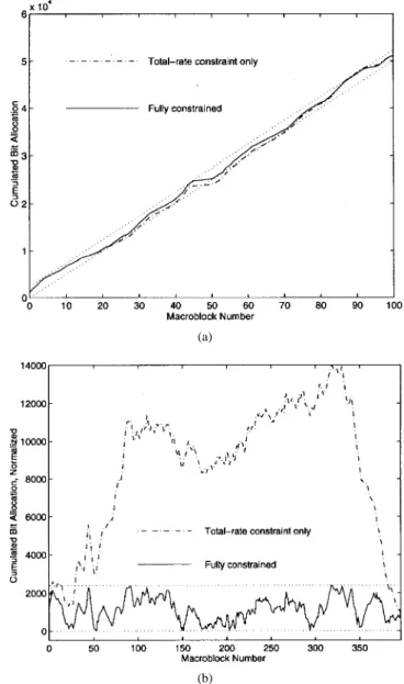
Fig. 7. Bit allocation under optimal independent encoding. Straight lines in each plot mark the upper and lower constraints on cumulated rate at each time. (a) Case of 100 macroblocks. (b) Case of 396 macroblocks. For clarity, curves for (b) are “flattened” by subtracting500n from the cumulated rate at macroblock n; thus, we have the term “normalized.” As a result, the rate constraints actually correspond to encoder buffer boundaries, and the normalized cumulated rates correspond to would-be encoder buffer levels should the buffer be able to accommodate the coded bits.

units under delay encoding. The survivor path with minimum total distortion then gives the solution. With full-tree search, the solution is optimal under either CBR or VBR transmission [9].

The sliding-window video sequence coding procedure can be described as follows. Modification to jumping-window coding is straightforward.

Algorithm 2: S1: Grow the coding tree recursively, one level at a time, subject to the rate constraints derived earlier.

S2: Find the path with the least total distortion. Quantize and encode video unit using the quantizer step size in the optimal solution. Determine the transmission rate subject to (14).

S3: Update the buffer levels , and .

Fig. 8. Variation of optimal Lagrange multipliers with time.

V. A SIMULATION STUDY

We simulate both independent and dependent coding. The goals are, first, to examine the performance and properties of the (sub)optimal coding of earlier sections, and second, to compare the performance of CBR- and ATM-type VBR transmission. The codec and transmission delay is set equal to (the delay-encoding “window size”) in all cases. For convenience, we use PSNR to measure coding performance, although it may not be a subjectively meaningful measure at all times.

A. Independent Coding

We consider H.261-type intraframe video coding, and let each video unit be a macroblock. The encoder buffer size is set to be 2400 bits, and the channel rate per video unit is 500 bits. We employ jumping-window encoding. The first picture in the well-known salesman sequence, in CIF format (396 macroblocks), is encoded.

We first inspect the variation in video rate from

opti-mized bit allocation. For this, we let and

en-code the first 100 macroblocks of the picture under CBR transmission. The result is plotted in Fig. 7(a). For compar-ison, the result from optimization only under the total-rate constraint (but not buffer constraints at any earlier time) is also shown. Observe in Fig. 7(a) that, for video units near 20–30 and 45–60, where the buffer constraints are vi-olated in the total-rate-constrained solution, the fully con-strained optimal bit allocation is sometimes close to the constraint boundary, as one might expect from the discussions in the Appendix. It is also of interest to observe that the two curves show similar variations over these regions. The rate variation from fully constrained and total-rate-constrained optimization of all 396 macroblocks together is shown in Fig. 7(b).

We next compare the performance and characteristics of CBR and VBR transmission. The LB size and leak rate are set to be 4800 and 500 bits per video unit, respectively. The

(a)

(b)

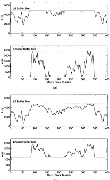
Fig. 9. LB and encoder buffer fullness under different transmission rate control schemes. (a) High transmission rate. (b) Medium transmission rate.

initial and target LB levels are both set to be half full so that the total bits available for coding are the same under CBR and VBR. Results in Fig. 8 show that VBR offers a slightly higher average PSNR. The difference is small, presumably due to the video material in addition to the use of a suboptimal transmission rate control scheme. We expect a more significant difference in performance for material showing greater variation in complexity across video units. (Indeed, it will be seen later in dependent coding results that VBR yields a prominent gain at scene cuts.) Curves in Fig. 8 also show that, compared to CBR, the Lagrange multipliers under VBR transmission exhibit less variation, and are closer to the total-rate-constrained solution, which implies a smaller deviation of bit numbers from the total-rate-constrained solu-tion, and thus a better match of transmission rate with video complexity.

Reconsider the determination of transmission rates under VBR transmission. Equation (14) practically specifies an in-finitude of possible choices. Specifically, we may take the

Fig. 10. Encoded and transmitted bit rates. Top: high transmission rate; bottom: medium transmission rate.

weighted sum of the upper and the lower bounds as

(22)

for , where and .

Fig. 9(a) is obtained with . We see that, in

this situation, the encoder buffer is often empty when the LB is not full, which indicates that the LB, or more exactly, the ATM network, is absorbing the variation in the video rate for a best

coding quality. Fig. 9(b) is obtained with ,

which has led to a half-full encoder buffer when the LB buffer level is not high. As further illustration, the encoded and transmitted bit rates in each case are depicted in Fig. 10, which shows that the transmission rate follows the encoded bit rate when the LB is not full and is kept at the leak rate when it is full. Interestingly, the two transmission rate control methods have resulted in the same received video quality because of the same solution in bit allocation.

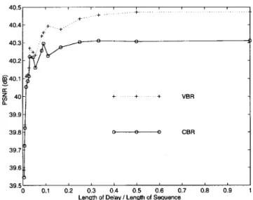
We now examine the variation in coding performance as a function of the length of encoding delay. Fig. 11 shows the PSNR results obtained with different coding delays for both CBR and VBR transmission. The best performance occurs at full-length delay. But it is interesting that the PSNR is not monotonically increasing with delay for either CBR or VBR, which can be expected since the forced satisfaction of for a block of video units may not be optimal over a longer or shorter block. But the suboptimality should lessen as long-enough blocks are used. For VBR transmission, the PSNR improvement over CBR transmission increases as increases. B. Dependent Coding

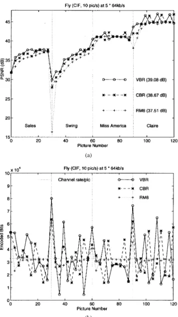
We consider H.261-type coding. Fig. 12 shows the average PSNR results obtained from (sub)optimal CBR and VBR coding of the CIF Salesman sequence at 10 pictures/s at different (average) rates, where the suboptimality arises due to the use of distortion-minimized average quantizer step sizes

Fig. 11. PSNR performance at different encoding delays (in fractions of total sequence length, i.e., 396 macroblocks).

Fig. 12. Overall PSNR of RM8 and delayed coding of CIF Salesman sequence at 10 pictures/s atp 2 64 kbits/s.

for each picture for simplicity. These average quantizer step sizes are limited to between 2 and 36, in steps of two. For comparison, results from the widely used reference algorithm RM8 [18] is also included. For fairness in comparison, for all algorithms, the first picture in the sequence is coded the same as in RM8. The codec buffer sizes are

where is as defined in the figure, and the codec delay is two pictures. For VBR transmission, the LB begins (somewhat unfairly) at empty at the second picture. It is seen that the suboptimal CBR coding yields approximately 1.0 dB gain over RM8, and the suboptimal VBR coding gains roughly an additional 0.2 dB over all rates. Fig. 13 shows the variation of per-picture PSNR at an average rate of 384 kbits/s ( ).

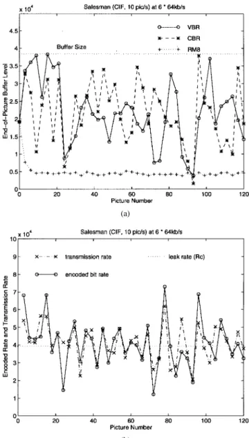
It is of interest to examine the buffer-level variations in the different coding methods. Fig. 14(a) plots the encoder buffer level at the end of each picture for each method. Fig. 14(b) further shows the number of encoded bits and the VBR channel transmission rate. Observe from Fig. 14(a) that the buffer-level variations in the delayed-coding solutions are greater

Fig. 13. PSNR of RM8 and delayed coding of CIF Salesman sequence at 10 pictures/s at 384 kbits/s.

than that in RM8. On the positive side, this may be due to the fact that the delayed-coding solution makes better use of the buffer space to catch the complexity variation in successive pictures and adjust the bit rate accordingly. However, there are at least two other possibilities. And it is possible that all of these forces are at work at the same time to different degrees. First, as noted above, for simplicity, we have limited the set of quantizer step sizes, or equivalently, the number of tree nodes at each level. This may have affected the algorithm’s ability to find smoothly varying bit allocations for successive pictures. Second, in delayed encoding, if somehow a picture is allocated a high rate, then later pictures may be encoded to a high fidelity more easily (because of a good reference picture in predictive coding), but they also are subject to more stringent rate constraints. Over time, the quality may suffer until a point where the high complexity in a picture (due to a poor reference in motion-compensated prediction) and the gradually released rate constraints again lead to a high-rate coding. The end result may be oscillating rates, PSNR, and buffer levels as shown in Figs. 13 and 14. In VBR coding, where we have an additional degree of freedom in controlling the transmission resource, the above could be further enhanced. However, we should note that oscillation in PSNR, by itself, may not be an undesirable phenomenon since the aim in delayed coding is to achieve minimum total distortion over several pictures rather than homogeneous PSNR.

Heuristically, the performance improvement due to delayed coding should be especially acute at a scene cut. This is because of the -picture worth of “foreknowledge” provided following the scene cut, while RM8, by its simple feedback control of the quantizer step sizes, does not make use of this foreknowledge, even if available. To verify this point, we consider a composite sequence made up of 30 pictures each of Salesman, Swing, Miss America, and Claire in that order. The composite sequence is named Fly, in which the several scene changes can be used to verify the effectiveness of the delayed-coding schemes in bit allocation and the flexibility offered by VBR ATM rate control.

(a)

(b)

Fig. 14. Variation in buffer level and rate in RM8 and delayed coding of the Salesman sequence. (a) Buffer level variation. (b) Encoded bits and channel transmission rate in VBR coding.

Fig. 15(a) shows the PSNR result from coding Fly at 320 kbits/s. We see that the delayed coding schemes can have a significant advantage immediately following a scene cut, possibly at the expense of a somewhat lower performance immediately preceding it. The PSNR performance of VBR ATM transmission is significantly better than that of CBR at scene changes (although the edge in sequence-wise average PSNR is less significant). And we see from Fig. 15(b) that the VBR ATM transmission, by its greater flexibility in rate control, allocates more bits than CBR or RM8 to the picture after a scene cut.

VI. CONCLUSION

We considered objective optimal encoding of video se-quences for ATM networks. Both independent and dependent coding were investigated. They can be formulated as opti-mization problems subject to multiple rate constraints arising from the finite channel transmission rate and the finite codec

(a)

(b)

Fig. 15. Coding of the CIF Fly sequence by RM8 and delayed coding at 10 pictures/s at 320 kbits/s. (a) PSNR performance. (b) Bits per picture.

buffer sizes. For independent coding, we derived an efficient bit allocation algorithm based on the use of multiple Lagrange multipliers. In this algorithm, we exploited the monotonic relation between total distortion and the amount of deviation from the constraint boundaries. The algorithm is optimal up to a convex-hull approximation of the D–R relations in the case of CBR transmission. It is suboptimal in the case of VBR transmission due to the use of a suboptimal transmission rate control method. For dependent coding, the aggregate D–R relationship exhibits a tree structure, and the Lagrange multiplier approach becomes rather unwieldy. We resorted to a constrained tree search approach. The solution is optimal for both CBR and VBR transmission if the full constrained tree is searched.

We presented some simulation results which confirm the superiority of the coding quality of the derived encoding algorithms over simpler schemes such as RM8. In addition, (sub)optimal coding under VBR transmission, as expected, has yielded higher PSNR performance than that under CBR

trans-Fig. 16. Nonoptimality with unequal Lagrange multipliers.

mission, although the difference appears not very significant except at scene cuts.

The ability of the optimization approach to efficiently al-locate bits among pictures with differing complexity could be further exploited for bandwidth allocation and coding of multiple video sources for transmission over a shared channel.

APPENDIX

THEORY OF THELAGRANGE-MULTIPLIERCODINGALGORITHM For simplicity, consider only convex D–R relations. Define

, . Then (15) can be

rewritten as

(23)

where the equality holds due to the independence in the D–R relations. Since there is a one-to-one correspondence

between and , characterization of can be

accomplished by characterizing . For convenience,

term the prime Lagrange multipliers. Now,

as-sume tentatively that the D–R relations associated with the video units are continuous. And assume that the optimal bit allocation touches one of the two boundaries in (9) at time , where . In particular, it touches the RHS boundary at so that the bit budget is fully

consumed. Further, let . Then we have the

following.

Lemma 1: The optimal bit allocation is such that , , are constant over each video subsequence

.

Proof: Suppose, in the optimal solution,

for some . Then in minimization of

for we have the situation

in Fig. 16 where and are the optimal solutions. Due to the different slopes in the D–R curves at and , we can reduce the total distortion without changing the total rate by

moving bits from to until either or until a

constraint in (9) is reached somewhere in . The former contradicts the optimality assumption of the original solution, while the latter contradicts the assumption that the boundaries in (9) are not touched in .

Define the optimal anchor point as the last video unit before which the optimal prime Lagrange multipliers are equal,

i.e., . And call the subsequence

the optimal anchor subsequence. We now prove that the anchor point in each recursion of the algorithm described in Section III will be located at or after the optimal anchor point. The proof consists of two steps. First, we show that the anchor point obtained from the initial optimization (yielding optimal ) is located at or after the optimal anchor point . Then we show that the anchor point will stay at or after the optimal anchor point with each recursion in the algorithm.

Lemma 2: The initial anchor point obtained by optimiza-tion subject only to the total rate constraint is such that

.

Proof: We showed earlier that the sequence of optimal prime Lagrange multipliers is piecewise constant with

magnitude changes occurring only at some .

Four cases can be envisioned: 1) wherever

( ), the boundary in (9) that is touched at is

the RHS boundary; 2) the RHS boundary in (9) is touched at and there exists some time where the LHS boundary is touched and ; 3) same as 1), but replace the RHS by the LHS; and 4) same as 2), but replace the RHS by the LHS and vice versa. We address the first two cases only since the other two are complementary.

For case 1), we show that and ,

and the conclusion follows. To show that , assume . Then we have the situation of Fig. 16, with and in the roles of and , respectively. Bits can be moved from video unit to to reduce distortion while keeping the same total rate. But then the total rate at would shift inside the RHS boundary in (9), contradicting the assumption that the optimal solution touches that boundary

there. To show that , assume . Then since

is nondecreasing in and .

By convexity of the D–R relations, the total rate obtained under would be lower than in the optimal allocation, contradicting the assumption that satisfies the total rate constraint. Therefore, . By convexity in the D–R relations, bits allocated to video units under are more than that under . Hence, there is overflow at and no underflow before it, and thus .

For case 2), we can show that . Then if ,

there is no overflow up to and there is underflow afterwards; if , then there is overflow at and no underflow before it. The proof relies on D–R convexity as in case 1). In either case, .

Lemma 3: The anchor point will stay at or after the optimal anchor point with each recursion in the algorithm.

Proof: Consider the two cases addressed in the proof of the last lemma. For case 1), we begin the recursion by having overflow at some anchor which resulted from optimization with some Lagrange multiplier geared to satisfy a rate constraint at some “future” video unit . Optimization of coding for video units subject only to the RHS constraint of (9) at video unit by using a Lagrange multiplier will lead to a solution characterized by some

in case and in case . The proof

involves an examination of the convexity in D–R relations and the nondecreasing nature of as in the last lemma; details are omitted. Now, if , then we have obtained the optimal anchor point at together with the optimal coding of ; and we can proceed to the optimal coding of . If , then we are in a similar situation as in the proof for case 1) in the last lemma where we had , and thus a similar conclusion holds. For case 2), we begin with either an underflow at or an overflow at . In case of underflow, optimal coding of

subject to the LHS constraint in (9) at either will result in an overflow at with no underflow before it, or will result in an underflow at a later video unit with no overflow before that video unit. The proof again involves a look into the D–R convexity. In case of overflow, the situation is similar either to the immediately preceding underflow case or to case 1) discussed above, depending on where is located.

Lemmas 2 and 3 together establish the convergence of the Lagrange-multiplier algorithm toward the optimal solution in independence coding for continuous D–R relations. The discussion can be extended to handle discrete D–R relations [15].

The situation with dependent coding is much more compli-cated because the optimization objective (15) can no longer be decomposed as in the RHS of (23). For example, in the case depicted in Fig. 3 with the initial optimal solution under located at , the anchor subsequence cannot be optimized independently of . In other words, the Lagrange multiplier cannot be optimized independently of . The algorithm in Section III can be modified to accommodate this dependence, but the resulting computation can become overwhelming.

ACKNOWLEDGMENT

The authors would like to thank the reviewers for their comments which helped improve the paper.

REFERENCES

[1] W. B. Pennebaker and J. L. Mitchell, JPEG Still Image Data Compres-sion Standard. New York: Van Nostrand Reinhold, 1993.

[2] J.-J. Chen and H.-M. Hang, “A transform video coder source model and its application,” in Proc. IEEE Int. Conf. Image Processing, vol. II, Nov. 1994, pp. 967–971.

[3] Y. Takishima, M. Wada, and H. Murakami, “An analysis of optimal frame rate in low bit rate video coding,” IEICE Trans. Commun., vol. E76-B, pp. 1389–1397, Nov. 1993.

[4] Video Codec for Audiovisual Services at P2 64 kbit/s, ITU-T Recom-mendation H.261.

[5] Information Technology—Generic Coding of Moving Pictures and As-sociated Audio: Video, ISO/IEC 13818-2 and ITU-T Recommendation H.262.

[6] Video Coding for Low Bitrate Communication, Draft ITU-T Recommen-dation H.263, Oct. 1995.

[7] Coding of Moving Pictures and Associated Audio—for Digital Storage Media at Up to About 1.5 Mbit/s—Part 2: Video, ISO/IEC 11172-2. [8] Y. Shoham and A. Gersho, “Efficient bit allocation for an arbitrary set

of quantizers,” IEEE Trans. Acoust., Speech, Signal Processing, vol. 36, pp. 1445–1453, Sept. 1988.

[9] A. Ortega, K. Ramchandran, and M. Vetterli, “Optimal trellis-based buffered compression and fast approximation,” IEEE Trans. Image Processing, vol. 3, pp. 26–40, Jan. 1994.

[10] C.-Y. Hsu, A. Ortega, and A. R. Reibman, “Joint selection of source and channel rate for VBR video transmission under ATM policing constraints,” this issue, pp. 1016–1028.

[11] K. Ramchandran, A. Ortega, and M. Vetterli, “Bit allocation for depen-dent quantization with applications to multi-resolution and MPEG video coders,” IEEE Trans. Image Processing, vol. 3, pp. 533–545, Sept. 1994. [12] D. W. Lin, M.-H. Wang, and J.-J. Chen, “Optimal delayed-coding of video sequences subject to a buffer-size constraint,” SPIE, vol. 2094, Visual Commun. Image Processing, pt. 1, pp. 223–234, 1993. [13] N. S. Jayant and P. Noll, Digital Coding of Waveforms. Englewood

Cliffs, NJ: Prentice-Hall, 1984.

[14] E. P. Rathgeb, “Policing of realistic VBR video traffic in an ATM network,” Int. J. Digital Analog Commun. Syst., vol. 6, pp. 213–226, 1993.

[15] D. W. Lin and J.-J. Chen, “Efficient optimal rate-distortion coding of video sequences under multiple rate constraints,” in Proc. IEEE Int. Conf. Image Processing, 1997.

[16] J.-J. Chen and D. W. Lin, “Optimal video coding over ATM networks,” in Proc. IEEE Int. Conf. Image Processing, vol. I, 1995, pp. 21–24. [17] A. R. Reibman and B. G. Haskell, “Constraints on variable bit-rate video

for ATM networks,” IEEE Trans. Circuits Syst. Video Technol., vol. 2, pp. 361–372, Dec. 1992.

[18] Description of Ref. Model 8 (RM8), Doc. 525, CCITT SG XV, Working Party 4, Specialist Group on Coding for Visual Telephony, June 9, 1989.

Jiann-Jone Chen was born in Taichong, Taiwan, R.O.C., in 1966. He received the B.S. and M.S. degrees from National Cheng Kung University, Tainan, Taiwan, in 1989 and 1991, respectively, and the Ph.D. degree from National Chiao Tung University, Hsinchu, Taiwan in 1997, all in electrical engineering.

He is currently working toward the Ph.D. degree in electronics engineering at National Chiao Tung University. His research interests include digital image processing and digital video coding.

David W. Lin (S’79–M’81–SM’88) received the B.S. degree from National Chiao Tung University, Hsinchu, Taiwan, R.O.C, in 1975, and the M.S. and Ph.D. degrees from the University of Southern Cali-fornia, Los Angeles, in 1979 and 1981, respectively, all in electrical engineering.

He was with Bell Laboratories during 1981–1983, and with Bellcore during 1984–1994. Since 1990, he has been a Professor in the Department of Electron-ics Engineering and the Center for Telecommunica-tions Research, National Chiao Tung University. He has conducted research in the areas of digital adaptive filtering and telephone echo cancellation, digital subscriber line and coaxial network transmission, speech coding, and video coding. His research interests include various topics in signal processing and communication engineering.