Numerical studies on structure-preserving algorithms for surface acoustic wave simulations

(1)

Contents lists available atSciVerse ScienceDirect

Journal of Computational and Applied

Mathematics

journal homepage:www.elsevier.com/locate/cam

Numerical studies on structure-preserving algorithms for

surface acoustic wave simulations

Tsung-Ming Huang

a

, Tiexiang Li

b

, Wen-Wei Lin

c

, Chin-Tien Wu

c,∗

a_{Department of Mathematics, National Taiwan Normal University, Taipei 116, Taiwan} b_{Department of Mathematics, Southeast University, Nanjing 211189, People’s Republic of China} c_{Department of Applied Mathematics, National Chiao Tung University, Hsinchu 300, Taiwan}

a r t i c l e i n f o Article history:

Received 7 May 2011

Received in revised form 21 August 2012 Keywords:

Surface acoustic wave

Palindromic quadratic eigenvalue problem Structure-preserving

a b s t r a c t

We study the generalized eigenvalue problems (GEPs) derived from modeling the surface acoustic wave in piezoelectric materials with periodic inhomogeneity. The eigenvalues appear in the reciprocal pairs due to periodic boundary conditions in the modeling. By transforming the GEP into a T-palindromic quadratic eigenvalue problem (TPQEP), the reciprocal relationship of the eigenvalues can be maintained. In this paper, we outline four recently developed structure-preserving algorithms, SA, SDA, TSHIRA and GTSHIRA, for solving the TPQEP. Numerical comparisons on the accuracy and the computational costs of these algorithm are presented. The eigenvalues close to unit circle on the complex plane are of interest in the area of filter and sensor designs. Our numerical results show that the Arnoldi-type structure-preserving algorithms TSHIRA and GTSHIRA with ‘‘re-symplectic’’ and ‘‘re-bi-isotropic’’ processes, respectively, are as accurate as the SA and SDA algorithms, and more efficient in finding these eigenvalues.

In this paper we consider the generalized eigenvalue problem (GEP) of the form



M1 G F⊤ 0

 

ψ

i

ψ

ℓ



+

λ



0 F G⊤ M2

 

ψ

i

ψ

ℓ



=

0

,

(1) where M⊤

1

=

M1

∈

Cn×n

,

M2⊤

=

M2

∈

Cm×m

,

F and G

∈

Cn×mwith m

≪

n, and the subscript ‘‘

⊤

’’ denotes the complex transpose. If M1and M2are nonsingular, then(1)can be reduced as the T-palindromic quadratic eigenvalue problem (TPQEP)

of the form P

(λ)

x

≡

(λ

2A⊤₁

+

λ

A0

+

A1

)

x

=

0

,

(2) where x

=

ψ

_ℓ

,

ψ

_i

= −

M₁−1

(λ

F

+

G

)ψ

_ℓ

,

A1

=

F⊤M1−1G

,

A0

=

F⊤M1−1F

+

G ⊤ M₁−1G

−

M2

;

(3)

∗_{Corresponding author. Tel.: +886 3 5712121x56424.}

E-mail addresses:[email protected](T.-M. Huang),[email protected](T. Li),[email protected](W.-W. Lin),[email protected]

(C.-T. Wu).

(2)

or x

=

ψ

_i

,

ψ

_ℓ

= −

λ

−1M₂−1

(

F⊤

+

λ

G⊤

)ψ

i

,

A1

=

GM2−1F ⊤

_,

A0

=

FM2−1F ⊤

₊

GM₂−1G⊤

−

M1

.

(4)

By taking the transpose ofP

(λ)

in(2)and multiplying it by 1

/λ

2_{it is easily seen that the eigenvalues of}_P

_(λ)

_{appear in}

the reciprocal pairs

(λ,

1

/λ)

(including 0 and

∞

). Since the nullity of A1

=

GM2−1F

⊤_in₍₄₎_{is larger or equal to n}

₋

_m

_,

_P

_(λ)

in(2)with A0and A1defined in(4)has n

−

m trivial zero and infinite eigenvalues which are not interested. We are only

interested in finding 2m

(≪

2n

)

nontrivial eigenpairs ofP

(λ)

.

The GEP(1)can be solved by traditional methods such as QZ and Arnoldi method. But it does not guarantee that half of the computed eigenvalues lie inside of the unit circle and the others are outside [1]. For solving TPQEP(2)with small and dense matrices A0and A1, some pioneering works [2–4] have been done for preserving the reciprocity of the eigenvalues basing

on a good linearization of(2)which transforms(2)into the form

λ

Z⊤

+

Z . Some structure-preserving methods [2,5,6] were proposed for solving

(λ

Z⊤

₊

_Z

₎

_u

₌

_{0. These methods require at least}_O

₍

_n3

₎

_{flops. Other structure-preserving algorithms}

can also be employed to solve(2). One method based on doubling algorithm was developed in [7] via the computation of a solvent of a nonlinear matrix equation associated with(2). Another structure-preserving algorithm based on

(

S

+

S−1

)

-transform [8] and Patel’s approach [9] was developed in [10]. For problems with large and sparse matrices A0and A1, two

structure-preserving Arnoldi-type algorithms, TSHIRA and GTSHIRA, were developed to search eigenvalues in a specified region of interests [10] where TSHIRA solves the standard

⊤

-skew-Hamiltonian eigenvalue problem and GTSHIRA solves the generalized

⊤

-skew-Hamiltonian eigenvalue problem. Both methods employed the

(

S

+

S−1

)

-transform and implicitly-restarted shift-and-invert Arnoldi method. However, in case eigenvectors are needed, an extra linear system has to be solved in TSHIRA.

The GEP(1)typically arises in many application areas including rail vibrations of fast train, surface acoustic wave (SAW) in filter design and crack modeling, etc., [11]. In these areas, an accurate and efficient eigensolver which preserves the reciprocal relationship of the associated eigenpairs is needed. In this paper, we would like to compare the accuracy and computational costs of the above mentioned algorithms for computing reciprocal eigenpairs in a SAW device [12]. The SAW filter plays an important role in telecommunication filters [13,14] and sensor technologies [15] etc. These filters are built on the physical property of piezoelectric materials, that electrical charges induce mechanical deformations and vice versa. The main component (or cell) of a SAW filter composes of a piezoelectric substrate and the input and output interdigital transducers (IDT). An input electrical signal from the input IDT produces a surface acoustic wave, traveling through periodically arranged electrodes and the output IDT picks up the output electrical signal. Depending on the material properties of the piezoelectric substrate (PZT) and the metallic electrode, and the gap length between the electrodes, frequencies in a desired range can be stopped or filtered out. In the filter design, it is important to know the stop band width and the center frequency fcof the

filter where fc

=

v_λs_s here

v

sand

λ

sare the wave velocity and wave length of the incident wave. The center frequency and

stop band width can be determined by experiments or computation. In computational approach, the dispersion diagram needs to be generated in which a GEP of the form(1) associated with each frequency in the search range has to be solved [1].

This paper is organized as follows. We shall first introduce finite element modeling for a simple SAW resonator in Section2. For more finite element simulations of piezoelectric devices in two dimension (2D) and three dimension (3D), one can refer to the works done by Allik, Koshiba, Lerch, Buchner and Mohamed etc., [16–19]. In Section3, we introduce four structure-preserving algorithms developed in [7,10] to solve the TPQEP(2)and the GEP (1)resulted from our FEM model. Our numerical experiments in Section4compare the efficiency and accuracy of the structure-preserving algorithms for solving the GEP(1). Finally, we conclude the paper in Section5.

2. Surface wave propagation

To model the wave propagation in a SAW device, we assume that a large number of electrodes are placed equally-spaced along a straight line on the PZT substrate. According to the Floquet–Bloch theory, one can reduce the problem to a single cell domain with one electrode by assuming the wave

ψ

is quasi-periodic of the form

ψ(

x1

,

x2

) = ψ

p

(

x1

,

x2

)

e(α+ıβ)x1

,

ψ

p

(

x1

+

p

,

x2

) = ψ

p

(

x1

,

x2

),

where x1is the wave propagation direction, p is the length of the unit cell (i.e. the periodic interval),

α

and

β

are the

attenuation and phase shift along the wave propagation direction, respectively.

Let Ω denote the piezoelectric substrate with a single IDT as shown in Fig. 1, and Γ_ℓ and Γr denote the left

and right boundary segments of Ω, respectively. For the general anisotropic PZT substrates, under the assumption of linear piezoelectric coupling, the elastic and electric fields interact following the general material constitution law below

T

=

cES

−

e⊤E

,

(3)

Fig. 1. A 2D single cell domain of a LSAW resonator and boundary conditions.

where vectors T

,

S

,

D and E are the mechanical stress, strain, dielectric displacement and the electric field, respectively,

and the matrices cE

_{, ε}

S_{and e are the elasticity constant, dielectric constant and piezoelectric constant matrices measured}

at constant electric and constant strain fields at constant temperature. By applying the virtual work principle to the Eq.(5), the equilibrium state satisfies the following equation:



Ω

(δ

S

)

⊤



cES

+

e⊤

(∇φ)

dV

+



Ω

(∇δφ)

⊤



eS

−

ε

S

(∇φ)

dV

+



Ω

(δ

u

)

⊤

ρ ¨

u dV

=



Γl∪Γr



(δ

u

)

⊤

(

T

· ⃗

n

) + (δφ)

⊤

(

D

· ⃗

n

)

dA

,

(6)

where

ρ

is the mass density, u

= [

u1

,

u2

,

u3

]

⊤ is the displacement vector,

φ

is the electric potential that satisfies

∇

φ =

E

,

S

=



∂u1 ∂x

,

∂u2 ∂y

,

∂u3 ∂z

,

∂u2 ∂z

+

∂u3 ∂y

,

∂u3 ∂x

+

∂u1 ∂z

,

∂u1 ∂y

+

∂u2 ∂x



⊤

, and

δ

u

, δφ, δ

S are virtual displacement, potential and

strain vectors, respectively. Let the notation

ψ = [

u⊤

_{, φ]}

⊤_{and the subscript i}

_{, ℓ}

_{and r refer to nodal point index in the}

interior, the left boundary and the right boundary of the domainΩ, respectively. Using the periodic boundary conditions, proposed by Buchner [17],

Tr

·

nr

= −

γ

Tℓ

·

nℓ

,

Dr

·

nr

= −

γ

Dℓ

·

nℓ with

γ =

e−(α+ıβ)

,

the finite element discretization to(6)on the domainΩ[1] can be written in the following matrix form

C

(ω)ψ ≡ [

K

−

ω

2M

+

ı

ω(κ

1K

+

κ

2M

)]ψ =

0

,

(7)

where

κ

1

, κ

2

>

0 are the viscous damping and mass damping respectively. By ordering the nodal unknown

ψ

according the

order of subscripts

ℓ,

i and r, the matrices K and M, and the vector

ψ

can be partitioned as following:

K

=





K_ℓℓ K_i⊤_ℓ 0 Kiℓ Kii Kir 0 K_ir⊤ Krr





,

M

=





M_ℓℓ M_i⊤_ℓ 0 Miℓ Mii Mir 0 M_ir⊤ Mrr





,

where Kii

,

Mii

∈

Rn×n

,

Kℓℓ

,

Krr

,

Mℓℓ

,

Mrr

∈

Rm×m

,

Kiℓ

,

Kir

,

Miℓ

,

Mir

∈

Rn×m, and

ψ = [ψ

ℓ⊤

, ψ

i⊤

, ψ

⊤ r

]

⊤ _with

_ψ

i

∈

Cn

, ψ

ℓ

, ψ

r

∈

Cm

(

m

≪

n

)

. Obviously the matrix C

(ω)

in(7)can also be partitioned into

C

(ω) ≡

C

≡





C_ℓℓ C_i⊤_ℓ 0 Ciℓ Cii Cir 0 C_ir⊤ Crr





.

By setting

ψ

r

=

λψ

ℓ, the Eq.(7)leads to the generalized eigenvalue problem



Cii Ciℓ C_ir⊤ 0



−

λ



0 Cir C_i⊤_ℓ Cbb

 

ψ

i

ψ

ℓ



=

0

,

(8) where Cbb

:=

Cℓℓ

+

Crr.

Since the viscosity is small for PZT substrates and metals in SAW devices, the attenuation factor

α

of surface waves is close to zero. As a result, the propagation factor

λ

are generally near the unit circle thereafter denoted by U. Furthermore, for frequency

ω

in the stopping band, the frequency shift parameter

β

shall be close to

π

when the periodic interval p (i.e. the domain width here) equals to half of the incident wave length

λ

s. Therefore, we are interesting in finding

λ

close

(4)

(λ,

1

/λ)

. In the following sections, we aim to discuss the efficiency and accuracy of the structure-preserving algorithms [7,10] for solving the eigencurves

λ(ω)

and the associated eigenvectors of(8).

3. Structure-preserving algorithms

In this section, we shall introduce four structure-preserving algorithms developed in [7,10] to solve the TPQEP(2)and discuss the computation costs of these algorithms in solving the GEP(1). In the following, we suppose m reciprocal pairs of eigenvalues near U are desired.

3.1. Structure-preserving doubling algorithm

For solving the TPQEP(2)with A0

,

A1

∈

Cm×mdefined in(3), a structure-preserving doubling algorithm (SDA) was developed in [7] via the computation of a solvent of a nonlinear matrix equation associated with(2). That isP

(λ)

can be factorized as

P

(λ) = (λ

A⊤₁

−

X

)

X−1

(λ

X

−

A1

)

(9)

for some nonsingular X with X⊤

₌

_{X if and only if X satisfies the following nonlinear matrix equation (NME):}

A⊤₁X−1A1

+

X

+

A0

=

0

.

Combining SDA in [7], the GEP(1)can be solved by Algorithm 1. The advantages of Algorithm 1 are as following: (i) the computed eigenvalues are guaranteed to appear in reciprocal pair since the eigenvalues of the matrix pencils

λ

A⊤₁

−

X and

λ

X

−

A1, which are reciprocal pairs, are the eigenvalues ofP

(λ)

in(9)and (ii) the convergence rate of the SDA is proved to

be quadratic [7] if there are no eigenvalues ofP

(λ)

located on unit circle.

Algorithm 1 GE_SDA

Input: matrices F

,

G

,

M2and M1, tolerance

η

and the number m of desired eigenvalues.

Output: eigenpairs

{

(γ

_j

, [(ψ

_i(_,1_j)

)

⊤

, (ψ

_ℓ,(1_j)

)

⊤

]

⊤

), (γ

_j−1

, [(ψ

_i(_,2_j)

)

⊤

, (ψ

_ℓ,(2_j)

)

⊤

]

⊤

)}

m j=1of (1). 1: Compute A0

=

F⊤M1−1F

+

G ⊤_M−1 1 G

−

M2and A1

=

F⊤M1−1G. 2: Set k

=

0

,

Yk

=

A1

,

Xk

= −

A0and Zk

=

0. 3: repeat 4: Compute Yk+1

=

Yk

(

Xk

−

Zk

)

−1Yk, Xk+1

=

Xk

−

Yk⊤

(

Xk

−

Zk

)

−1Yk, and Zk+1

=

Zk

+

Yk

(

Xk

−

Zk

)

−1Yk⊤; 5: Set k

=

k

+

1; 6: until

∥

Xk

−

Xk−1

∥ ≤

η∥

Xk

∥

7: Compute the left and right eigenpairs

{

(λ

_j

, ψ

_ℓ,(1_j)

)

,

(λ

j

, ψ

_ℓ,(rj)

)}

mj=1of Xk

ψ

ℓ

=

λ

A⊤1

ψ

ℓ;

8: Choose the eigenpairs which associated eigenvalues are near the unit circle, said

{

(λ

_j

, ψ

_ℓ,(1_j)

)

,

(λ

j

, ψ

_ℓ,(rj)

)}

m

j=1;

9: Solve

(λ

jXk

−

A1

)ψ

_ℓ,(2j)

=

Xk

ψ

_ℓ,(rj)and set

γ

j

=

λ

−j1for j

=

1

, . . . ,

m;

10: Compute

ψ

(1) i,j

= −

M −1 1

γ

jF

ψ

_ℓ,(1j)

+

G

ψ

(1) ℓ,j

 , ψ

(2) i,j

= −

M −1 1

γ

−1 j F

ψ

(2) ℓ,j

+

G

ψ

(2) ℓ,j



for j

=

1

, . . . ,

m.

Next, let us discuss the computational costs of Algorithm 1. To mimic the computation cost in the LU factorization of the matrix M₁obtained from finite element discretization, we reorder the nodal indices so that the matrix M₁has narrower band structure. Let M1

=

LU be the LU factorization of M1. Then, computing A0and A1in Step 7 of Algorithm 1 requires solving



F

≡

U−1L−1F and



G

≡

U−1L−1G, and matrix multiplications of F⊤



F

,

G⊤



G and F⊤



G. In Steps 3–6, one LU factorization (2m3

/

3 flops), two forward and back substitutions (4m3flops) and three matrices multiplications (6m3flops) are required for each iterate k. Next, computing the left and right eigenpairs in Step 7 and solving

ψ

_ℓ,(2_j)in Step 9 take 100m3flops and 2mm3

/

3 flops, respectively. Finally, it also requires 2m forward and back substitutions to compute

{

ψ

_i(_,1_j)

, ψ

_i(_,2_j)

}

m

j=1in Step 10. The total

cost of Algorithm is summarized inTable 1.

3.2. Structure-preserving algorithm

Another structure-preserving algorithm (SA) developed in [10] is based on the

(

S

+

S−1

₎

_{-transform [}₈_{] and Patel’s}

approach [9] for solving the TPQEP(2)with A0

,

A1

∈

Cm×mdefined in(3). The idea is, first, to linearize the TPQEP as the following special GEP:

(

M

−

λ

L

)



x y



=

0

,

(10)

(5)

Table 1

The computational costs of GE_SDA and GE_SA where k denotes the total iterations to obtain convergent Xkin Lines 3.1–3.1 of GE_SDA.

Compute M1=LU GE_SDA GE_SA

1 1 Compute A0,A1 Solve Lx=b1 2m 2m Solve Ux=b2 2m 2m Compute F⊤ d1 2m 2m Compute G⊤ d2 m m Computeψ_i(1), ψ_i(2) Solve Lx=b1 2m 2m Solve Ux=b2 2m 2m Compute Fe1 2m 2m Compute Ge2 2m 2m

Solve dense TPQEP 

100+32 3k+ 2 3m  m3_flops _50m3_flops where

λ

y

=

A1x, and M

=



A1 0

−

A0

−

I



,

L

=



0 I A⊤₁ 0



.

(11)

Obviously, the matrix pencilM

−

λ

Lis

⊤

-symplectic, i.e., it satisfiesMJM⊤

₌

_LJL⊤_where_J

₌



0 Im −Im 0



. As a result, the eigenvalues of

(

M

,

L

)

appear in the reciprocal pairs

(λ,

1

/λ)

. Secondly, the

(

S

+

S−1

)

-transform is applied onM

−

λ

L

and the pencil is now transformed into a

⊤

-skew-Hamiltonian pencilK

−

µ

N, i.e.,

(

KJ

)

⊤

_{= −}

_KJ_,

₍

_{N J}

₎

⊤

_{= −}

_{N J}_:

K

−

µ

N

≡



(

LJM⊤

+

MJL⊤

) − µ

LJL⊤



J⊤

=



A0 A⊤1

−

A1 A1

−

A ⊤ 1 A0



−

µ

−

A1 0 0

−

A⊤₁



.

(12)

The two eigenvalues

λ

and

µ

are then related by the relationship

µ = λ +

1

/λ

. The relationship between eigenpairs of the TPQEP in(2)and the

⊤

-skew-Hamiltonian pair

(

K

,

N

)

in(12)is stated in the following theorem.

Theorem 3.1 ([10]). Let

(

K

,

N

)

be defined in(12). If zs

= [

z1⊤

,

z

⊤

2

]

⊤ _{with z}

1

,

z2

∈

Cm is an eigenvector of

(

K

,

N

)

corresponding to eigenvalue

µ

and

ν

satisfies

ν +

1

ν

=

µ

, then ν1z1

−

z2 and

ν

z1

−

z2 are eigenvectors of the TPQEP

in(2)corresponding to eigenvalues

ν

and1_ν, respectively.

Finally, based on Patel’s approach [9], the matrix pair

(

K

,

N

)

can further be reduced to a block triangular structure as following K

:=

Q⊤KZ

=



K11 K12 0 K₁₁⊤



,

N

:=

Q⊤NZ

=



N11 N12 0 N₁₁⊤



,

(13)

where K11

∈

Cm×mis upper Hessenberg, N11

∈

Cm×mis upper triangular, and Q

,

Z are unitary satisfying

Q

=

J⊤ZJ

.

We then apply the QZ algorithm to

(

K11

,

N11

)

for computing the m eigenpairs

{

(µ

k

,

yk

)}

mk=1. Consequently,

µ

k

,

Z



yk 0



m k=1

are the m eigenpairs of

(

K

,

N

)

. Combining the above procedures and the structure-preserving algorithm in [10], the GEP (1)can be solved by Algorithm 2.

The computational costs in Steps 1 and 9 of Algorithm 2 are the same that in Steps 1 and 10 of Algorithm 1. The SA processes in Steps 2–8 of Algorithm 2 require approximately 50m3_{flops [}₁₀_{] to compute the eigenpairs of the TPQEP}₍₂₎

with small size matrices A0and A1in(3). The comparison of the computation costs for GE_SDA and GE_SA is listed inTable 1.

3.3.

⊤

-skew-Hamiltonian implicit-restarted Arnoldi algorithm

In the above mentioned GE_SDA and GE_SA algorithms, the GEP(1)is transformed into the TPQEP(2)through equations in(3)where M₁−1F and M₁−1G are solved by LU factorization on the matrix M1. The computation costs in this step increase

in the amount of 2m times n2_{. Since the GE_SDA and GE_SA algorithms are then working on the TPQEP where the size of}

matrices is m

×

m

,

m

≪

n, the computation cost in solving the TPQEP is relatively small.

In the following, we introduce two Arnoldi-type algorithms in which the GEP(1)is transformed into the TPQEP(2) through equations in(4). Since the matrix size m of M2is much smaller, the cost in solving M2−1F

⊤

(6)

Algorithm 2 GE_SA

Input: matrices F , G, M2and M1, and the number m of desired eigenvalues.

{

(γ

_j

, [(ψ

_i(_,1_j)

)

⊤

_{, (ψ}

(1) ℓ,j

)

⊤

_]

⊤

₎

_,

_(γ

−1 j

, [(ψ

(2) i,j

)

⊤

_{, (ψ}

(2) ℓ,j

)

⊤

_]

⊤

_)}

m j=1of (1). 1: Compute A0

=

F⊤M −1 1 F

+

G ⊤ M₁−1G

−

M2and A1

=

F⊤M −1 1 G.

2: Form the pair

(

K

,

N

)

as in (12);

3: Reduce

(

K

,

N

)

to block upper triangular forms in (13) using unitary transformations;

4: Compute eigenpairs

{

(µ

_k

,

yk

)}

mk=1of

(

K11

,

N11

)

defined in (13) by using the QZ algorithm;

5: Compute eigenvalues

ν

kand

ν

k−1ofP

(λ)

by solving

ν

2

−

µ

k

ν +

1

=

0;

6: Choose the eigenvalues which are near the unit circle, said

{

ν

_k_j

, ν

_k−1

j

}

m j=1; 7: Compute zj

=

Z



ykj 0



≡



zj1 zj2



,

j

=

1

,

2

, . . . ,

m;

8: Compute eigenvectors

ψ

_ℓ,(1_j)

≡

γ

_j−1zj1

−

zj2and

ψ

(

2)

ℓ,j

≡

γ

jzj1

−

zj2corresponding to eigenvalues

γ

j

≡

ν

kj and

ν

−1 kj , respectively, for j

=

1

,

2

, . . . ,

m; 9: Compute

ψ

(1) i,j

= −

M −1 1

γ

jF

ψ

_ℓ,(1j)

+

G

ψ

(1) ℓ,j

 , ψ

(2) i,j

= −

M −1 1

γ

−1 j F

ψ

(2) ℓ,j

+

G

ψ

(2) ℓ,j



for j

=

1

, . . . ,

m.

factorization of M2can now be ignored. Following the same idea in Section3.2, the TPQEP(2)with A0

,

A1

∈

Cn×nis also transformed into the

⊤

-skew-Hamiltonian pencilK

−

µ

N through the Eqs.(10)and(12)withJ

=



0 In −In 0



. Instead of taking Patel’s approach, we seek the eigenvalues of the matrix pair

(

K

,

N

)

by some implicit-restart Arnoldi algorithms. Although the Arnoldi algorithm is working on the matrices with size 2n

×

2n now, saving on computation costs is expected when fast convergence of the Arnoldi iterations can be achieved. In the following, we sketch the key steps and theorems that are employed in developing Arnoldi algorithm.

Let

τ

be a shift value and

τ ̸∈ σ(

M

,

L

)

where

σ(

A

,

B

)

denotes the set of all eigenvalues of any matrix pair

(

A

,

B

)

. Then, we have

µ

0

≡

τ + τ

−1

̸∈

σ(

K

,

N

)

. Define the shift-invert transformationK



−

_

µ

N



forK

−

µ

N with

_

µ =

_µ−µ01 and



K

≡ −

τ

N

=

τ



A⊤₁ 0 0 A1



,

(14a)



N

≡ −

τ(

K

−

µ

₀N

) = (

M

−

τ

L

)

J



M⊤

−

τ

L⊤



J⊤

,

(14b)

whereK



andN



are

⊤

-skew-Hamiltonian. Furthermore, from the definition ofN



in(14b),N



can be factorized asN



=

N1N2, where

N1

=

M

−

τ

L

,

N2

=

J

(

M⊤

−

τ

L⊤

)

J⊤ (15)

are nonsingular and satisfyN⊤

2 J

=

JN1

.

The GEPK



z

=

_

µ

N



z is then equivalent to the eigenvalue problemB

˜

z

=

_

µ˜

z, where

B

≡

N₁−1KN



−1

2 (16)

is

⊤

-skew-Hamiltonian, i.e.,JB⊤

=

BJ, andz

˜

=

N2

ˆ

z. Now, according to the following two main theorems proved in

[10,20], the

⊤

-skew-Hamiltonian implicitly-restarted Arnoldi (TSHIRA) algorithm as shown in Algorithm 4 can be employed to solve this eigenvalue problem.

Let us define the Krylov matrix with respect to u1by

Kj

≡

Kj

[

B

,

u1

] = [

u1

,

Bu1

, . . . ,

Bj

−1

u1

]

,

1

≤

j

≤

n

.

The two main theorems in [10,20] are as follows:

Theorem 3.2 ([20]). LetB

∈

_C2n×2n_be

_⊤

_{-skew-Hamiltonian and K}

jbe a Krylov matrix with rank

(

Kj

) =

j. Then span

(

Kj

)

is

⊤

-isotropic and if Kj

=

UjRjis a QR-factorization, then

BUj

=

UjHj

+ ˜

uj+1e⊤j

,

where Hj

∈

Cj×jis unreduced upper Hessenberg, Uj

∈

C2n×jis orthonormal and

⊤

-isotropic, andu

˜

j+1

∈

C2nis a suitable vector

such that

(7)

Theorem 3.3 ([10,20]). LetB

∈

_C2n×2nbe

⊤

-skew-Hamiltonian. If rank

(

Kn

) =

n, then there is a unitary

⊤

-symplectic matrix

UwithUe1

=

u1such that

UHBU

=



Hn Sn 0 H_n⊤



,

where Hn

≡ [

hij

]

is unreduced upper Hessenberg and Snis

⊤

-skew-symmetric.

Based onTheorem 3.2, the jth step of TSHIRA is given by

hj+1,juj+1

=

Buj

−

j



i=1

hijui

,

(17)

where hij

=

uHi Buj

,

i

=

1

, . . . ,

j and hj+1,j

>

0 is chosen so that

∥

uj+1

∥

2

=

1. In order to guarantee the

⊤

-isotropic property

of the space span

{

u1

, . . . ,

uj+1

}

is preserved within machine precision, reorthogonalizing uj+1againstJUjis necessary. As

a result, the Eq.(17)is modified into

hj+1,juj+1

=

Buj

−

j



i=1 hijui

−

j



i=1 tijJu

¯

i

,

where tij

= −

u⊤i JBuj

,

i

=

1

, . . . ,

j. The above procedure is stated in Algorithm 3.

Finally, we present TSHIRA with Krylov–Schur restart to solve the eigenvalue problemBz

˜

=



µ˜

z in Algorithm 4. Once

the eigenpair

( ˆµ, ˜

z

)

is obtained, one can recover the eigenpair

(µ,

z

)

of

(

K

,

N

)

from the relationshipu

ˆ

=

_µ−µ01 and the solution of the linear systemN2z

= ˜

z. The reciprocal eigenpair



λ,

1

λ



and the associated eigenvectors of the TPQEP (2) are then followed fromTheorem 3.1.

Algorithm 3 The jth

⊤

-isotropic Arnoldi step

Input:

⊤

-skew-HamiltonianBand Uj

= [

u1

, · · · ,

uj

]

with UjHUj

=

Ijand Uj⊤JUj

=

0.

Output:

[

h1,j

, · · · ,

hj+1,j

]

and uj+1. 1: Compute uj+1

=

Buj; 2: for i

=

1

, . . . ,

j do 3: hij

=

uHi uj+1, uj+1

=

uj+1

−

hijui 4: end for 5: for i

=

1

, . . . ,

j do 6: tij

=

u⊤i J ⊤ uj+1, uj+1

=

uj+1

−

tijJu

¯

i 7: end for 8: Set hj+1,j

:= ∥

uj+1

∥

2and uj+1

:=

uj+1

/

hj+1,j.

Algorithm 4 [8] TSHIRA for solvingBz

˜

=



µ˜

z

Input:

⊤

-skew-Hamiltonian matrixBwith starting vector u1.

(

µ

i

, ˜

zi

)

, i

=

1

, . . . ,

mofB.

1: Use Algorithm 3 with starting vector u1to generate the mth step of

⊤

-isotropic Arnoldi decomposition:

BUm

=

UmHm

+

hm+1,mum+1e⊤m

;

2: repeat

3: Use Algorithm 3 to extend the mth step of

⊤

-isotropic Arnoldi decomposition to the

(

m

+

p

)

th step of

⊤

-isotropic Arnoldi factorization:

BUm+p

=

Um+pHm+p

+

hm+p+1,m+pum+p+1e⊤m+p

.

4: Use Krylov–Schur restarting scheme [21,22] to reform a new

⊤

-isotropic Arnoldi decomposition with order m.

5: until wanted m eigenpairs ofBare convergent

3.4. Generalized

⊤

-skew-Hamiltonian implicitly-restarted Arnoldi algorithm

Recall that an additional linear systemN2z

= ˜

z has to be solved for recovering the eigenpair

(µ,

z

)

of

(

K

,

N

)

when

TSHIRA is employed to solve the GEPK



z

=

_

µ

N



z in(14). This may result in losing some accuracy of the eigenvector

z. In order to eliminate this extra computational cost and to prevent the inaccuracy, a generalized

⊤

-skew-Hamiltonian implicitly-restarted Arnoldi (GTSHIRA) algorithm is proposed in [10]. The idea is to solve the GEPK



z

=



µ

N



z in(14)directly through bi-reorthogonalization and bi-

⊤

-isotropic processes. The GTSHIRA algorithm is based on following two theorems.

(8)

Theorem 3.4 ([10]). LetB

≡

N1−1KN



−1

2 withN



=

N1N2be

⊤

-skew-Hamiltonian. Let Kj

≡

Kj

[

B

,

u1

]

be the Krylov matrix

with rank

(

Kj

) =

j. If

N₂−1Kj

=

ZjR2,j and N1Kj

=

YjR1,j

are QR-factorizations, where Zj

,

Yj

∈

C2n×jare orthonormal and R2,j

,

R1,jare nonsingular upper triangular, then we have



KZj

=

Yj



Hj

+



yj+1e ⊤ j (18) and



NZj

=

Yj



R_j

,

(19)

where



Hj

∈

Cj×jis unreduced upper Hessenberg,



Rj

∈

Cj×jis nonsingular upper triangular, and Yjand Zjare

⊤

-bi-isotropic such

that Y_jH



yj+1

=

0 and Z ⊤ j J



yj+1

=

0

,

for a suitable



yj+1

∈

C 2n_. Theorem 3.5 ([10]). LetB

=

N₁−1KN



−1

2 withN



=

N1N2be

⊤

-skew-Hamiltonian and Kn

≡

Kn

[

B

,

u1

]

be the Krylov matrix

with rank

(

Kn

) =

n. Then there are unitary matricesUandVsatisfyingV

=

J⊤UJ

,

Ue1

=

u1andVe1

=

N1u1

/∥

N1u1

∥

2

such that V⊤KU



=





Hn



S_n 0



H ⊤ n



,

V⊤N U



=





R_n



T_n 0



R ⊤ n



,

where



Hnis unreduced upper Hessenberg,



Rnis nonsingular upper triangular and



Sn

,



Tnare

⊤

-skew-symmetric.

Based onTheorem 3.4and assuming that the first

(

j

−

1

)

th step in GTSHIRA follows the generalized

⊤

-isotropic Arnoldi process, i.e.,



NZj−1

=

Yj−1



Rj−1

,

(20)

by comparing the jth columns of both sides in(19)at the jth step, one has



Nzj

=

j−1



i=1



rijyi

+



rjjyj

.

(21)

With(20),(21)can be rewritten as



r −1 jj zj

=

N



−1 yj

−

j−1



i=1



rijzi

,

(22) where

[



r1j

, . . . ,

rj−1,j

]

⊤

_{:= −}



r −1 jj



R −1 j−1

[



r1j

, . . . ,

rj−1,j

]

⊤

_,

and

_

rjjin(22)is chosen so that

∥

zj

∥

2

=

1. Since ZjHZj

=

Ij, the coefficient



rijin(22)can be evaluated by



rij

=

z

H jN



−1_y

j

,

i

=

1

, . . . ,

j

−

1

.

Finally, from(18), the vector yj+1in the jth step of the generalized

⊤

-isotropic Arnoldi process is given by



h_j+1,jyj+1

=

K



zj

−

j



i=1



h_ijy_i

,

where



hij

=

yHi K



zj

,

and



hj+1,j

>

0 is chosen so that

∥

yj+1

∥

2

=

1.

Notice that, in theory, zjand yj+1are orthogonal toJY

¯

jandJZ

¯

j, respectively, in exact arithmetic. However, in practice,

roundoff errors may cause y⊤

i J

⊤_z

jand zi⊤J

⊤_y

j+1

,

i

=

1

, . . . ,

j, to be some nonzero tiny values. Therefore, in order to preserve

the

⊤

-bi-isotropic property of Yjand Zj, reorthogonalization of zjagainstJY

¯

jor yj+1againstJZ

¯

jis needed. Summarizing

(9)

Algorithm 5 [8] The jth generalized

⊤

-isotropic Arnoldi step

Input:

⊤

-skew-HamiltonianK



andN



, upper triangular R

(

1

:

j

−

1

,

1

:

j

−

1

)

, Yj

= [

y1

, . . . ,

yj

]

and Zj−1

= [

z1

, . . . ,

zj−1

]

with YH j Yj

=

Ij, ZjH−1Zj−1

=

Ij−1and Yj⊤JZj−1

=

0. Output:

[

h1,j

, . . . ,

hj+1,j

]

, R

(

1

:

j

,

j

)

, yj+1and zj. 1: SolveN



zj

=

yj; 2: for i

=

1

, . . . ,

j

−

1 do 3:

_

rij

=

zHi zj, zj

=

zj

−



rijzi 4: end for

5: Reorthogonalize zjtoJY

¯

jas following for-loop in Steps 6–8:

6: for i

=

1

, . . . ,

j do 7: sij

=

y⊤i J ⊤_z j, zj

=

zj

−

sijJy

¯

i 8: end for 9: Set R

(

j

,

j

) := ∥

zj

∥

−1 2 , zj

:=

R

(

j

,

j

)

zjand R

(

1

:

j

−

1

,

j

) := −

R

(

j

,

j

)

R

(

1

:

j

−

1

,

1

:

j

−

1

)[



r1j

, . . . ,

rj−1,j

]

⊤_; 10: Compute yj+1

=

Kzj; 11: for i

=

1

, . . . ,

j do 12: hij

=

yHiyj+1, yj+1

=

yj+1

−

hijyi 13: end for

14: Reorthogonalize yj+1toJZ

¯

jas following for-loop in Steps 15–17:

15: for i

=

1

, . . . ,

j do 16: tij

=

zi⊤J ⊤ yj+1, yj+1

=

yj+1

−

tijJz

¯

i 17: end for 18: Set hj+1,j

:= ∥

yj+1

∥

2and yj+1

:=

yj+1

/

hj+1,j.

Algorithm 6 [8] GTSHIRA for solvingK



z

=

_

µ

N



z

Input:

⊤

-skew-Hamiltonian matricesK



,N



, starting vector y1and shift value

τ

.

Output: m eigenpairs of

(

K



,

N



)

.

1: Use Algorithm 5 with starting vector y1to generate a generalized

⊤

-isotropic Arnoldi decomposition with order m:



KZm

=

YmHm

+

hm+1,mym+1e⊤m

,



NZm

=

YmRm

.

2: repeat

3: Use Algorithm 5 to extend the generalized

⊤

-isotropic Arnoldi decomposition with order m to order

(

m

+

p

)

:



KZm+p

=

Ym+pHm+p

+

hm+p+1,m+pym+p+1e⊤m+p

,



NZm+p

=

Ym+pRm+p

.

4: Use Krylov–Schur restarting scheme [20,21] to reform a new generalized

⊤

-isotropic Arnoldi decomposition with order m.

5: until wanted m eigenpairs of

(

K



,

N



)

are convergent

steps just mentioned are Step 5 and Step 14, respectively, in Algorithm 5. Moreover, the GTSHIRA algorithm based on the generalized

⊤

-isotropic Arnoldi process is presented in Algorithm 6 for finding eigenpairs of the matrix pair

(

K



,

N



)

.

In the above TSHIRA and GTSHIRA algorithms, the main costs arise in computing uj+1

=

Bujand solving linear system



Nzj

=

yjat the jth

⊤

-isotropic and generalized

⊤

-isotropic Arnoldi steps, respectively. From(14b),(15)and(16), computing

these vectors uj+1and zjrequire to solve the following linear systems

N1

v

1

=

b1

,

N2

v

2

=

b2

.

(23)

By the definitions ofMandLin(11), we see that solving(23)is equivalent to solve

(τ

2_A⊤ 1

+

τ

A0

+

A1

)v

11

=

b11

−

τ

b12

,

(24)

v

12

= −

b12

−

(

A0

+

τ

A⊤1

)v

11

,

and

(τ

2_A 1

+

τ

A0

+

A⊤1

)v

22

=

b22

+

(

A0

+

τ

A1

)

b21

,

(25)

v

21

=

τv

22

−

b21

,

where

v

1

= [

v

11⊤

, v

⊤ 12

]

⊤

_{, v}

2

= [

v

21⊤

, v

⊤ 22

]

⊤

_,

b1

= [

b⊤11

,

b ⊤ 12

]

⊤ and b2

= [

b⊤21

,

b ⊤ 22

]

⊤

. By the definitions of A0and A1, it holds that

τ

2_A⊤

1

+

τ

A0

+

A1

=

(

G

+

τ

F

)

M2−1

(

F

⊤

₊

_τ

(10)

Algorithm 7 GE_GTSHIRA/GE_TSHIRA

Input: matrices F , G, M2and M1, shift value

τ

and the number m of desired eigenvalues.

{

(γ

_j

, [(ψ

_i(_,1_j)

)

⊤

_{, (ψ}

(1) ℓ,j

)

⊤

_]

⊤

₎

_,

_(γ

−1 j

, [(ψ

(2) i,j

)

⊤

_{, (ψ}

(2) ℓ,j

)

⊤

_]

⊤

_)}

m

j=1of (1) where

γ

j

+

γ

j−1for j

=

1

, . . . ,

mare

the closest to shift value

τ + τ

−1.

1: Compute eigenpairs

{

(

µ

_j

,

zj

≡ [

zj1⊤

,

z

⊤

j2

]

⊤

_)}

m

j=1of

(

K



,

N



)

by using GTSHIRA or Compute eigenpairs

{

(

µ

_j

, ˜

zj

)}

mj=1ofBby using TSHIRA and solveN2

[

zj1⊤

,

z

⊤

j2

]

⊤

_{= ˜}

zj, for j

=

1

, . . . ,

m.

2: Compute eigenvalues

γ

jand

γ

j−1of TPQEP in (2) by solving

γ

2

₋

_{(τ + τ}

−1

₊



µ

−1 j

)γ +

1

=

0

;

Compute eigenvectors

ψ

(1) i,j

≡

γ

−1 j zj1

−

zj2

, ψ

i(,2j)

≡

γ

jzj1

−

zj2

corresponding to

γ

j

, γ

j−1, respectively, for j

=

1

,

2

, . . . ,

m.

3: Compute

ψ

(1) ℓ,j

= −

M −1 2

γ

−1 j F ⊤

_ψ

(1) i,j

+

G ⊤

_ψ

(1) i,j

 , ψ

(2) ℓ,j

= −

M −1 2

γ

jF⊤

ψ

i(,2j)

+

G ⊤

_ψ

(2) i,j



for j

=

1

, . . . ,

m. and

τ

2_A 1

+

τ

A0

+

A1⊤

=

(

F

+

τ

G

)

M −1 2

(

G ⊤

₊

_τ

F⊤

) − τ

M1

.

(27)

Let M1

=

LU be the LU factorization of M1and set

E1

=

L −1



1

τ

G

+

F



,

E2

=

U −⊤

₍

F

+

τ

G

).

(28)

By the Sherman–Morrison–Woodbury formula,(26)and(27)imply that



τ

2_A⊤ 1

+

τ

A0

+

A1



−1

= −

1

τ

U −1



_I

₊

_E 1



M2

−

E2⊤E1



−1 E₂⊤



L−1 and



τ

2_A 1

+

τ

A0

+

A⊤1



−1

= −

1

τ

L −⊤



I

+

E2



M2

−

E1⊤E2



−1 E₁⊤



U−⊤

,

respectively.

Obviously, from(28), we need m forward substitutions and m backward substitutions to obtain E1and E2, respectively.

Furthermore, in addition to the cost in solving small linear systems



M2

−

E2⊤E1



−1

and



M2

−

E1⊤E2



−1

, only two forward substitutions

(

L−1

,

U−⊤

)

and two backward substitutions

(

L−⊤

,

U−1

)

are required to obtain the solutions of(24)and(25) for generating Krylov subspace at each iterative step. Recall that, for GE_SDA and GE_SA, in order to form the matrices A0

and A1in(3), one needs to compute M1−1F and M

−1

1 G which require 2m forward and backward substitutions. Since the

shift-and-invert Arnoldi method is known to converge very fast when a proper shift is known, the overall computational costs of GE_GTSHIRA and GE_TSHIRA, including computing E1, E2and solving linear systems in each iterative steps, can be

only about half amount of the computation cost needed in GE_SDA and GE_SA. Our numerical results inTable 2confirm this observation. Finally, we summarize the process of applying TSHIRA/GTSHIRA to solve the GEP in(1)in Algorithm 7 and show the comparison of the computational costs for TSHIRA and GTSHIRA inTable 2.

4. Numerical results

In this section, we tests the above mentioned four types of structure preserving algorithms on computing the dispersion diagram of the frequency that are close to the stopping frequency of the SAW filter. The piezoelectric substrate of the filter is made of 15°rotated quartz. The configuration of our computational domain is shown inFig. 1where the domain width AB and height CD are set to be 10−6_{and 3}

_×

₁₀−6_{, respectively, the ratio of the electrode width EF versus the domain width is}

set to be1₂and the ratio of the electrode thickness DE versus the domain height is₁₅1. In our numerical studies, the viscous damping coefficient

κ

1is set to be 10−14and the mass damping coefficient

κ

2is taken as 1

−

κ

1to account for the effect

from the electrode weight. All computations are carried out in MATLAB 2010b on a HP workstation with an Intel Quad-Core Xeon X5570 2.93 GHz and 60 GB main memory, using IEEE double-precision floating-point arithmetic.

Suppose m reciprocal pairs of eigenvalues near U are desired. For TSHIRA and GTSHIRA, the restart procedure will be activated when the desired eigenpairs do not converge before the dimension of the Krylov subspace reaches 5m. This is done by setting the value of p in Step 3 of Algorithms 4 and 6 to 4m. In the following discussion, we take m

=

5 and the

(11)

Table 2

Computational costs for TSHIRA and GTSHIRA.

TSHIRA GTSHIRA Compute E1,E2 M1=LU 1 1 F+ξG 2 2 Solve Lx=b1 m m Solve U⊤ y=c2 m m E⊤ 2E1(flops) 2m2n 2m2n jth step Arnoldi Solve Lx=b1,L⊤y=c1 1 1 Solve Ux=b2,U⊤y=c2 1 1 Compute Fd1,F⊤c1,Gd2,G⊤c2 3 3 Compute M1b 2 2 Compute E1d1,E⊤1c1,E2d2,E⊤2c2 1 1

Saxpy and inner products (flops) 8nj+15n 16nj+18n Schur restarting Matrix product (flops) 2(m+p)2_n ₄₍_m₊_p₎2_n

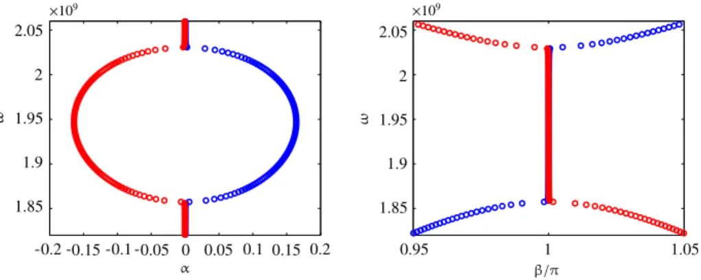
Fig. 2. The distribution of the eigenvalues which are close to and inside ofU.

Fig. 3. Dispersion diagrams ofαandβnear the stopping band.

matrix dimensions of Ciand Cbare n

=

63 960 and m

=

723, respectively. An example of computed reciprocal eigenpairs

near U at frequency

ω =

1

.

2757

/(

2

π) ×

1010is shown inFig. 2. The dispersion diagrams of the attenuation constant

α

and the propagation constant

β

associated with the eigenvalue

λ(ω)

are shown inFig. 3, for frequency

ω

around the stopping band, where the eigenpair most close to

−

1 on the complex plane is plotted.

4.1. Accuracy of structure-preserving eigensolvers

In this subsection, we compare the accuracy of the eigenpairs, computed by structure-preserving Algorithms 1, 2 and 7, respectively, for the GEP(8). Recall that the Krylov subspaceUjgenerated by the

⊤

-Hamiltonian matrixBis automatically

⊤

-isotropic inTheorem 3.2, and the subspacesZjandYj+1generated inTheorem 3.4are automatically

⊤

-bi-isotropic. As

(12)

Table 3

Convergent eigenvalues computed by T_NoSymp and GT_NoBiIso atω =1.2757/(2π) ×1010.

T_NoSymp GT_NoBiIso  λ,1 λ  −0.85175542558−0.52335156640ı −0.85175542559−0.52335156640ı −0.85228028786+0.52367406214ı −0.85228028785+0.52367406213ı −0.85175542557−0.52335156639ı −0.85175542556−0.52335156641ı −0.85228028787+0.52367406214ı −0.85228028786+0.52367406216ı −0.98999503056+0.00448884999ı −0.98999503056+0.00448884999ı −1.01008531402−0.00457994365ı −1.01008531402−0.00457994365ı −0.98999503056+0.00448884999ı −0.98999503056+0.00448884999ı −1.01008531402−0.00457994365ı −1.01008531402−0.00457994365ı

Fig. 4. The relative residual of the computed eigenpairs produced by different re-bi-isotropic processes in Algorithm 5 with shift valueτ = −0.99.

5 is important in maintaining the

⊤

-isotropic property. Moreover,Theorems 3.3and3.5both show that the multiplicities of eigenvalues of

(

K

,

N

)

are all even. In other words, no duplicate eigenpairs need to be computed theoretically when the

⊤

-isotropic property is kept during the computation. On the other hand, without the isotropic re-orthogonalization process, extra computation cost can arise in computing the duplicate eigenpairs. We would like to address this issue by numerical studies shown in the following. We also like to point out that the accuracy of the computed eigenpairs can be affected by different approaches in isotropic re-orthogonalization.

First, let us denote the algorithm that applying TSHIRA without the re-symplectic process as T_NoSymp and the algorithm that applying GTSHIRA without these re-bi-isotropic processes as GT_NoBiIso. In Table 3, the convergent eigenvalues obtained by T_NoSymp and GT_NoBiIso at frequency

ω =

1

.

2757

/(

2

π) ×

1010 are listed. Obviously, one can see that, in case only two eigenpairs

{

(λ

₁

, λ

−₁1

), (λ

₂

, λ

−₂1

)}

are needed here, the algorithms T_NoSymp and GT_NoBiIso return four convergent eigenpairs in which two of them are indeed the duplicated pairs.

Next, let us compare the accuracy of the computed eigenpairs obtained from three different isotropic re-orthogonalization approaches in GTSHIRA. One or two steps of re-bi-isotropic process can be performed by the for-loops in Steps 6–8 and 15–17.

To distinguish among various re-bi-isotropic processes, we use notations ‘‘FullIso’’, ‘‘zIsoY’’ and ‘‘yIsoZ’’ defined as follows:

•

FullIso: Algorithm 5 with two for-loops in Steps 6–8 and 15–17.

•

zIsoY: Algorithm 5 with one for-loop in Steps 6–8 and omitting for-loop in Steps 15–17.

•

yIsoZ: Algorithm 5 with one for-loop in Steps 15–17 and omitting for-loop in Steps 6–8.

To measure the accuracy of computed eigenpairs of(8), we consider the relative residual of an eigenpair

(λ, ψ)

where

ψ = [ψ

⊤

i

, ψ

⊤

ℓ

]

⊤which is defined as following:





Ci Ciℓ C_ir⊤ 0



ψ − λ



0 Cir C_i⊤_ℓ Cb



ψ



F





Ci Ciℓ C_ir⊤ 0





F

∥

ψ∥

_F

+ |

λ|





0 Cir C_i⊤_ℓ Cb





F

∥

ψ∥

_F

,

here

∥ ∗ ∥

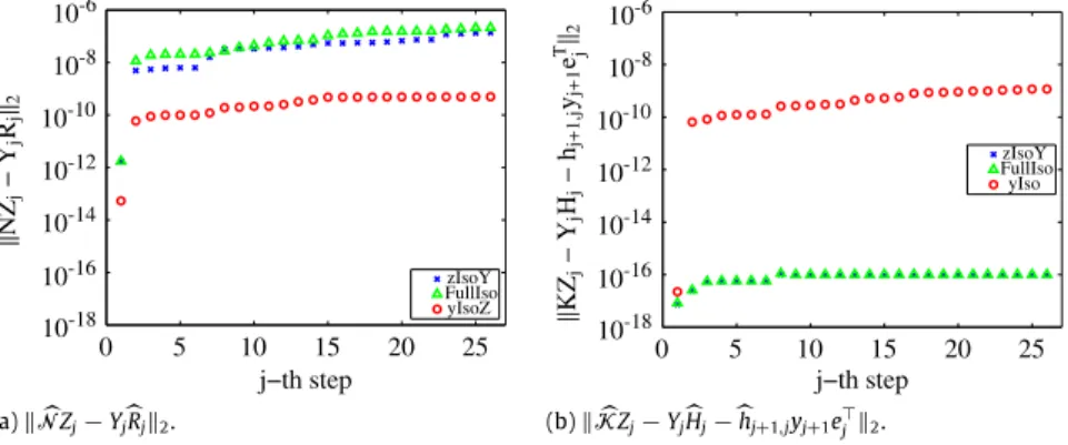
_Fis the Frobenius matrix norm. The relative residuals of the convergent eigenpairs computed by ‘‘FullIso’’, ‘‘zIsoY’’ and ‘‘yIsoZ’’ are shown inFig. 4. From the numerical results inFig. 4, we see that the accuracy of the convergent eigenpairs

(13)

(a)∥NZj−YjRj∥2. (b)∥KZj−YjHj−hj+1,jyj+1e⊤j∥2.

Fig. 5. The errors of the equalities in(18)and(19)for ‘‘FullIso’’, ‘‘zIsoY’’ and ‘‘yIsoZ’’. Table 4

CPU times (s) for GE_TSHIRA, GE_GTSHIRA, GE_SDA and GE_SA.

TSHIRA GTSHIRA SDA SA

Compute Ci=LU 191.31 191.31 191.31 191.31

Compute E1,E2,E2⊤E1 243.75 243.75

Compute A0,A1 533.94 533.94

Solve dense TPQEP 34.145

Solve Lx=b1 4.9850 4.9850 1.9940 1.9940 Solve Ux=b2 3.9775 3.9775 1.5910 1.5910 Solve U⊤ y=c2 33.597 27.998 Solve L⊤ y=c1 36.300 30.250 Compute E1d1,E⊤2c2 4.9150 4.9150 Compute E⊤ 1c1,E2d2 5.7930 4.8275

computed by ‘‘yIsoZ’’ is higher than those by ‘‘FullIso’’ and ‘‘zIsoY’’. This result can be explained from the accumulation of the errors in the equalities(18)and(19). Let

ξ

j,K

≡ ∥

K



Zj

−

Yj



Hj

−

hj+1,jyj+1e⊤j

∥

2and

ξ

j,N

≡ ∥

N



Zj

−

Yj



Rj

∥

2, denote these errors in

the jth iteration. The error

ξ

j,Ndepends on the accuracy of the solution of the linear systems in(23). If zjis reorthogonalized

toJY

¯

j, then the error produced by this reorthogonalization will reduce the accuracy of

ξ

j,N. Therefore,

ξ

j,N produced by

‘‘FullIso’’ and ‘‘zIsoY’’ are greater than that by ‘‘yIsoZ’’ as shown inFig. 5(a). On the other hand, the error

ξ

j,Konly depends on

the accuracy of matrix product vector and vector inner product. Obviously, the amount of

ξ

j,Kis much less than the amount

of

ξ

j,N. Consequently, even though the accuracy of

ξ

j,K can reduced by the errors from reorthogonalization yj+1toJZ

¯

jas

shownFig. 5(b), the reorthogonalization process ‘‘yIsoZ’’ is much accurate than the ‘‘FullIso’’ and ‘‘zIsoY’’ reorthogonalization processes.

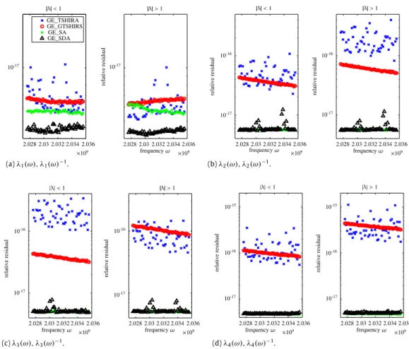
Finally, we compare the accuracy of the eigenpairs

(λ(ω),

u

(ω))

obtained from GE_SDA, GE_SA, GE_TSHIRA and GE_GTSHIRA with ‘‘yIsoZ’’ re-bi-isotropic process. The relative residuals resulted from these algorithms in computing four reciprocal eigenpairs

(λ

i

(ω),

ui

(ω))

, for i

=

1

, . . . ,

4, that are closest to

−

1 on the complex plane are plotted inFig. 6for

each frequency

ω

near the stopping band. Obviously, one can see that the accuracy of the eigenpairs obtained from GE_SDA and GE_SA are higher than those obtained by GE_TSHIRA and GE_GTSHIRA.

4.2. Comparison with computational costs

In this subsection, we discuss the computational costs of structure-preserving Algorithms 1, 2 and 7 in computing m

=

5 desired eigenpairs. Our numerical results show that the desired eigenpairs are convergent within 5m

⊤

-isotropic Arnoldi steps without restart for GE_TSHIRA and GE_GTSHIRA. On the other hand, it requires total 18 iterations to obtain a convergent Xkin Steps 3–6 for the SDA algorithm. As we mentioned in Section3.3, the number of forward and backward

substitutions needed for GE_TSHIRA and GE_GTSHIRA is only about half the amount of these substitutions that needed to transform the GEP into TPQEP in GE_SDA and GE_SA. Since only additional 25 forward substitutions and backward substitutions are needed in GE_TSHIRA and GE_GTSHIRA for solving linear systems Lx

=

b and Uy

=

c, we expect GE_TSHIRA

and GE_GTSHIRA to be more robust than GE_SA and GE_SDA. The following numerical results support this observation. To give an overall comparison for GE_SDA, GE_SP, GE_TSHIRA and GE_GTSHIRA, inTable 4, computational intensive items in these algorithms are listed in the first column and the sums of the CPU times for each associated item are listed in the other four columns. From the results inTable 4, the dominant computational costs in GE_TSHIRA and GE_GTSHIRA are the costs for computing E1

,

E2

,

E2⊤E1and LU factorization of Ci. For GE_SDA and GE_SA, the cost in computing the matrices A0

and A1of the TPQEP is the main cost comparing to the other costs. Obviously, the numbers shown inTable 4indicate that

(14)

(a)λ1(ω), λ1(ω)−1. (b)λ2(ω), λ2(ω)−1.

(c)λ3(ω), λ3(ω)−1. (d)λ4(ω), λ4(ω)−1.

Fig. 6. Relative residuals for GE_SDA, GE_SA, GE_TSHIRA and GE_GTSHIRA with shift valueτ = −0.89.

Fig. 7. CPU times for GE_SDA and GE_GTSHIRA.

and GE_GTSHIRA with frequency from 1

.

274

/(

2

π) ×

1010to 1

.

279

/(

2

π) ×

1010inFig. 7. FromFig. 7, one can see that the total CPU times needed in GE_SDA and GE_SA are 40% more than the CPU time needed in GE_TSHIRA and GE_GTSHIRA for computing 5 desired eigenpairs.

5. Conclusion

In this paper, we have discussed the structure-preserving methods for solving the generalized eigenvalue problem arising in the surface acoustic wave propagation on a simple resonator with an interdigital transducer (IDT) where electrodes are arranged periodically on piezoelectric substrates (PZT) such as 15°rotated Quartz. With given periodic boundary conditions,

(15)

the eigenvalues of the GEP appear in the reciprocal pairs

(λ, λ

−1

)

. In order to preserve the reciprocal relationship of the eigenvalues, the GEP is transformed to two types of T-palindromic quadratic eigenvalue problems, one with large coefficient matrices and the other with small coefficient matrices. The structure-preserving algorithms GE_SDA and GE_SA in Algorithms 1 and 2 are employed to solve the TPQEP (3)with small-size coefficient matrices and GE_TSHIRA and GE_GTSHIRA in Algorithm 7 are employed to solve the TPQEP(4)with large-size coefficient matrices.

In finding the five eigenpairs that are near U and close to

−

1, we observed duplicate eigenpairs appear when applying GE_TSHIRA and GE_GTSHIRA without re-symplectic and re-bi-isotropic processes, respectively. On the other hand, no duplicate eigenpairs are observed when re-symplectic and re-bi-isotropic processes are integrated in GE_TSHIRA and GE_GTSHIRA. Three different bi-isotropic processes in GE_GTSHIRA has been tested. We have found that using the re-bi-isotropic processes in Steps 15–17 of Algorithm 5 achieves the best accuracy. Moreover, our numerical results show that the relative residuals of the eigenpairs produced by GE_SDA/GE_SA and GE_TSHIRA/GE_GTSHIRA can be less than 10−17 and 10−15_{, respectively. Although the accuracy of GE_SDA and GE_SA is marginally higher than that of GE_TSHIRA and}

GE_GTSHIRA, we further found that the total CPU times required for computing the five desired eigenpairs by GE_SDA and GE_SA are about 40% more than that are required by GE_TSHIRA and GE_GTSHIRA. Therefore, by transforming the GEP into the TPQEP(4), the structure-preserving Arnoldi type algorithm GE_TSHIRA or GE_GTSHIRA with one ‘‘re-symplectic’’ or ‘‘re-bi-isotropic’’ processes provide an accurate and efficient way in finding the reciprocal eigenpairs of the GEP(1).

For further reading

[21,22].

Acknowledgments

The authors would like to thank reviewers’ careful reading and valuable suggestions to this manuscript. This work is partially supported by S.T. Yau Center of Chiao-Tung university, the National Science Council and the National Center for Theoretical Sciences in Taiwan. Chin-Tien Wu would like to thank the support from National Science Council under the grant number 99-2115-M-009-001. The second author was supported by the NSFC (No. 11101080) and the SRFDP (No. 20110092120023).

References

[1] T.-M. Huang, W.-W. Lin, C.-T. Wu, Structure-preserving Arnoldi-type algorithms for solving palindromic quadratic eigenvalue problems in leaky surface wave propagation. Technical report, National Center for Theoretical Sciences, National Tsing Hua University, Taiwan, Preprints in Mathematics 2011-2-001, 2011.

[2] A. Hilliges, C. Mehl, V. Mehrmann, On the solution of palindramic eigenvalue problems, in: Proceedings 4th European Congress on Computational Methods in Applied Sciences and Engineering, ECCOMAS, Jyväskylä, Finland, 2004.

[3] D.S. Mackey, N. Mackey, C. Mehl, V. Mehrmann, Structured polynomial eigenvalue problems: good vibrations from good linearizations, SIAM J. Matrix Anal. Appl. 28 (2006) 1029–1051.

[4] D.S. Mackey, N. Mackey, C. Mehl, V. Mehrmann, Vector spaces of linearizations for matrix polynomials, SIAM J. Matrix Anal. Appl. 28 (2006) 971–1004. [5] C. Schröder, A QR-like algorithm for the palindromic eigenvalue problem. Technical report, Preprint 388, TU Berlin, Matheon, Germany, 2007. [6] C. Schröder, URV decomposition based structured methods for palindromic and even eigenvalue problems. Technical report, Preprint 375, TU Berlin,

MATHEON, Germany, 2007.

[7] E.K-W. Chu, T.-M. Hwang, W.-W. Lin, C.-T. Wu, Vibration of fast trains, palindromic eigenvalue problems and structure-preserving doubling algorithms, J. Comput. Appl. Math. 219 (2008) 237–252.

[8] W.-W. Lin, A new method for computing the closed-loop eigenvalues of a discrete-time algebraic Riccatic equation, Linear Algebra Appl. 96 (1987) 157–180.

[9] R.V. Patel, On computing the eigenvalues of a symplectic pencil, Linear Algebra Appl. 188 (1993) 591–611.

[10] T.-M. Huang, W.-W. Lin, J. Qian, Structure-preserving algorithms for palindromic quadratic eigenvalue problems arising from vibration on fast trains, SIAM J. Matrix Anal. Appl. 30 (2009) 1566–1592.

[11] E.K-W. Chu, T.-M. Huang, W.-W. Lin, C.-T. Wu, Palindromic eigenvalue problems: a brief survey, Taiwan J. Math. 14 (3A) (2010) 743–779.

[12] S. Zaglmayr, Eigenvalue problems in saw-filter simulations. Diplomarbeit, Institute of Computational Mathematics, Johannes Kepler University Linz, Linz, Austria, 2002.

[13] C.K. Campbell, Surface Acoustic Wave Devices for Mobile and Wireless Communications, Academic Press, INC., 1998.

[14] M. Mohamed EL Gowini, W.A. Moussa, A finite element model of a mems-based surface acoustic wave hydrongen sensor, Sensors 10 (2010) 1232–1250.

[15] M.B. Angel, M.I. Rocha-Gaso, M.I. Carmen, A.V. Antonio, Surface generated acoustic wave biosensors for detection of pathogens: a review, Sensors 9 (2009) 5740–5769.

[16] H. Allik, T. Hughes, Finite element method for piezoelectric vibration, Int. J. Numer. Methods Eng. 2 (1970) 151–157.

[17] M. Buchner, W. Ruile, A. Dietz, R. Dill, FEM analysis of the reflection coefficient of SAWS in an infinite periodic array, in: Proc. IEEE Ultrason. Symp., 1991, pp. 371–375.

[18] M. Koshiba, S. Mitobe, M. Suzuki, Finite-element solution of periodic waveguides for acoustic waves, IEEE Trans. Ultrason. Ferroelectr. Freq. Control 34 (4) (1987) 472–477.

[19] R. Lerch, Simulation of piezoelectric devices by two- and three-dimensional finite elements, IEEE Trans. Ultrason. Ferroelectr. Freq. Control 37 (2) (1990) 1990.

[20] V. Mehrmann, D. Watkins, Structure-preserving methods for computing eigenpairs of large sparse skew-Hamiltonian/Hamiltonian pencils, SIAM J. Sci. Comput. 22 (2001) 1905–1925.

[21] G.W. Stewart, A Krylov–Schur algorithm for large eigenproblems, SIAM J. Matrix Anal. Appl. 23 (2001) 601–614.