行政院國家科學委員會專題研究計畫 成果報告
違約風險的經濟因素與 Levy 過程下之動態違約評價模型及
預警系統(第 2 年)
研究成果報告(完整版)
計 畫 類 別 : 個別型 計 畫 編 號 : NSC 98-2410-H-004-064-MY2 執 行 期 間 : 99 年 08 月 01 日至 100 年 07 月 31 日 執 行 單 位 : 國立政治大學金融系 計 畫 主 持 人 : 廖四郎 計畫參與人員: 博士班研究生-兼任助理人員:李嘉晃 報 告 附 件 : 出席國際會議研究心得報告及發表論文 處 理 方 式 : 本計畫可公開查詢中 華 民 國 100 年 10 月 11 日
違約風險的經濟因素與 Levy 過程下之動態違約評價模型及預警系統
計畫類別:
■
個別型計畫 □整合型計畫
計畫編號:
NSC 98-2410-H-004-064-MY2
執行期間: 99 年 8 月 1 日至 100 年 7 月 31 日
執行機構及系所:國立政治大學金融系
成果報告類型(依經費核定清單規定繳交):□精簡報告
■
完整報告
本計畫除繳交成果報告外,另須繳交以下出國心得報告:
□赴國外出差或研習心得報告
■
赴大陸地區出差或研習心得報告
□出席國際學術會議心得報告
□國際合作研究計畫國外研究報告
處理方式:
除列管計畫及下列情形者外,得立即公開查詢
涉及專利或其他智慧財產權,□一年□二年後可公開查詢
中 華 民 國 100 年 10 月 11 日
行政院國家科學委員會專題研究計畫成果報告
違約風險的經濟因素與 Levy 過程下之動態違約評價模型及預警系統 計畫編號:NSC 98-2410-H-004-064-MY2 執行期間: 99 年 8 月 1 日至 100 年 7 月 31 日 主持人:廖四郎 國立政治大學金融學系 AbstractSince the subprime crises occurred and the systematic and idiosyncratic risks are jointly affecting the default events, this study sets a system of pricing credit derivatives involving both the macro and firm-specific factors. In macroeconomic part, through the Kalman Filter and Gibbs sampling, one can capture the fundamental of macroeconomic sectors. In the microeconomic part, when the potential variable is lower than some barrier, it triggers the default. The Variance Gamma distribution describes the financial condition presenting kurtosis and skewness. Under this setting, we price credit default swaps.
Key words: Credit Default Swaps; Levy process; Derivative Pricing; Bayesian Statistics
中文摘要
個別公司違約事件受到系統性及非系統性風險的影響,本文在同時考慮總體及個 別公司環境下,建構包含兩者之信用風險的評價模型。在總體經濟環境方面,使 用 Gibbs 及 Kalman Filter 之狀態空間模型縮減總體及財務變數,描述總體經濟環 境的變化以決定違約強度,所以狀態空間模型賦予縮減式模型更多的經濟意涵。 在個體經濟環境方面,當個別潛在變數低於某個界限時將引發違約事件發生。由 於布朗運動無法完全描述市場情況,進一步採用 Variance Gamma 過程,更能符 合真實違約情況。最後,我們在這個架構下,評價信用違約交換之信用價差。 關鍵字: 狀態空間模型;Variance Gamma 過程;信用違約交換
1. Introduction
Since the subprime financial crises caused the financial activity to collapse and triggered a series of economic recession, these crises made investors lose their confidence in securitization and credit-related products. In order to renew investors’ confidence, this paper will attempt to construct a system including the whole credit risk and as far as possible to capture the default risks with reality reflecting the economic and firm-specific phenomena.
Models of credit risk fall into two categories: the structural-form approach and the reduced-form approach. The original idea of the structural-form approach is inspired by Merton (1974). With the framework of the structural-form model, the default time is defined as the first crossing time of the asset value through a default triggering barrier (Black and Cox, 1976; Leland, 1994; Longstaff and Schwartz, 1995). In the reduced-form approach, the credit events are specified in terms of some exogenous process. This model is only concerned with the random default time, which is also determined by the default intensity ( Jarrow and Turnbull, 1995; Lando, 1998 ). The shortcoming of the reduced-form approach is the lack of the economic meaning because the default intensity is exogenous.
In the finance literature, the market model is popularly used for the description of stock behavior. This model divides the overall risk into systematic and firm-specific risks. Drawing from the idea of this method, we assume the overall default risk of each entity is the sum of the two component risks.
For the systematic risk of macroeconomic condition, Wu and Zhang (2008) suggested that the default intensity is affected by the macroeconomic environment. Thus, we use the state-space model to extract from the economic and financial variables to describe the dynamics of the state vector concerning the economic condition. Also, Jarrow (2001) proposed an economic environment to determine the default intensity, i.e., the systematic risk is assessed by the economic data. Since the economic recession is implied in the economic variables, the state-space model tends to correspond to the subprime financial crises. Hence, our model is more reasonable than the other reduced-form models.
When estimating the parameters in the state-space model, we use the Bayesian method to obtain the posterior distribution to improve the robustness of the parameter estimates. This distribution is achieved by sampling and the prior distribution offers the parameters before. The Markov chain Monte Carlo (MCMC) is supported by Metropolis et al. (1953) involving the simulation of an appropriately constructed Markov chain that can converge to the posterior density. The Gibbs sampling is one of the simple method of MCMC since this method considers the full conditional distribution that makes it easy to generate the parameters. (Geman and Geman, 1984;
Gelfand and Smith, 1990; Gelfand et al., 1990).
In the firm-specific risk of microeconomic condition, we apply the idea from the structural-form approach. In the structural-form models, previous research assumes that the return of asset value follows a lognormal distribution. However, empirically, the financial data have shown the distribution with fat tail and skewness. The Lévy process, developed by Lévy, can capture the jump component which tends to fit the market situation well. Recently, the Lévy process is widely discussed in the valuation of derivatives (Madan et al., 1998; Hirsa and Madan, 2004; Cariboni and Schouten, 2007). Thus, the Variance Gamma (VG) process, which is one of the Lévy model suggested by Madan et al. (1998), has three parameters that can control the skewness and kurtosis of the distribution. Cariboni and Schoutens (2007) supported that the asset value follows a VG process that determines default risks. Since the firm-specific risk of a firm excludes the systematic risk, we don’t use the asset value as the variable just like the traditional structural-form approach. Thus, we define this variable as the potential variable which is used to measure the firm-specific risk. The potential variable is unobserved to imply the firm-specific risk that the systematic risk can’t capture. In this paper, we set a system that combines the systematic and idiosyncratic default risks to price a single-name credit default swap (CDS). In empirical part, we calibrate the CDS spreads to fit the market prices. After the calibration, the joint default probabilities can be easily obtained to price more complicated products. The rest of the paper is organized as follows. Section 2 discusses the state-space model with Kalman Filter and the estimation technique. Section 3 discusses the Lévy process. Section 4 studies the systematic and the firm-specific risks and denotes the valuation of the credit derivative products. Section 5 describes the empirical results and the conclusion.
2. The State-Space model 2.1 The Kalman Filter
Since the prices of credit derivatives are influenced by the economic environment, we need to draw the systematic information to reflect the reality condition. This idea is mainly originated from exploratory factor analysis (EFA), which extracts several variables that sufficiently represent the data. Similarly, because the market has too much information, the state-space model typically deals with this problem. The powerful tool used is the Kalman Filter, which is a useful tool to express a dynamic system for sequentially updating a linear projection of the system.
Following Wu and Zhang (2008), we assume that the vector of state variables E t follows an Ornstein-Unlenbeck process that is also a dynamic equation. Also, in order to price derivatives, we assume there exists a filtered probability
space{Ω,F,P,(Ft)0≤t≤T}.In this probability space,E is a Markov process. Thus, the t dynamics of the state vector are as follows:
dEt =−ϕEtdx+dWt, (1) whereW is an n-dimensional standard Brownian motion. t
For identification purposes, we let the long-run mean of the state vector be zero andϕ be the positive diagonal matrix that determines the mean-reversion speed of the state vector. Consider Equation (1) as discrete, it is a first order vector autoregression model denoted as VAR(1), which is written as:
Et =FEt−1+πt, (2) whereF =exp(−ϕΔt),πtis a Gaussian distribution with zero mean and covariance matrix Q andΔtdenote the discrete time interval.
Equation (2) is also called the transition equation which describes the dynamics of the state variables.
Next, we collect some useful macroeconomic series data, including economic and financial variables, such as the gross domestic product (GDP), consumer price index (CPI) and the house price index (HPI), etc. Then, these variables are observed data that are denoted asY whose dimension is m which is larger than the number of state t variables n. Thus, we can construct a measurement equation that relates observed data and unobserved state variables. This equation is written as follows:
Yt =HEt +δt, (3) whereδtis a Gaussian distribution with zero mean and covariance matrixR.For the simple estimation, let the matrixR is a diagonal matrix withRii =σi2.Also, we assume the errors of measurement and transition equation are independent.
In the Kalman Filter approach, the prior state estimate of the state vector at time t
given previous information isEˆt|t−1,andEˆ is the posterior estimate at time t, the prior t|t
and posterior estimate error can be defined aset|t−1andet|trespectively:
1 | 1 |t− = t − ˆtt− t E E e , et|t =Et −Eˆt|t.
Also, the prior and posterior estimate error covariance are given by
Pt|t−1 =E[et|t−1etT|t−1],Pt|t =E[et|tetT|t].
The goal of the Kalman Filter is to minimize the difference between the predicted
measurementsHEˆt|t−1and observed dataY Thus, the posterior state estimate is the t.
observed dataY and a measurement predictiont HEˆt|t−1. It can be expressed as follows: ). ˆ ( ˆ ˆ 1 | 1 | |t = tt− + t t − tt− t E K Y HE E (4)
Also, the weight called Kalman gainK is to minimize the error covariance of the t posterior estimate, thus
Kt =Pt|t−1HT(HPt|t−1HT +R)−1. (5) The Kalman Filter algorithm calculates the time and measurement updates. After the two steps, the algorithm is repeated with the previous posterior estimates used to predict the new prior estimates. This recursive way is one of the appealing features of the Kalman Filter. However, we need to estimate the state-space model parameters using the Bayesian statistics because the method generates the parameter estimates not affected by the initial values.
2.2 The Gibbs Sampling Approach
Bayesian analysis has been applied in statistical analysis. Ross (2006) compared the estimates using maximum likelihood estimates (MLE) with Bayesian estimates and thus founded in some cases MLE is irrational.
There are several reasons for using the Bayesian method rather the classical one. First, although the MLE can asymptotically converge to the true parameters, however, there are too many parameters to estimate in our model and the solutions of the MLE are significantly dependent on the initial values. Second, some parameters are limited to be larger or less than zero. Others are between 0 and 1. Due to the restrictions, we have to consider some specific distribution such as inverse variance gamma distribution, uniform distribution, and etc… Due to these reasons, the Bayesian method is more efficient and robust than the classical statistical approach. Next, we will introduce the Bayesian estimates and explain how to use it.
In the Bayesian approach, both the model’s parameters and the state variables are treated as random variables. In addition, the feature of the Gibbs sampling makes Bayesian approach in the state-space model easy to implement. The Gibbs sampling is introduced by Geman and Geman (1984). The Gibbs sampling algorithm is one of the simplest Markov chain Monte Carlo simulation methods for joint and marginal distributions by sampling from conditional distributions. Gelfand and Smith (1990) demonstrated the Gibbs algorithm for a range of problems in Bayesian analysis. Tanner and Wong (1987) discussed in the context of missing data problem. Hence, the basic idea of Gibbs sampling is that the unobserved state variables along with the parameters can be served as the missing data, and they can be generated via the Monte
Carlo simulation of Gibbs sampling.
Letθ be the parameter fori i=1,2,Kn , j is the number of generated random sample, f(θi |⋅,Y)is the conditional distribution, whereYis the observed variables.
Then, we will introduce the procedure of the Gibbs sampling. The Gibbs sampling algorithm is such that
1. Given an initial valuesθ(0) ={θ1(0),...,θn(0)}
2. Repeat for j=1,2,...,n0 +M Generate 1( ) j θ from f(θ1 |Y,θ2(j−1),θ3(j−1),...,θn(j−1)) Generate ) ( 2 j θ from f(θ2 |Y,θ1(j−1),θ3(j−1),...,θn(j−1)) M Generate ) (j n θ from f(θn |Y,θ1(j),...,θn(−j1))
3. Continue until all values are replaced by new ones.
For the Gibbs simulation, the following two steps are iterated until the convergence is succeeded.
1. Conditional on the model’s parameters and the economic and financial time
series data, generate the state variables
2. Conditional on the state variables and the economic and financial time series
data, generate the model’s parameters.
Then, one can construct the Gibbs sampling approach and obtain the state variables and parameters. The following two sections discuss how to generate them.
2.2.1 Generating the State Variables
There are two alterative ways to generate the state variables given the data and parameters. One is the singlemove Gibbs sampling, suggested by Carlin et al. (1992), generating the state variables one element at a time. Carter and Kohn (1994) generated the whole state variables called multimove Gibbs sampling that are more efficient and faster convergence than the other one. Thus, we employ the Carter and Kohn’s multimove Gibbs sampling approach.
Let T
T
T Y Y Y
Y~ =[ 1 2... ] be the observed data at time T,
T T
T E E E
the state vector at time T. The parameters are set to beΦ =[ϕ,H,R].This section is purposed to generate the state variables from the joint distribution given by
(~ |~ , ) (~ | ) ( | ,~). 1 1 1
∏
− = + = Φ T t t t t T T T T Y p E Y p E E Y E p (6)The state-space model is linear and are Gaussian distributed, the distribution of
T T Y
E |~ andEt Et Yt
~ ,
| +1 fort= T −1,K,1are all Gaussian:
ET |Y~T ~N(ET|T,PT|T), | ,~ ~ ( , ), 1 1 |, , | 1 + + + t ttEt ttEt t t E Y N E P E where ), ~ | ( ), ~ | ( | |T T T TT T T T E E Y P Cov E Y E = = ), ( ) ( ) ~ , | ( | 1 1 | | | 1 , | 1 t t t T t t T t t t t t t t E t t FE E Q F FP F P E Y E E E E t − + + = = + − + + , ) ( ) ~ , | ( | 1 | | | 1 , | 1 t t T t t T t t t t t t t E t t FP Q F FP F P P Y E E Cov P t − + + − = = + and 1 , |tEt+ t E and 1 , |tEt+ t
P are obtained from the previous Kalman Filter calculation.
2.2.2 Generating the Parameters
Since the measurement and transition equations of state-space model are both linear regression model, we consider a simple one to generate the parameters.
y = xβ +ε,
where the data y andε areT×1vectors, andxis aT× matrix. K
In the Gibbs sampling algorithm, we need to specify the distributions ofβandσ2. First, the priorβ follows a normal distribution as
β ~ N(β0,Σ0).
Second, the priorσ2follows an inverse-gamma distribution as ). 2 1 , 2 1 ( ~ 0 0 2 δ σ IG v
In this case, if one takesβ andσ as the two blocks,2 the full conditional density ofβ ish(β| y,σ2),which can be derived as
, ) ˆ ( ) ˆ ( 2 1 exp ) , | ( 2 ' 11 ⎩ ⎨ ⎧ ⎭ ⎬ ⎫ − Σ − − ∝ β β − β β σ β y h
where ˆ ( 0 2 ), 1 0 1 x y T − − + Σ Σ = β σ β and Σ1 =(Σ−01+σ−2xTx)−1.
Thus, the full conditional density ofβis multivariate normal.
The full conditional density ofσ2is the densityh(σ2 | y,β)and can be shown to be an updated inverse-gamma distribution:
), 2 , 2 ( ~ ) , ( | 1 1 2 β ν δ σ y IG where ( ) ( ) , 0 1 0 1 β β δ δ ν ν x y x y T T − − + = + =
Both full conditional densities are thus tractable.
3. Lévy Process
In the finance literature, the normality assumptions are usually applied. However, many empirical studies have shown that the log-returns aren’t normal and that the skewness is 0 and the kurtosis is 3. The Lévy process is applied because it can capture the empirical distributions. In addition, the Variance Gamma (VG) process is one of the Lévy process. Hence, we consider a VG process corresponding to the dynamics of the potential variable. In what follows, we briefly introduce this process.
3.1 The Variance Gamma Process
Madan et al. (1998) proposed the Variance Gamma (VG) process, which is obtained by Brownian motion at a random time change given by a Gamma process. That is to say that the VG process is considered as a subordinated Brownian motion. This process has two additional parameters dominating the skewness and kurtosis of the log-return distribution. In our model, we use the potential variable following the VG process which is similar to the firm value. Next, we introduce some properties of the VG process.
The characteristic function of theVG(σ,v,θ)process is given by
) , 2 1 1 ( ) , , , , ( 2 2 tv VG x t v ix v x v − + − = θ σ θ σ φ (7) whereφ(⋅)is the characteristic function.
⎪⎩ ⎪ ⎨ ⎧ > − < = − − 0 , ) exp( 0 , | | ) exp( ) ( 1 1 x dx x Mx C x dx x Gx C dx vVG where = 1 >0, v C ) 0, 2 1 2 1 4 1 ( 2 2 + 2 − 1 > = − v v v G θ σ θ ) 0. 2 1 2 1 4 1 ( 2 2 + 2 + 1 > = − v v v M θ σ θ
Also, A VG process has no Brownian motion part and its Lévy triplet is given by )) ( , 0 , (γ vVG dx , where ( exp( ) 1) (exp( ) 1)). MG G M M G C − − − − − − = γ
With the three parameters of the VG process, the characteristic function ofXt(VG)is as
follows: ) . ) ( ( 2 C VG x ix G M GM GM + − + = φ (8) Thus, we will refer the VG process asVG(C,G,M).
Madan et al. (1998) stated that the VG process could be expressed as the difference of two independent Gamma process, i.e.:
Xt(VG) =Gt(1) −Gt(2),
where G(1) ={Gt(1),t≥0} is a Gamma( ba, ) process with parameters a=C and ,
M
b= whereasG(2) ={Gt(2),t ≥0}is also aGamma( ba, ) process with parameters
C
a= andb=G.Also, the VG process is also defined as time-changed Brownian motion with drift term. The subordinated Brownian motion is expressed as
Xt(VG) =θGt +σWt, (9) whereG be a Gamma process with parameterst = = 1 >0
v b
a ,W denotes a standard t
Brownian motion.
Thus,θ controls the drift term of the Brownian motion. Whenθ =0, thenG=M, so the distribution is symmetric.vis the variance of the subordinator, which primarily
controls the kurtosis. The statistics of the VG process with three parameters are in Table 1.
<Table 1 here>
Noticeably, Table 1 shows the skewness and kurtosis are controlled byvandθ . Furthermore, negative values ofθ leads to negative skewenss.
3.2 The Monte Carlo Simulation of VG Process
On a filtered probability space{Ω,F,Q,(Ft)0≤t≤T},the dynamics of the potential variable are given as an exponential Lévy process of the VG process.
Under the risk-neutral measure, it is described as follows:
St =S0(exp(r−q)t+Xt +τt), (10) whereX is a VG process,t r is the continuously compounded interest rate, q is a continuous dividend yield,τ is the adjusted drift term, which is set to be
). 2 1 1 log( 2 1 v v v θ σ τ = − − −
To get the efficient simulation of the VG process, we will sample the different independent Gamma processes. Equation (7) can be written as the product of the following two characteristic functions,
(t,x, , ) (1 i x)−tv, + + + + + = − α β β α φγ and (t,x, , ) (1 i x)−tv, − − − − − = + α β β α φγ with parameters , . 2 2 2 2 2 v v ± ± ± = ± + = θ β α σ θ α
4. The Overall Default Risk of the System
Since the default risks are divided into two components. One is the systematic risk, and the other is the firm-specific risk. Thus, we separately introduce the two risks in this section.
4.1 The Systematic Default Risk
probability. Under the state-space model, we draw the three state variables from the systematic information. Moreover, for examining the effect of the macroeconomic condition on the default intensity and observing the credit condition with the shift of the economic and financial environment, following Wu and Zhang (2008), we assume the default intensity is an affine function of the dynamics of the state vector, it follows
λ(Et)=αλ +βλTEt, (11) Also, under the risk-neutral measureQ , the dynamics of the state vector follow an Ornstein-Unlenbeck process such that
dEt =κ(ξ −Et)dt+dWtQ. (12) If the intensity is stochastic, the systematic survival probability at time T can be calculated as
PS(T)=Q(τ >T |Ft)=exp(−α(T)−β(T)TEt), (13) whereτ denotes the default time, and the solution ofα(T)andβ(T)are given as the following Riccati ordinary differential equations:
, 2 ) ( ) ( ) ( ) ( ' T T T T T Tκξ β β β α α = λ − − β'(T)=βλ −κTβ(T),
with the boundary conditionα(0)=0 and β(0)=0.The coefficientαλ and βλ in Equation (11) are achieved by solving these differential equations through the numerical calculation.
4.2 The Firm-specific Default Risk
Regarding to the previous research of structural-form approach, Merton (1974) first proposed a model to measure default probabilities. However, this model assumes the firm asset value follows a lognormal distribution. We adopt a Lévy process of structural-form approach to measure the firm-specific risk. The main idea of our study is suggested by Cariboni and Schoutens (2007). In our model, since we have already captured the systematic risk, the firm-specific risk is the remaining risk which the systematic risk is excluded, the dynamics of the potential variable which triggers the firm-specific default event. Hence, the potential variable implies that this variable is used to indicate that the firm-specific risk which the systematic risk can’t capture and that isn’t included in the systematic risk.
Given the filtered probability space{Ω,F,Q,(Ft)0≤t≤T},the potential variable can be described by a Lévy process, which follows an exponential VG process such that
St =S0exp(Xt), (14) whereX is the VG process at time t. t
In the structural-from approach, the default event occurs when the firm value is lower than some barrier. Then, we assume the potential variable hits the triggering barrierB . Thus, the default event is triggered if
St =S0exp(Xt)≤ B. or equivalently if log( ). 0 S B Xt ≤
As mentioned above, we define the occurrence of the default, the idiosyncratic survival probability at time T is measured as follows:
( ) ( ) (min ) (min log( )).
0 0 0 S B X Q B S Q T Q T P t T t t T t I = > = > = > ≤ ≤ ≤ ≤ τ (15)
4.3 The Overall Default Risk
First, we consider a regression that connects the systematic and idiosyncratic risks, which was introduced by sharp (1963) and is called market model. The purpose of this model is to separate the market from the firm-specific risk. Formally,
Ri =αi +βiRM +εi, (16) whereR denotes the return of each stock,i RM denotes the market return,βiis the sensitivity ofR toi RM,εistands for the residual of this model.
Second, we assume the systematic and firm-specific risks are independent, so the system of the overall credit risk is jointly determined by the two risks. The overall survival probability can be analyzed by these two components simultaneously at time T. Therefore,
PiJ(T)=1−[wi(1−PiS(T)+(1−wi)(1−PiI(T))], (17) wherewi =αβistands for the weight of the systematic risk,α stands for the common factor that affects whole entities,βirepresents the characteristic of each entity.
4.4 The Valuation of the Credit Derivatives
The Dow Jones CDX North American Investment Grade (DJ CDX NA IG) index consists of 125 corporations whose credit default swaps (CDSs) are actively traded. A typical CDS contract is designed to against the default risk. A protection buyer pays a fixed credit spread s to a protection seller at each payment datet1,t2,...,tn.Also, the protection buyer will receive payments1−R,whereR is the recovery rate when credit event occurs. In this framework, the present value of the regular payments for the protection seller as the first kind of premium leg:
( )( ) ( ), 1 1
∑
= − − = n i i i i i R s D t t t P t PLwhereD(ti)refers to the discount factor,P(ti)denotes the survival probability at time i
t . If the default event occurs at the middle time of each payment date, the present value of the accrual payments for the protection seller as the second kind of premium leg:
∑
= − − − − − + = n i i i i i i i A t t P t P t t t D s PL 1 1 1 1 )). ( ) ( )( )( 2 ( 2 1Then the payments for the protection buyer as the default leg:
)( ( ) ( )). 2 ( ) 1 ( 1 1 1
∑
= − − − + − = n i i i i i t P t P t t D R DLIf there is no arbitrage opportunity, the spread price is fair. That is to say the present value of the premium leg is equal to the present value of the default leg. Thus,
E(PLR +PLA)=E(DL).
The fair credit spread is calculated as follows:
. )) ( ) ( )( )( 2 ( 2 1 ) ( ) )( ( )) ( ) ( )( 2 ( ) 1 ( 1 1 1 1 1 1 1 1 1
∑
∑
∑
= − − − = − = − − − − + + − − + − = n i i i i i i i n i i i i i n i i i i i t P t P t t t t D t P t t t D t P t P t t D R s (18)5. Empirical Results and Conclusion
5.1 Macroeconomic Data Description and Estimation Results
Before pricing the CDX index, we draw some macroeconomic variables to reflect actual condition on the prices. The macroeconomic data are eleven series selected from March 1998 to March 2009, observed monthly or quarterly. All data come from the DataStream except the house price index (HPI). These variables are divided into three sectors including the real activity, inflation and credit sectors. The real activity and inflation sectors are needed to involve in our methodology suggested by Wu and Zhang (2008). The real economic activity consists of the gross domestic production (GDP), the industrial production (IP), the personal income (PI), and the unemployment. The consumer price index (CPI) and the producer price index (PPI) are incorporated to describe the inflation sector. Since the mortgage-related derivatives are the main components in the credit market, it is necessarily to concern this mortgage-related factor in pricing CDX index. After examining the credit market and previous literature, some variables are recognized to analyze the influence of the default intensity. Thus, the credit sector includes the HPI, the delinquency rate for subprime mortgage and whole market, and the foreclosure rate for subprime mortgage and whole market. All variables are measured by the year-over-year except the
delinquency and foreclosure rates. Table 2 summarizes the statistics of all economic and financial series.
<Table 2 here>
In the estimation of the state-space model, we use the Gibbs algorithm to obtain the parameters in measurement and transition equations. We simulate the Gibbs samples 10,000 times and select the first half of the samples to estimate parameters. The results are shown that the parameters tend to converge quickly and robust of simulated simples for each parameter. These parameters are displayed in Table 3.
<Table 3 here>
Variables from the real economic activity are positive except for the unemployment rate, which is negative. It closely coincides with the real economic situation. If the economy falls into recession, the GDP and IP diminish while the unemployment rises. All variables of the credit sector have positive coefficients except for the HPI. This result implies that the credit sector has negative influence on the HPI. This phenomenon corresponds to the true situation that higher house price makes the refinancing of mortgage loans easy and then the foreclosure and delinquency rates decrease.
5.2 The Calibration of the CDX Index and its Empirical Results
As mentioned in Equation (11) and Equation (12), the default intensity is linked with the macroeconomic environment. Before pricing the CDX index, the calibration is
necessary. To estimate these parametersΦs =[κ,ξ,αλ,βλ],we need to minimize the difference between market pricessMarket and model pricessModelto find the error minimization Φ =
∑∑
− i t Model t t Market t t s t s t s i i ( ) ( )] . [ min arg ˆ 2 , , , , ,ξαλβλ 1 1 κ (19) where iMarkett t j s, ,1 is the market CDS spread of each entityi from timet1to ,tj also,
Model t t i j s, , 1 is the
model CDS spread of each entityi fromt1to .t Thus, the estimated default intensity is j
λˆ(Et)=−0.0255+[−0.00497 0.0119 0.005]Et.
the CDX index prices are available. The results of the estimated parameters are also presented in Table 4.
<Table 4 here>
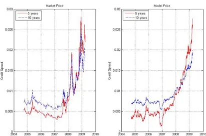
Then, we use these parameters to price CDX spreads for the most popular trading maturities of 5 years and 10 years. Figure 1 shows the difference between the market and the model prices. In reality, the market prices didn’t go up until the fist quarter of 2007, while the model market prices rapidly increase at the beginning of that year. The crisis made the market prices sharply increased in the beginning of 2008 and caused a peak in the middle of 2008. In contrast, the model prices increased steadily, coinciding with the weak economic condition. From the late 2008 to the early 2009, the market prices dropped quickly and then peaked again. However, the model prices still steadily increased.
<Figure 1 here>
5.3 The CDS spreads calibration and pricing
As mentioned before, the systematic component of default risk is measured by the state-space model from the macroeconomic series and we price the CDX index before. Then, the remaining parameters also need to be calibrated from the CDS spreads. Moreover, the parameters are calibrated by minimizing the difference between the market prices and the model prices given by
Φ =
∑∑
− j i Model t t i Market t t i I j j s s ] , [ min arg , , , , 2 , , ,σνθ 1 1 α (20) The APE is to measure the fitness of the model price. It can be calculated as1 | |, 1 , , 1 1
∑
= − = N j Model t t Market t t market N s s s APE j j (21)wheresmarketis the mean of the market CDS spreads.
According to the calibration of CDS prices in Equation (20), we will calibrate a series of CDS spreads on March 31, 2009. In Table 5, we report the market and model spreads. The calibration results show that the results fit the market prices well. In addition, Table 6 reports each estimated parameter of the whole corporations. Furthermore, each entity represents the skewness to the left.
<Table 6 here>
In order to investigate the microeconomic environment affecting the CDS prices, we show the movement of CDS spreads of Amgen and Walt Disney Corporations. Since we know that theβi’s of Amgen and Walt Disney Corporations are 0.698 and 1.036 respectively. Figure 3 displays the Walt Disney Corporation’s spreads change more significantly than Amgen since theβipresents the sensitivity of each entity to the macroeconomic situation, i.e., the largerβimakes the CDS prices move violently. That is to say the flat plane represents Amgen Corporation with smallerβiwhile the steep plane represents Walt Disney Corporation with largerβi.Moreover, when the variable of credit environment becomes larger, it means the delinquency and foreclosure rates increase which result in the increment of the CDS spreads. Therefore, our model is more intuitive than the traditional reduced-form approach and the state-space model gives the CDS prices more economic insight.
<Figure 2 here>
5.4 Conclusion
The subprime mortgage crisis occurred at the beginning of 2007 had lasted more than two years. This crisis is triggered by a dramatic rise in mortgage delinquency and foreclosure rates in the United States, with major negative shocks on banks and financial markets around the world leading to the collapse of the global financial system. The mortgage related financial derivatives such as MBS or CDO are involved in the crisis. The phenomenon forces us to find a more practical model to capture the credit risks that are implied in the default derivatives.
At the beginning of the crisis, investors wondered why the credit agencies didn’t reflect the real credit condition of each entity. At that time, all market indices became worse and the default rates were larger. By the end of 2008, the price of CDS or CDO rapidly increased and fluctuated significantly. Since the macroeconomic variables have crucial impact on the systematic default risk, it suggests us to adopt the state-space model to extract the variables that can represent the most systematic information of market to determine the systematic default risks. In estimation method, because of the robustness of the parameters using Gibbs sampling, we discard the MLE method that is significantly affected by the initial values. Thus, we use the state-space model with Kalman Filter and Gibbs sampling to obtain the real activity, inflation and credit state variables. Before the market prices increased at the end of 2008, the model prices reflected the weak economic condition that went up ahead and stably increased. Hence, the state-space model of related macroeconomic environment
is more realistic corresponding to the market condition.
In the idiosyncratic default risk, the default event is triggered by the firm-specific potential variable that is the first crossing of a default triggering barrier. Since the Brownian motion can’t capture the skewness and kurtosis of empirical financial distribution, we apply a VG process which is also a jump process. The VG process is more accurate than the Brownian motion adopted by traditional structural-form model such as the Merton model. With this improved process, it gives us a better model.
The idea of the market model proposed by Sharp (1963) is to jointly consider the systematic and the firm-specific risks. We use this concept to construct an overall default risk including these two component default risks which are independent. Then, we give some examples of pricing CDS using the overall default risk. Also, we show that the CDS spreads move simultaneously with the economic situation. In other words, more sensitivity to the economic condition makes the CDS prices increase. Although the reduced-form model can deal with more complicated structures, it is with less economic meaning than the structural-form model. As a result, we improve the shortcoming of traditional reduced-form model in systematic risk and adopt the structural-form model in firm-specific risk. Therefore, our model is more economically intuitive than the others even if we combine the reduced-form and structural-form models.
Figure 1: The comparison of Market and Model prices
The data period is from September 2004 to March 2009. The left hand is the 5-year and 10-year CDX prices of Market. The right hand is the 5-year and 10-year CDX prices of Model.
Figure 2: The impact of economic condition on the CDS spreads
The movement of CDS spreads of Amgen and Walt Disney Corporations affected by macro- economic is represented here.
Table1: Statistics of the VG process with three parameters(σ,v,θ) VG process VG(σ,v,θ) VG(σ,v,0) Mean θ 0 Variance σ2 θ2 v + σ2 Skewness 2 2 2 2 32 ) /( ) 2 3 ( σ θ σ θ θv + v +v 0 Kurtosis 3(1+2v−vσ4(σ2 +vθ2)−2) 3(1+ v)
This table describes the statistics of the Variance Gamma process. It also shows the skewness and kurtosis are controlled byvandθ. Furthermore, negative values ofθleads to negative skewenss.
Table 2: Statistics of all macroeconomics variables
Macroeconomic Variables Frequency Mean Standard Deviation Real Activity GDP Quarterly 5.1348 1.2859 IP Monthly 1.4842 3.3169 PI Monthly 4.3041 1.5375 Unemployment Monthly 4.7983 16.3913 Inflation CPI Monthly 2.7164 1.0417 PPI Monthly 3.7980 4.8925 Credit HPI Monthly 8.0689 10.0258 Delinquency-all Monthly 4.8311 0.7766 Delinquency-subprime Quarterly 12.9149 2.7799 Foreclosure-all Quarterly 0.4892 0.1933 Foreclosure-subprime Quarterly 2.0705 0.8289
The summary of all macroeconomic indices are represented in this table. The data period is from June 1998 to March 2009. All macroeconomic variables are reported as year-over-year percentage changes except for the foreclosure and delinquency rates.
Table 3: The estimation results of the state-space model Macroeconomic Variables H Rii GDP 0.7140 0.3624 IP 0.7884 0.2130 PI 0.3970 0.8166 Unemployment -0.8596 0.0754 CPI 0.8605 0.1592 PPI 0.8929 0.0998 HPI -0.8645 0.3563 Delinquency-all 1.0158 0.1122 Delinquency-subprime 1.0497 0.0543 Foreclosure-all 0.9578 0.2135 Foreclosure-subprime 0.9527 0.2185
This table presents the estimation results of the parameters in measurement and transitions equations. Every entry is the estimation.
Table 4: The estimation of these parameters on March 31, 2009
Date αλ βλ κ κξ
-0.0497 1.56 -0.9224
0.0119 1.6695 1.1002
2009-3-31 -0.0255
0.005 0.9380 1.3999
The parameters’ estimation of the default intensity is obtained using Equation (18) on March 31, 2009. The result is used by the calibration technique.
Table 5: Market spreads and the results of calibration
Company 1y 3y 5y 7y 10y Market 40 48 55 58 46 McDonalds Model 39 46 52 57 57 Market 53 64 73 77 72 Walt Disney Model 57 60 70 71 76 Market 73 79 85 80 77 Amgen Model 71 77 83 80 79
The comparison of market and model prices is shown in this table. There are three corporations.
Table 6: Results of estimated parameters Company β σ ν θ APE(%) McDonalds 0.63 0.0926 1.1260 -0.0763 7.28 Walt Disney 1.036 0.1000 0.7891 -0.1039 6.15 Amgen 0.698 0.0931 3.1626 -0.0612 2.05 1 . 0 = α
The estimated betas are used by Equation (16). Also, the other estimated parameters are obtained by Equation (20).
Reference
Ang, A and Piazzesi M., A no-arbitrage vector autoregression of term structure dynamics with macroeconomic and latent variables. J. Mone. Econ., 2003, 50, 745-787.
Black, F. and Cox, J.C., Valuing corporate securities: some effects on the bonds indenture provisions. J. Finance, 1976, 31, 351-367.
Bielecki, T. R. and Rutkowski, M., Credit Risk: Modeling Valuation and Hedging, 2002, (Springer-Verlag: Berlin, Heidelberg, New York).
Cariboni, J. and Schoutens W., Pricing credit default swaps under Lévy models. J. Computat. Finance, 2007, 10, 1-21.
Carlin, B. P., Polson N. G.., and Stoffer D. S., A Monte Carlo approach to nonnormal and nonlinear state-space modeling. J. Am. Statist. Asso., 1992, 87, 493-500.
Carter, C. K. and Kohn R., On Gibbs sampling for state space models. Biometri., 1994, 81, 541-553.
Cont, R. and Tankov P., Financial Modelling With Jump Processes, 2003 (Chapman & Hall/CRC).
Gelfand, A. E., Hills, S. E., Racine-Poon, A. and Smith A. F. M., Illustration of Bayesian inference in normal data models using Gibbs sampling. J. Am. Statist. Asso.,1990, 85, 972-985.
Gelfand, A. E. and Smith, A. F. M., Sampling-based approaches to calculating marginal densities. J. Am. Statist. Asso.,1990, 85,398-409.
Geman, S. and Geman D., Stochastic relaxation, Gibbs distribution and the Bayesian restoration of images. IEEE Trans. Pattern Ann., Machine Intell., 1984, 6,721-741. Hamilton, J. D., Time Series Analysis, 1994 (Princeton, New Jersey).
Hirsa, A., and Madan, D. B., Pricing American option under Variance Gamma. J. Computat. Finance, 2004, 7, 63-80.
Jarrow, R. A., Default parameter estimation using market prices. Finan. Analysts. J., 2001, 5, 74–92.
Jarrow, R. A., Turnbull, S. M., Pricing derivatives on financial securities subject to credit risk. J. Finance, 1995, 50, 59-85.
Lando, D., On Cox process and credit risky securities. Rev. Derivatives Res., 1998, 2, 99-120.
Lando, D., 2004, Credit Risk Modeling: Theory and Applications (Princeton and Oxford).
Leland, H. E., Corporate debt value, bond covenants, and optimal capital structure. J. Finance, 1994, 49, 987-1019.
Floating Rate Debt. J. Finance, 1995, 50, 789-819.
Madan, D. B., Carr P., and Chang E. C., The Variance Gamma process and option pricing. Euro. Finance Rev., 1998, 2, 79-105.
Merton, R., On the pricing of corporate debt: The risk structure of interest rates. J. Finance, 1974, 29, 449-470.
Metropolis, N., A. W. Rosenbluth, M. N. Rosenbluth, A. H. Teller, and Teller E., Equation of state calculations by fast computing machines. J. Chem. Phys., 1953, 21, 1087-1091.
Press S. J., 2003, Subjective and Objective Bayesian Statistics: Principles, Models, and Applications (John Wiley and Sons).
Ross, S. M., 2006, Introduction to Probability Models (Academic Press).
Schoutens, W., 2003, Lévy process in Finance: Pricing Financial Derivatives ( John Wiley and Sons).
Sharp, W. F., A simplified model for portfolio analysis. Manage. Science, 1963, 9, 277-293.
Shreve, S. E., 2008, Stochastic Calculus for Finance Ⅱ: Continuous-Time Models (Springer).
Tanner, M. A. and Wong, W. H., The calculation of posterior distribution by data augmentation. J. Am. Statist. Asso., 1987, 82, 528-540.
Wu, L. and Zhang F. X., A no-arbitrage analysis of macroeconomic determinants of the credit spread term structure. Manage. Science, 2008, 54, 1160-1175.
出差與研習心得
本人於 2011 年 7 月 22 日由台灣搭機赴中國大陸內蒙古呼和浩特,參加「2011 年中國金融工程年會暨金融工程與風險管理論壇」。於 7 月 22 日下午四點左右抵 位於內蒙古呼和浩特主辦單位內蒙古財經大學。晚上住宿於呼和浩特碧儷宮,並 與來自全中國的金融工程學教授與業者共敘晚宴。台灣方面的參加者除本人外, 另有數位台灣學者與金融研訓院院長許振明教授。7 月 23 日參加整天的研討會,本人發表論文「An Investigation on Specturm
Portfolio Strategy」。
此次參加該會,除增進兩岸學術交流的目的外,亦深覺大陸地區之學者正拼力
追趕西方的研究,並擁有其自有的哲學判斷標準,不盡與台、美、日之學術觀點
完全相同。本人除與學術界人士接觸交流外,亦與大陸地區之證監會與業界人士
國科會補助計畫衍生研發成果推廣資料表
日期:2011/05/25國科會補助計畫
計畫名稱: 違約風險的經濟因素與Levy 過程下之動態違約評價模型及預警系統 計畫主持人: 廖四郎 計畫編號: 98-2410-H-004-064-MY2 學門領域: 財務無研發成果推廣資料
98 年度專題研究計畫研究成果彙整表
計畫主持人:廖四郎 計畫編號:98-2410-H-004-064-MY2 計畫名稱:違約風險的經濟因素與 Levy 過程下之動態違約評價模型及預警系統 量化 成果項目 實際已達成 數(被接受 或已發表) 預期總達成 數(含實際已 達成數) 本計畫實 際貢獻百 分比 單位 備 註 ( 質 化 說 明:如 數 個 計 畫 共 同 成 果、成 果 列 為 該 期 刊 之 封 面 故 事 ... 等) 期刊論文 0 0 100% 研究報告/技術報告 0 0 100% 研討會論文 1 0 100% 篇 論文著作 專書 0 0 100% 申請中件數 0 0 100% 專利 已獲得件數 0 0 100% 件 件數 0 0 100% 件 技術移轉 權利金 0 0 100% 千元 碩士生 0 0 100% 博士生 1 0 100% 博士後研究員 0 0 100% 國內 參與計畫人力 (本國籍) 專任助理 0 0 100% 人次 期刊論文 1 0 100% 研究報告/技術報告 0 0 100% 研討會論文 0 0 100% 篇 論文著作 專書 0 0 100% 章/本 申請中件數 0 0 100% 專利 已獲得件數 0 0 100% 件 件數 0 0 100% 件 技術移轉 權利金 0 0 100% 千元 碩士生 0 0 100% 博士生 1 0 100% 博士後研究員 0 0 100% 國外 參與計畫人力 (外國籍) 專任助理 0 0 100% 人次其他成果
(
無法以量化表達之成 果如辦理學術活動、獲 得獎項、重要國際合 作、研究成果國際影響 力及其他協助產業技 術發展之具體效益事 項等,請以文字敘述填 列。) 無 成果項目 量化 名稱或內容性質簡述 測驗工具(含質性與量性) 0 課程/模組 0 電腦及網路系統或工具 0 教材 0 舉辦之活動/競賽 0 研討會/工作坊 0 電子報、網站 0 科 教 處 計 畫 加 填 項 目 計畫成果推廣之參與(閱聽)人數 0國科會補助專題研究計畫成果報告自評表
請就研究內容與原計畫相符程度、達成預期目標情況、研究成果之學術或應用價
值(簡要敘述成果所代表之意義、價值、影響或進一步發展之可能性)
、是否適
合在學術期刊發表或申請專利、主要發現或其他有關價值等,作一綜合評估。
1. 請就研究內容與原計畫相符程度、達成預期目標情況作一綜合評估
■達成目標
□未達成目標(請說明,以 100 字為限)
□實驗失敗
□因故實驗中斷
□其他原因
說明:
2. 研究成果在學術期刊發表或申請專利等情形:
論文:□已發表 ■未發表之文稿 □撰寫中 □無
專利:□已獲得 □申請中 ■無
技轉:□已技轉 □洽談中 ■無
其他:(以 100 字為限)
3. 請依學術成就、技術創新、社會影響等方面,評估研究成果之學術或應用價
值(簡要敘述成果所代表之意義、價值、影響或進一步發展之可能性)(以
500 字為限)
In this proposal,although the reduced-form model can deal with more complicated structures, it is with less economic meaning than the structural-form model. As a result, we improve the shortcoming of traditional reduced-form model in systematic risk and adopt the structural-form model in firm-specific risk. Therefore, our model is more economically intuitive than the others even if we combine the reduced-form and structural-form models.We set a system that combines the systematic and idiosyncratic default risks to price a single-name credit default swap (CDS). In empirical part, we calibrate the CDS spreads to fit the market prices. After the calibration, the joint default probabilities can be easily obtained to price more complicated products.