微機械麥克風之最佳化設計及其陣列於3D聲場重建之實現

國 立 交 通 大 學

機械工程研究所

碩 士 論 文

微機械麥克風之最佳化設計及其陣列於

3D 聲場重建之實現

Optimal Design and Experimental Verification of a

MEMS Microphone Array for 3D Hearing

研 究 生：林振邦

指導教授：白明憲

中華民國九十三年六月

微機械麥克風之最佳化設計及其陣列於

3D 聲場重建之實現

研究生 : 林振邦 指導教授 : 白明憲

國立交通大學機械工程學系

摘要

電容式麥克風有較高的靈敏度與較平坦與寬廣的頻率響應，因此被廣泛的應 用於各種場合。利用微機電技術可將體積微小化，卻不失其性能，並可降低雜散 電容的影響。文中探討微機械電容式麥克風的動態行為分析，並利用田口實驗法 (Taguchi method)與遺傳演算法(Genetic Algorithm)最佳化其性能與尺寸。然後利 用最佳化之尺寸來設計微機械電容式麥克風，使其有最佳的靈敏度與頻寬。利用 陣列訊號處理技術可提高陣列麥克風的訊噪比(Signal-to-Noise Ratio)與指向性 (Directivity)。其中延遲補償法(Delay-Sum method)與超指向性法(Superdirective method)可用來做聲源方向估計(Direction of Arrival)與聲束形成(Beamforming)。 設計超指向性濾波器以提高陣列麥克風的訊噪比與指向性。再搭配頭部轉移函數 (Head Related Transfer Function)來重建空間聲場。實際的聽覺定位實驗中，利用 耳機輸出之空間聲場有良好的立體空間感。此系統可應用於助聽器，不只可提高 聲源的清晰度，也可清楚辨別聲源方向，更可讓聽者猶如置身立體空間聲場。

Optimal Design and Experimental Verification of a MEMS

Microphone Array for 3D Hearing

Student: Chenpang Lin Advisor: Mingsian Bai

Department of Mechanical Engineering,National Chiao-Tung University.

ABSTRACT

Capacitive microphones are widely used in high-quality recording because of its high sensitivity and flat frequency response. Now, it can be fabricated by Micro-Electro-Mechanical System (MEMS) technology for smaller size and better performance. Taguchi method and Genetic Algorithm (GA) are proposed to optimize the performance of sensitivity and bandwidth of the condenser microphone. Then, the parameters of diaphragm length, diaphragm thickness and air gap height can be optimized. Therefore, the MEMS condenser microphone fabrication processes are designed with the optimized parameters. Array signal processing is utilized to enhance Signal-to-Noise Ratio (SNR) and directivity of a microphone array. The comparisons between a broadside and an endfire array are illustrated. Delay-sum and superdirective methods are presented to do the Direction of Arrival (DOA) estimation and beamforming. Directivity analyses are discussed in the cases of beamwidth, directivity and SNRs. Three-dimensional (3D) spatial sound is reconstructed by inverse-filtering with Head Related Transfer Functions (HRTFs). It is implemented using TMS320C3X Digital Signal Processor (DSP) to realize 3D spatial sound. Therefore, it can be utilized for hearing aids or other applications to enhance SNR and directivity.

誌謝

時光飛逝，短短兩年的研究生生涯轉眼就過去了。首先感謝指導教授 白明憲博士的諄諄指導與教誨，使我順利完成學業與論文，在此致上最誠 摯的謝意。而老師指導學生時豐富的專業知識，嚴謹的治學態度以及待人 處事方面，亦是身為學生的我學習與景仰的典範。 在論文寫作上，感謝本系成維華教授、陳宗麟教授在百忙中撥冗閱讀 並提出寶貴的意見，使得本文的內容更趨完善與充實，在此本人致上無限 的感激。 回顧這兩年的日子，承蒙同實驗室的博士班曾平順學長、歐昆應學長、 顏坤龍學長、陳榮亮學長、蘇富誠學長、林家鴻學長與李志中學長在研究 與學業上的適時指點，並有幸與白淦元、董志偉、曹登傑及廖哲緯同學互 相切磋討論，每在烏雲蔽空時，得以撥雲見日，獲益甚多。此外學弟曾文 亮、何柏璋、周中權與林建良在生活上的朝夕相處與砥礪磨練，都是我得 以完成研究的一大助因，在此由衷地感謝他們。 能有此刻，我也要感謝所有在精神上給我鼓舞支持的人，謝謝各位的 幫忙與鼓勵。最後僅以此篇論文，獻給我摯愛的父親林增明先生、母親彭 秀勤女士、姊姊林翠薇、哥哥林振鵬。今天我能順利取得碩士學位，要感 謝的人很多，上述名單恐有疏漏，在此也一併致上我最深的謝意。

TABLE OF CONTENTS

摘要

……….……….i

ABSTRACT………...…….……….……….ii

誌謝

……….………iii

TABLE OF CONTENTS……….………..……….………iv

LIST OF TABLES……….………..……….v

LIST OF FIGURES……….………..………...vi

I. INTRODUCTION………..……….………1

II. MEMS CONDENSER MICROPHONES..……….…….………….3

A. The Linear Dynamic Model……….………...3

B. Optimal Microphone Design……….………..4

1. Taguchi Method………..…4

2. Genetic Algorithm………..6

C. MEMS Diaphragm Process Design and Fabrication…………..………..9

D. MEMS Microphone Process Design………..………11

III. MICROPHONE ARRAY SIGNAL PROCESSING……….……11

A. Direction of Arrival (DOA) Estimation and Beamforming…………...12

1. The Delay-Sum Method………...12

2. The Superdirective Method………..15

B. Directivity Analysis………..………..23

1. Relationship between Beamwidth and Frequency………...23

2. One Microphone………...24

3. Four Microphones………24

4. 4×4 Sub-array Microphones……….………25

5. Signal-to-Noise Ratio (SNR) Gain………...25

IV. SPATIAL SOUND RECONSTRUCTION WITH HRTF……....26

A. Head Related Transfer Function (HRTF)………..…….……….26

B. Focusing by Inverse-Filtering……….………..26

C. Experimental Verifications using TMS320C3X DSP………..27

V. CONCLUSIONS…………..………..………30

REFERENCES……….………….……….33

TABLES……….………..……….………..….36

LIST OF TABLES

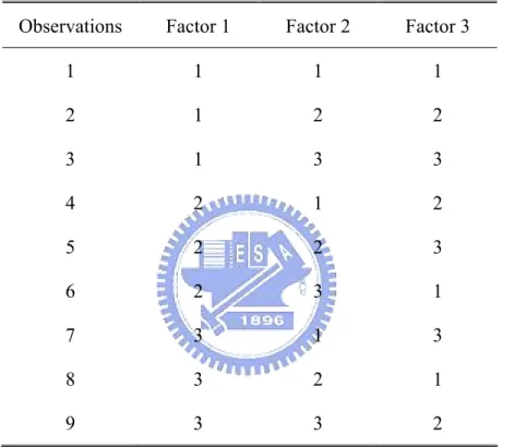
Table I. Orthogonal array L9 (33) includes 3 factors, 3 levels in each factor and 9

observations in Taguchi method………...……….36 Table II. First experimental results included of sensitivity, bandwidth, fitness

function and optimized parameters with orthogonal array L9 (33) are

calculated by Taguchi method………..….37 Table III. Second experimental results included of sensitivity, bandwidth, fitness

function and optimized parameters with orthogonal array L9 (33) are

calculated by Taguchi method………...…38 Table IV. Third experimental results included of sensitivity, bandwidth, fitness

function and optimized parameters with orthogonal array L9 (33) are

calculated by Taguchi method………..….39 Table V. Fourth experimental results included of sensitivity, bandwidth, fitness

function and optimized parameters with orthogonal array L9 (33) are

calculated by Taguchi method………...40 Table VI. The optimized diaphragm length, diaphragm thickness, air gap height,

sensitivity and bandwidth in original, Taguchi method, GA and GA with constrained bandwidth at 16, 20, 30 and 40 kHz……….….41 Table VII. Lagrange interpolation FIR filter coefficients for N =1 and N =2….42

Table VIII. The SNRs and SNR gains of one and four microphones measured by a MEMS microphone array with a 15 mm aperture and a conventional microphone array with a 12 cm aperture………..………….43

LIST OF FIGURES

Figure 1. The cross-sectional view of a single MEMS condenser microphone with a diaphragm, an air gap, a perforated backplate and a back chamber…..….44 Figure 2. The equivalent circuit based on the electro-acoustical analogy of the

condenser microphone. (a) Complete system composed of three coupled sub-systems: the acoustical system, mechanical system and electrical system. (b) Detailed circuit representation of the acoustical subsystem…45 Figure 3. The MATLAB Graphical User Interface (GUI) is utilized to change the

parameters of the linear dynamic model of the MEMS condenser microphone.………..…..46 Figure 4. The parameters optimized by GA with constrained bandwidth at 30 kHz.

(a) Optimal diaphragm length (b) Optimal diaphragm thickness………...47 Figure 5. The parameters optimized by GA with constrained bandwidth at 30 kHz.

(a) Optimal air gap height (b) Optimal frequency response………...……48 Figure 6. The comparisons of frequency responses. (a) GA , Taguchi method and

original (b) GA with constrained bandwidth at 16, 20, 30 and 40 kHz and original……….……...……49 Figure 7. The fabrication process flow of a MEMS diaphragm (a) - (i)………...….50 Figure 8. The MEMS diaphragm fabrication after anisotropic etching by KOH 30％ at 80℃………....51 Figure 9. The fabrication process flow of a MEMS condenser microphone

(a)–(q)………..…52,53 Figure 10. The configuration of an uniform linear array (ULA). A point source is

located at the far-field……….54 Figure 11. The schemes of ULAs. (a) A broadside array (b) An endfire array…...….55

Figure 12. The relationship between noise sensitivity and directivity index. (a) A broadside array (b) An endfire array……….……56

Figure 13. The comparisons of directivity index with changing factor ε in 0, 0.1, 0.01 and 0.001 using superdirective method. (a) A broadside array (b) An endfire array………..……….57 Figure 14. The comparisons of white noise gain with changing factorε in 0, 0.1, 0.01

and 0.001 using superdirective method. (a) A broadside array (b) An endfire array………...……58

Figure 15. The comparisons of optimum weight with changing factor ε in 0, 0.1,

0.01 and 0.001 using superdirective method. (a) A broadside array (b) An endfire array……….……….……….59

Figure 16. The comparisons of directivity index of delay-sum and superdirective with ε = 0.01. (a) A broadside array (b) An endfire array...60 Figure 17. The comparisons of white noise gain of delay-sum and superdirective with ε = 0.01. (a) A broadside array (b) An endfire array………..……..61 Figure 18. The comparisons of optimum weight of delay-sum and superdirective with ε = 0.01. (a) A broadside array (b) An endfire array………62 Figure 19. The comparisons of optimum weight of delay-sum and superdirective with ε = 0.01. (a) A broadside array (b) An endfire array………..…..63 Figure 20. The contour plots in an endfire array. (a) Delay-sum (b) Superdirective...64 Figure 21. The non-causal impulse response of superdirective FIR filters of order 64. (a) Microphone 1 (b) Microphone 2 (c) Microphone 3 (d) Microphone 4……….….65 Figure 22. The causal impulse response of superdirective FIR filters of order 64.

(a) Microphone 1 (b) Microphone 2 (c) Microphone 3 (d) Microphone 4………..66 Figure 23. The comparisons of the DOA estimation by delay-sum and superdirective methods with a single frequency at 500 Hz. The sound source is located at

o

10 . (a) Simulations (b) Measurements………...…..67 Figure 24. The comparisons of the DOA estimation by delay-sum and superdirective methods with a single frequency at 1000 Hz. The sound source is located

at _{10 . (a) Simulations (b) Measurements………...……..68} o

Figure 25. The comparisons of the DOA estimation by delay-sum and superdirective methods with a single frequency at 2000 Hz. The sound source is located

at _{10 . (a) Simulations (b) Measurements………...…..69} o

Figure 26. The comparisons of the DOA estimation by delay-sum and superdirective methods with a single frequency at 4000 Hz. The sound source is located

at _{10 . (a) Simulations (b) Measurements………...…..70} o

Figure 27. The DOA estimations are simulated by MATLAB using delay-sum and superdirective methods. The sampling frequency is 16000 Hz. The number of microphones is 4 with a 12 cm aperture………...………71 Figure 28. The configuration of a MEMS microphone array with same spacing 5 mm and a 15 mm aperture……….……72 Figure 29. The configuration of a conventional microphone array with same spacing 4 cm and a 12 cm aperture……….………73 Figure 30. The far-field radiation beam pattern of a continuous line source……...…74 Figure 31. The relationship between beamwidth and frequency of a continuous line source. (a) A 15 mm aperture (b) A 12 cm aperture……….…..75

Figure 32. The directivity of one microphone. (a) Simulations (b) Measurements….76 Figure 33. The directivity of a broadside array with four MEMS microphones with a 15 mm aperture. (a) Simulations (b)Measurements………..…….77 Figure 34. The directivity of a broadside array with four conventional microphones with in a 12 cm aperture. (a) Simulations (b) Measurements………78 Figure 35. A 4×4 sub-array microphones scheme……….……..79 Figure 36. The directivity of 4×4 sub-array. (a) Aperture size is 12 cm (b) Aperture size is 15 cm……….…..80

Figure 37. An HRTF example of KEMAR at elevation =_{0 and azimuth =}o _{40 .} o

(a) The HRTF frequency response (b) The impulse response (HRIR)…..81 Figure 38. The contour plots of beamforming techniques by inverse filters at 500 Hz. The source is indicated on the plot. (a) Aperture size is 15 mm (b) Aperture size is 12 cm……….…..82 Figure 39. The contour plots of beamforming techniques by inverse filters at 1000 Hz.

The source is indicated on the plot. (a) Aperture size is 15 mm (b) Aperture size is 12 cm………..…….83 Figure 40. The contour plots of beamforming techniques by inverse filters at 2000 Hz.

The source is indicated on the plot. (a) Aperture size is 15 mm (b) Aperture size is 12 cm……….……..84 Figure 41. The contour plots of beamforming techniques by inverse filters at 4000 Hz.

The source is indicated on the plot. (a) Aperture size is 15 mm (b) Aperture size is 12 cm………..….85 Figure 42. The system block diagram of 3D spatial sound reconstruction with HRTF implemented by TMS320C3X DSP………...…86 Figure 43. The implementation of a MEMS microphone array with a 15 mm

aperture……….…..87 Figure 44. The implementation of a conventional microphone array with a 12 cm

aperture………...……88 Figure 45. The implementation of the circuits with amplifiers and two second-order low pass filters……….……….…………..……89 Figure 46. The flow chart of 3D spatial sound reconstruction with HRTF…….……90 Figure 47. The DOA estimation of the delay-sum and superdirective methods, where a sound source is located at _{10 measured by the microphone array and} o

calculated by TMS320C3X DSP………91 Figure 48. The relationships of delay sample and beamforming angle with sampling rate at 8, 16, 25 and 50 kHz……….…………..…….92 Figure 49. The results of listening test of the 3D spatial sound reconstruction with

Figure 50. The perceived angle errors at the presented angle of listening test of the 3D spatial sound reconstruction with HRTF implemented by TMS320C3X DSP………...…..94

I. INTRODUCTION

A microphone is a transducer, which transforms acoustical energy to electrical energy and can be fabricated by Micro-Electro-Mechanical System (MEMS) technology.1 The types of microphone consists of piezoelectric,2 piezoresistive3 and capacitive4-10. Among them, the performance of the capacitive microphone is best because of its high sensitivity, flat frequency response and low noise level. The advantages of the MEMS technology are the small size and better performance. However, the fabrication of micromachining induces a large initial stress in the diaphragm. The large initial stress of the diaphragm degrades the performance of the condenser microphone. Therefore, how to decrease the initial stress of the diaphragm is an important problem. The material of diaphragm should be chosen carefully.

The linear dynamic model of the MEMS condenser microphone is introduced.11-13 Therefore, the dynamic performances can be acquired. In order to maximize the performances of the MEMS condenser microphone, Taguchi method14,15

and Genetic Algorithm (GA)16,17 are presented. The performances of the MEMS

condenser microphone consist of sensitivity and bandwidth. We expect the sensitivity and bandwidth as larger as possible, but the relationship between them is trade-off. Therefore, Taguchi method and GA are utilized to optimize the values of the sensitivity and bandwidth. The parameters that need to be optimized are diaphragm length, diaphragm thickness and air gap height. From the results of optimization, sensitivity and bandwidth are improved, respectively. After optimization, the optimal parameters are acquired. Therefore, the processes of the microphone diaphragm can be designed and fabricated using the MEMS technology. The purpose to fabricate the microphone diaphragm is to know the resonant frequency in the diaphragm. Then, the initial stress of the diaphragm can be acquired and the

sensitivity of the diaphragm can be controlled. In addition, Poly-Silicon is used for diaphragm material to degrade the initial stress. On the other hand, the processes of the MEMS condenser microphone structures are also designed with a single silicon wafer. The fabrication is not done, just in design steps.

Array signal processing18-20 has been widely used in the areas such as radars, sonars, communications, and seismic exploration, and underwater imaging. The major advantage is the enhancement of the Signal-to-Noise Ratio (SNR). Besides, the directivity of the microphone array can be improved to be effective in eliminating background noise by beamforming techniques. Array signal processing of Direction of Arrival (DOA) estimation and beamforming techniques are utilized. The delay-sum and superdirective methods are utilized to do the DOA estimation and beamforming. The locations of the sound source can be estimated. Then, a microphone array can point to the direction of source to receive signals. Therefore, SNR and directivity can be improved greatly.

In order to reconstruct three-dimensional (3D) spatial sound field, the

microphone array with Head Related Transfer Function (HRTF)21 are utilized to

realize our goal. Most hearing-impaired people will be able to hear speech when given sufficient amplification from their hearing aids. However, they will hear but will not understand because of poor SNR. In a noisy place, hearing aids will amplify the noise as well as the desired speech signal. In a reverberant place, hearing aids will amplify late reverberation as well as the direct first arrival signal. Furthermore, acoustical feedback also degrades the SNR and distorts the frequency response of the hearing aids. The microphone array for hearing aids can enhance SNR. Besides, it can reduce the effects of reverberation and acoustical feedback. The microphone array is worn on the chest as part of a necklace to receive the sound source. The filters between the microphone array and hearing-impaired people’s ears can be

calculated by sound propagation transfer function and HRTF. The inverse filters can be implemented to reconstruct 3D spatial sound field. Then signals received by the microphone array do the DOA estimation to find the location of the sound source. Therefore, the 3D spatial sound can be reconstructed with a microphone array using HRTF. Therefore, the hearing-impaired people can hear the spatial sound in three-dimensional space. The aforementioned advantages are also included.

II. MEMS CONDENSER MICROPHONES

Most of the silicon microphones presented in the literature are based on the capacitive principles because of its high sensitivity, flat frequency response and low noise level. The capacitive microphone consists of a thin, flexible diaphragm and a rigid backplate. Mechanical sensitivity is mainly determined by the initial stress and Young’s modulus of the diaphragm. Large initial stress and Young’s modulus in the diaphragm can seriously degrade the sensitivity of the condenser microphones. In order to improve the sensitivity, low-stress Poly-Silicon is used as the diaphragm

material.22 First, linear dynamic model of a condenser microphone needs to be

constructed. Then, dynamic performance of frequency response, sensitivity and bandwidth of a condenser microphone can be acquired. After this, Taguchi method and GA are used to maximize the sensitivity and bandwidth of a condenser microphone. The scales of diaphragm length, diaphragm thickness and air gap height of a condenser microphone can be optimized. Therefore, the performances of a MEMS condenser microphone can be improved.

A. The Linear Dynamic Model

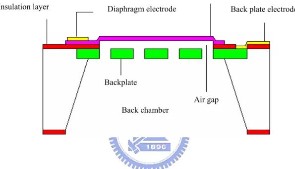
Figure 1 shows the cross-sectional view of a single MEMS condenser microphone with a diaphragm, an air gap, a perforated backplate and a back chamber.

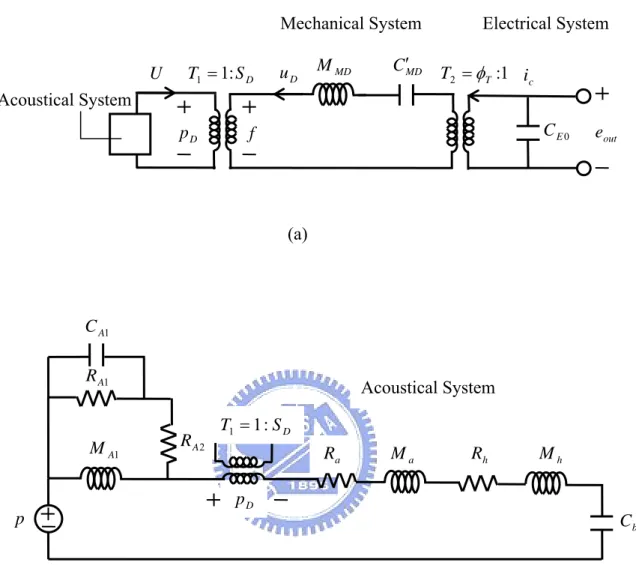
When a surrounding acoustic pressure is applied, a pressure difference appears in the back chamber and causes the diaphragm to deflect. The deflection of the diaphragm is measured as a change of electrical capacitance between the diaphragm and the perforated backplate. Then the changes of electrical capacitance are the received signals of the microphone. Assume that backplate is rigid and deflection is small so that the linear model applies. Electro-acoustical analogy is adopted for predicting the linear dynamic behavior of the MEMS condenser microphone. The equivalent circuits of the microphone are shown in Figure 2, wherein the acoustical, mechanical and electrical domains are coupled through ideal transformers. The acoustical system consists of resistance and mass due to radiation from the diaphragm, the air film in the air gap and the air in the acoustic holes in the backplate, and compliance of the air in the back chamber. The mechanical system consists of compliance and mass of the diaphragm and the backplate. Figure 3 shows the MATLAB Graphical User Interface(GUI). The MATLAB GUI is utilized to change the parameters of the linear dynamic model of the MEMS condenser microphone. Then the frequency response of the MEMS condenser microphone can be acquired. After linear dynamic model, the optimal design of the performances for the MEMS condenser microphone is following.

B. Optimal Microphone Design

In order to improve the performance of a condenser microphone, Taguchi method and GA is utilized to optimize the main parameters of diaphragm length, diaphragm thickness and air gap height. Then the performance indices of sensitivity and bandwidth can be improved.

1. Taguchi Method

World War and is an experimental design procedure for examining multi-factors in a design problem using a minimum number of observations.14,15 In fact, it is the most powerful method available to reduce product cost, improve quality, and simultaneously reduce development interval. A general Taguchi procedure provides three kinds of functions: system design, parameter design and tolerance design. For our problem, we focus primarily on parameter design. Parameter design uses the orthogonal array to compute the optimal solution. The orthogonal array is composed of factors and levels and it can reduce the computation load. Factor is the parameter that needs to be optimized. Level is the value of each factor. The simplified procedures of parameter design by Taguchi method have 5 steps. First, choose the factors that need to be optimized. Second, choose the fitness function. Third, choose the levels of every factor. Fourth, use the orthogonal array to compute the optimal level of every factor. Fifth, repeat third and fourth step until find the optimal solutions.

In our problem, we wish to maximize the sensitivity and bandwidth of a MEMS condenser microphone. First, parameters that need to be optimized are diaphragm length(DL), diaphragm thickness(DT) and air gap height(AH). Other parameters in the MEMS microphone model do not greatly affect the performances. Second, fitness function f is chosen

3 4 1 0.4 10 10 f S BW − = × × + × (1)

where S and BW are the sensitivity and bandwidth of the MEMS condenser

microphone. Third, three levels of every factor are chosen. Fourth, a L9 (33)

orthogonal array is chosen and shown in Table I, where ‘1’ represents the first level of a factor, ‘2’ represents the second level of a factor, ‘3’ represents the third level of a

observations, 3 factors and each factor has 3 levels. The larger values of fitness function have better performances. Taguchi method is done by four times experiments to find the optimal solutions. Tables II-V are the results of four times experiments. The optimal solutions of diaphragm length, diaphragm thickness and air gap height by Taguchi method are 1.1 mm, 1.6 µm and 2.2 µm. The sensitivity and bandwidth of the MEMS condenser microphone are 7.7 mV/Pa and 18.38 kHz. Sensitivity is improved by Taguchi method but bandwidth is somewhat degraded. 2. Genetic Algorithm

Genetic Algorithm(GA) is a search algorithm based on the natural selection, genetics and evolution.16,17 It is also a stochastic and powerful method for solving optimization problems. GA was first published by Holland in 1962. It has proven to be efficient in many areas such as function optimization and image processing. It is composed of the procedures of encoding, decoding, fitness function, reproduction, crossover and mutation. The simplified procedures of optimization by GA have 5 steps. First, choose the parameters needed to be optimized. Second, choose the fitness function. Third, choose the upper limit, lower limit and resolution of every parameter. Fourth, do encoding, decoding, reproduction, crossover and mutation for every generation. Fifth, repeat fourth step until find the optimal solutions. In the following, GA is introduced in details.

For encoding and decoding, all processes of GA are operated with binary strings encoded from original parameters. The resolution of a parameter space is dependent on the amount of bits per string and searching domain of the parameter. The resolution can be obtained as follows

2 1 i i U L i i x l x x R = − − (2) where U i x and L i

the parameter range is 0 ＜ x ＜ 5.5 cm. Then the number of bits needed for x is assumed 8. Therefore, the desired resolution is R = 0.0216. If parameter x is 2.592, _x

then the value after encoding is [ 0 1 1 1 1 0 0 0 ]. Fitness function is the performance index for GA and chosen same as Taguchi method in Eq. (1).

Reproduction is a rule of survival of fittest. The larger value of fitness function of the factors in every generation, the higher reproduction probability can be generated. The reproduction probability S is shown as i

1 i l c i P c k f S f = =

∑

(3) where i c

f is the fitness function of the i factor, P is the population size. For _l

instance, there are four factors, c₁~ c₄, in the zero generation with fitness functions

40, 5, 72 and 54. By substituting those values into Eq. (3), the reproduction probabilities are S₁=0.2239 , S₂ =0.0292 , S₃ =0.4211 and S₄ =0.3158 ,

respectively. The factors c and ₃ c₄ have the large probability to reproduce in the

next generation. Next, in the present population, four random numbers between 0 and 1 are generated. For example, if the four random numbers are 0.3675, 0.8719, 0.7697 and 0.1437, the factors of next generation will be c ,₃ c₄ ,c₄ and c₁,

respectively.

Crossover is exchange the information of the factors. First, the crossover ratio

r

C is defined (in general, 0.8≤C_r ≤1 and we choose C_r =0.85) and two factors in

the present population are selected randomly. Second, a random number is selected to check whether crossover or not. If the random number is larger than crossover ratio, then crossover needs to be done. The factors codes after the chosen point are interchanged. If the random number is less than crossover ratio, then the original factors is still the next generation. To illustrate, there are two factors c₁ and c₂

with the chosen point at third bit: c₁ =011∆0111, c2 =101∆1001. With crossover,

two new factors are generated: ~c₁ =011_∆1001, c~₂ =101_∆0111.

However, the optimal solutions in GA may be local optimal solutions. To overcome this problem, mutation is introduced into the GA procedure. Let the mutation ratio be M_r (in general, 0≤M_r ≤0.01 and we choose M_r =0.01).

Choose a random number to determine whether mutation or not and choose mutation

point. .For example, a factor c₁ with the mutation point at third bit is

10100 1 10

1 = _∆

c . After mutation, the factor becomes ~₁ 10010100

∆

=

c . The

mutation rate can not be chosen too large, or the search will be unhelpful.

In our problem, the search range of diaphragm length, diaphragm thickness and air gap height are 7-1.5 mm, 0.8-2.5 µm and 2.0-4.0 µm. The number of bits is 12. The crossover rate is 0.85. The mutation rate is 0.01. The computed generation is 150. The optimized values of diaphragm length, diaphragm thickness and air gap height are 1.0252 mm, 2.1362 µm and 2.1084 µm. In order to realize in MEMS scale, the parameters need to be chosen to minimum in MEMS process technology. Therefore, the parameters are chosen as 1.02 mm, 2.1 µm and 2.1 µm. The performances computed by GA with fitness function in Eq. (1) are 5.4 mV/Pa and 24.6 kHz. The sensitivity is too small. The reason maybe the fitness function is too simplified, because the relationship of sensitivity and bandwidth is not linear. The exact fitness function is not easy to get because there are three parameters that need to be optimized.

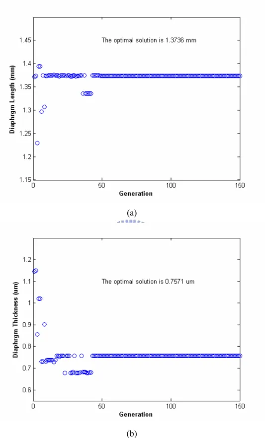
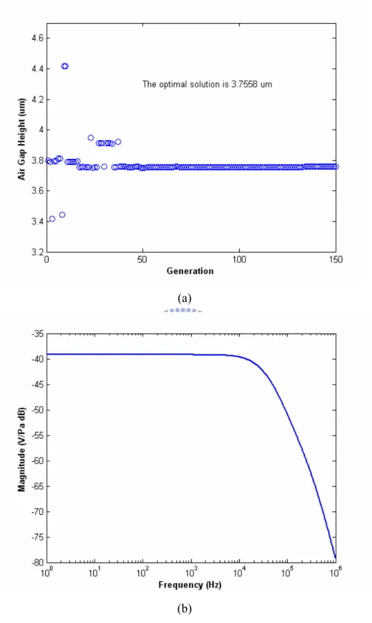
Then, fix the bandwidth over a range. The fitness function is sensitivity only. Figure 4 shows the optimized values of diaphragm length and diaphragm thickness using GA with constrained bandwidth at 30 kHz. Figure 5 shows the optimized values of air gap height using GA with constrained bandwidth at 30 kHz and the

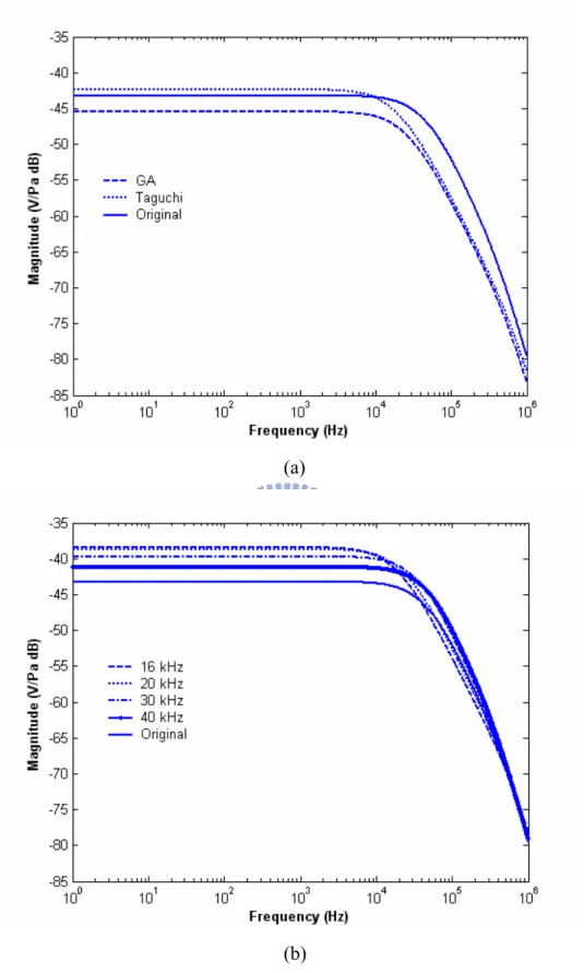
frequency response. The optimized sensitivity and bandwidth are 10.3 mV/Pa and 33.3 kHz. The sensitivity is improved greatly. Three optimized values are 1.24 mm, 0.8 µm and 3.4 µm. The comparisons of frequency response of Taguchi method, GA, GA with constrained bandwidth at 16, 20, 30 and 40 kHz are shown in Figure 6. Table VI shows diaphragm length, diaphragm thickness, air gap height, sensitivity bandwidth of original, GA, Taguchi method, GA with constrained bandwidth at 16, 20, 30 and 40 kHz. From the results, the performances of the MEMS condenser microphone can be improved greatly.

C. MEMS Diaphragm Process Design and Fabrication

The initial stress greatly affects the sensitivity of a MEMS condenser microphone. In order to know the real value of initial stress in the diaphragm, we have to design and fabricate a MEMS diaphragm with Poly-Silicon. The thickness of the diaphragm is 1 µm and the lengths of the diaphragm are designed for 1, 1.2, 1.4, 1.6, 1.8 and 2.0 mm. Different lengths of the diaphragm can be caused different resonant frequencies. Then, we can know the value of initial stress in the diaphragm to control the sensitivity of the diaphragm. By the way, the resonant frequency of the diaphragm can be calculated by13

1 2 r D D f M C π = (4)

where M and D C is mass and compliance of the diaphragm, respectively. The D

imaginary part of the impedance determines the resonant frequency of the diaphragm. The real part of the impedance determines the damping effects of the diaphragm. From the frequency response of the dynamic model of the condenser microphone, the 3 dB down cut-off frequency is 42.5 kHz. The real resonant frequency of the microphone computed by Eq. (4) is 105 kHz, not 42.5 kHz. This is because that the

real part of acoustical impedance is large enough to oppress the resonant frequency. Therefore, the resonant frequency of the linear dynamic model of the MEMS condenser microphone can not be shown. The effects of real and imaginary parts of the impedance should be greatly realized.

The fabrication procedures of the MEMS diaphragm are shown in Figure 7. The diaphragm is square. The silicon wafer we used is N-type, <1 0 0> crystal structure, 525 µm thick, and resistivity is 1~10 Ωcm. The Si3N4 is deposited for

5000 Ǻm thick as resistant layer using LPCVD at 800℃. This layer is to resist the KOH etching and protect the bottom side of the diaphragm. The low-stress Poly-Silicon is deposited for 1 µm thick as diaphragm structure using LPCVD at 620 ℃. This layer is the main structure of the condenser microphone. The acoustic waves can be detected by the diaphragm. The Si3N4 is deposited for 5000 Ǻm as

resistant layer using LPCVD at 800℃. This layer is also to resist the KOH etching and protect the top side of the diaphragm.

After all the layers are deposited, we should pattern the back chamber holes to realize the diaphragm structure. Then, RIE is used to pattern the back chamber holes of the bottom side of the wafer. The back chambers are formed by use of anisotropic etching in a KOH 30% solution at the temperature of 80℃. After etching, the Si3N4

layer is released by HF. Therefore, the diaphragm structure is realized. Figure 8 shows the result of the diaphragm anisotropic etching by KOH. We know that each diaphragm is etched quite square but the thickness is not very flat. The average thickness measured by surface profiler is 60 µm. Some diaphragms are etched broken and some still have 60 µm thick. The reasons are due to the etching rate of KOH is not uniform and the layers deposited are not very flat. In addition, the resistant layer of Si3N4 is too thin to resist the KOH. Therefore, some diaphragms

D. MEMS Microphone Process Design

The fabrication steps of a MEMS condenser microphone are shown in Figure 9. The silicon wafer we used is N-type, <1 0 0> crystal structure, 525 µm thick, and resistivity is 1~10 Ωcm. The SiO2 is deposited for 2000 Ǻm thick as resistant layer

to pattern the boron diffusion area as backplate using wet oxidation. Diffuse the boron in the silicon wafer and remove the SiO2 using BOE. The Si3N4 is deposited

for 2500 Ǻm as insulation layer to pattern the diaphragm area and backplate electrode area using LPCVD. The SiO2 is deposited for 3 µm thick as sacrificial layer to

define the air gap height using wet oxidation. Pattern the 3 µm thick SiO2 for

diaphragm area. The Poly-Silicon is deposited for 1 µm thick as diaphragm using LPCVD. Pattern the 1 µm thick Poly-Silicon for proper diaphragm area and show

the backplate electrode contact pad. The SiO2 is deposited for 1 µm thick as

insulation layer using wet oxidation. Pattern the SiO2 and Si3N4 to define the back

chamber size. The back chamber holes are formed by use of anisotropic etching in a

KOH 30% solution at the temperature of 80℃. Remove the 3 µm thick SiO2 to

release the air gap. Deposit Cr for 50 nm as adhesion layer and Au for 400 nm as electrode by evaporation. Then, pattern diaphragm contact pad and backplate contact pad and remove Cr in HNO3+NH4F and Au in KI.

III. MICROPHONE ARRAY SIGNAL PROCESSING

Array signal processing techniques are utilized for Direction of Arrival (DOA) estimation and beamforming. There is a one important thing we have to know. Avoid spatial aliasing or grating lobes, the spacing between each microphone must be less than half wavelength of the signals. In the following array signal processing, we assume that signals received at reference point are far-field and narrowband. Far-field assumes that the signals are located far enough away from the array that the

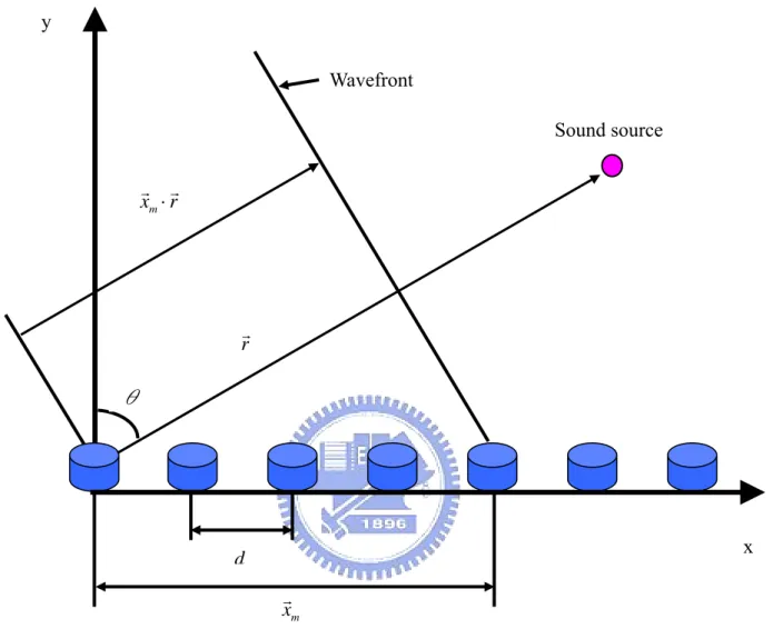
wavefronts impinging on the array can be modeled as plane waves. On the other hand, the effects of distance on field intensity can be neglected. Narrowband assumes that the incident signal that the Beamformer is trying to capture has a narrow bandwidth centered at a particular frequency. The uniform linear array (ULA) is shown in Figure 10 and the array model can be constructed.

A. Direction of Arrival (DOA) estimation and Beamforming

DOA estimation and beamforming of speech signals using a set of spatially separated microphones in an array has many practical applications such as video-conferencing system and hearing-aids. The locations of sound source can be found out by the DOA estimation. The beam of the array can be moved to the sound source to receive the signals is a beamforming technique. Two types of linear arrays with equally spaced microphones are discussed. Figure 11 shows the configuration of the broadside and endfire arrays. A “broadside” array has its microphones along a line perpendicular to the sound direction and an “endfire” array has its microphones along a line collinear with the sound direction.

1. The Delay-Sum Method

The spacing between adjacent microphones is d. Assume that the signal r(t)

at a reference point is a narrowband with center frequency ωc:

( ) ( ) j ct

r t =s t eω (5)

where )s(t is the phasor of r(t). The signal received at the mth array element

located at xr is denoted as _m x_m(t), and let rr be the unit vector pointing to the

sound source direction. If the speed of sound is c, the signal x_m(t) can be written

as ) ( ) ( ) ( ) ( ) ( e e n t c r x t s t n c r x t r t x c j t _m r x j m m m m c m c + ⋅ + = + ⋅ + = ω ⋅ ω r r r r r r (6)

where )n_m(t is the noise signal of the mth component in the array. In general, ) ( ) ( s t c r x t s + m⋅ ≈ r r

for far field approximation. For M sensor signals

) ( , ), ( 1 t x t

x L M , the data vector can be formed as

) ( ) ( ) ( ) ( ) ( ) ( ) ( ) ( ) ( 1 1 1 t t r r t n t n e t s e e t x t x t M t j c r x j c r x j M c M c c n a x = + ⎥ ⎥ ⎥ ⎦ ⎤ ⎢ ⎢ ⎢ ⎣ ⎡ + ⎥ ⎥ ⎥ ⎥ ⎥ ⎦ ⎤ ⎢ ⎢ ⎢ ⎢ ⎢ ⎣ ⎡ = ⎥ ⎥ ⎥ ⎦ ⎤ ⎢ ⎢ ⎢ ⎣ ⎡ = ⋅ ⋅ r M M M r r r r ω ω ω (7)

where )a(rr is called the array manifold vector. The unit vector rv for a sound source at the θ direction is given by

) cos , (sinθ θ = rr (8)

The position vector of the mth element can be expressed as

) 0 , ) 1 ((i d xr_m = − (9)

Then the inner product of the position vector and the unit vector is obtained

θ sin ) 1 (i d r xr_m⋅ r= − (10)

The array manifold vector a(rr) can be rewritten from Eq. (10)

T c d M j c d j c c c e e _⎥ ⎦ ⎤ ⎢ ⎣ ⎡ = ω θ ω − θ θ ω , ) 1 sin ( 1) sin ( _L a (11)

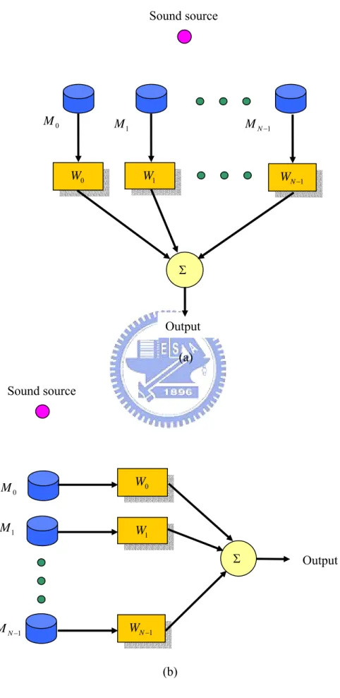
Extension from the narrowband formulation to the broadband formulation is straightforward. The center frequency ω_c is replaced by ω , where ω means a broadband frequency variable. The beamformer output y(t) is the weighted sum of the delayed input signals x_m(t),m=1_LM ,

) ( ) ( 1 0 kT t x w t y _m M m N k mk − =

∑∑

= = (12)

Equation (12) can be rewritten in the frequency domain for a particular direction θ as )) ( ) ( ) , ( )( ( ) , ( ) ( ) , (ω θ =h e ω x ω θ =h e ω a ω θ r ω +n ω y j j (13)

T c d M j c d j e e _⎥ ⎦ ⎤ ⎢ ⎣ ⎡ = ω θ ω − θ θ ω, ) 1 sin ( 1) sin ( _L a (14) and ( ω) [ ₁( ω) ₂( ω) ( jω)] M j j j e h e h e h e = _L

h is consisted of Discrete Time Fourier

Transforms (DTFT) of each tapped-delay line channel. The frequency response is given by

∑

= − = N k kT j mk j m e w e h 0 ) ( ω ω , m=1_LM (15)

N and T are the filter order and the sampling period, respectively. The

dimensions of ( jω)

e

h and a(ω,θ) are 1×M and M ×1, respectively.

In our problem, the delay-sum algorithm is tried to find ( jω)

e

h that maximizes

signal-to-noise ratio gain (SNRG), i.e. ) ( ) ( ) ( ) ( ) ( ) ( max ) ( ω ω ω ω ω θ θ j H j j H H j e e e e h h h a a h h (16) which is equivalent to 1 ) ( ) ( to suject ) ( ) ( ) ( ) ( max ) ( = ω ω ω ω ω θ θ j H j j H H j e e e e a a h h h h h (17)

This problem can be solved by Lagrange multiplier method, the solution is obtained as below ) , ( ) ( jω H ω θ e a h = (18)

Equation (17) explains that each channel filter equals to the conjugate of each component in the manifold vector.

M m e e e h c j m d m j j m( ) , 1L sin ) 1 ( = = = −ω − θ −ωτ ω _{, (19)} where c d m m θ

τ = ( −1) sin is the delay of each channel according to the difference

between mth sensor and reference point. However, the delay usually is not an

integer in the digital processing. There are many ways to deal with these fractional delay problems. The simplest approach is Lagrange interpolation method. Firstly we divide τ_m by sampling period T to acquire the fractional delay Ψ . The _m

delay is separated into two parts m m m m e D T =Ψ = + τ (20) where D and _m e are the integer and fractional component of _m Ψ , respectively. _m

For simplicity, the Finite Impulse Response (FIR) filter coefficients are obtained from Eq. (21) to realize the Lagrange interpolation.

N k l k l e w m N k l l mk , 0,1,2K 0 − = − ∏ = ≠ = (21)

The coefficients for the Lagrange filters of order N =1, 2 are given in the Table VII. The case N =1 corresponds to linear interpolation between two samples. Once we

obtain the filters, the output signals y(ω,θ) can be calculated from Eq. (13). The square of y(ω,θ) is called the spatial power spectrum, which is given by

) ( ) , ( ) , ( ) ( ) , ( ) (θ ω θ 2 jω ω θ H ω θ H jω e e y S = = h x x h (22)

The maximum magnitude of the spatial power spectrum is the direction of the sound source.

2. The Superdirective Method

The superdirective method is presented.23-28 From the delay-sum method, we can know that signals which got from microphones are

( j ) ( j ) ( j )

s

eω = eω + eω

x s d v (23)

where d is the look direction vector which depends on the actual geometry of the _s array and the direction of the sound source signal. Then, the output is

H

y = w x (24)

where w denotes the frequency-domain coefficients of the beamformer and the

operator H _{denotes a complex conjugated transposition (Hermitian operator). The}

array gain is the measure which shows the improvement of the SNR between one sensor and the output of the whole array. Therefore,

Array Sensor SNR G SNR = (25)

The SNR of one sensor is given by the ratio of the power spectral densities (PSD) of the signal φ_ss and the average noise

a a

V V

φ . The SNR at the output can be computed by deriving the PSD of the output signal.

H YY = XX φ w φ w (26) where 0 0 0 1 0 1 1 0 1 1 1 1 1 0 1 1 1 1 N N N N N N X X X X X X X X X X X X XX X X X X X X φ φ φ φ φ φ φ φ φ − − − − − − ⎛ ⎞ ⎜ ⎟ ⎜ ⎟ = ⎜ ⎟ ⎜ ⎟ ⎜ ⎟ ⎜ ⎟ ⎝ ⎠ φ K K M M O M K

is a power spectral density matrix of

the array input signals. When the desired signal is present only, the output is

2

H YY _Signal = SS s

φ φ w d (27)

and for noise only case the output is

a a

H YY Noise =φV V V V

φ w φ w (28)

where φVV is a normalized cross power spectral density matrix of the noise.

Therefore, array gain in Eq. (25) can be rewritten as

2 H s H VV G= w d w φ w (29)

Assuming a homogeneous noise field can be expressed in terms of the coherence matrix 0 1 0 2 0 1 1 0 1 2 1 1 2 0 2 1 2 1 1 0 1 1 1 2 1 1 1 1 N N N N N N V V V V V V V V V V V V V V V V V V VV V V V V V V − − − − − − Γ Γ Γ ⎛ ⎞ ⎜ ⎟ Γ Γ Γ ⎜ ⎟ ⎜ _{Γ Γ Γ} ⎟ = ⎜ ⎟ ⎜ ⎟ ⎜ ⎟ ⎜ ⎟ ⎜_{Γ Γ Γ} ⎟ ⎝ ⎠ Γ K K K M M M O M K (30) where ( ) ( ) ( ) ( ) n m n m n n m m jw V V jw V V _{jw jw} V V V V e e e e φ Γ =

gain can be rewritten again as 2 H s H VV G= w d w Γ w (31)

This representation allows for different noise fields and they can be expressed by their coherence function.

A common quantity to evaluate beamformers is the directivity index (DI) which describes the ability of the array to suppress a diffuse noise field. Therefore, we can compute the DI by using the coherence function of a diffuse noise field

[

]

sin ( ) ( ) ( ) n m jw V V _Diffuse k n m d e k n m d − Γ = − (32)

Then, directivity index (DI) is

2 10 10log ( ) H s H VV Diffuse DI = w d w Γ w (33)

The ability of the array to suppress spatially uncorrelated noise, which can be caused by self-noises of the sensors. Inserting the coherence matrix for this noise field

VV uncorr =

Γ I (34)

into Eg. (30) results in the white noise gain (WNG)

2 H s H WNG= w d w w (35)

On a logarithmic scale positive values represent an attenuation of uncorrelated noise, whereas negative values show an amplification.

In the real implementation of superdirective beamforming, large microphone weights result in array instability and sensitivity to uncorrelated noise. The noise sensitivity ( )Ψ 26

* H T H s s Ψ = w w w d d w (36)

can be implied to illustrate the uncorrelated relationship between signals and noises.

When w is determined by Eq. (38), T 1

s =

w d , and Ψ is simply H _{| |}2

i wi

= Σ

w w .

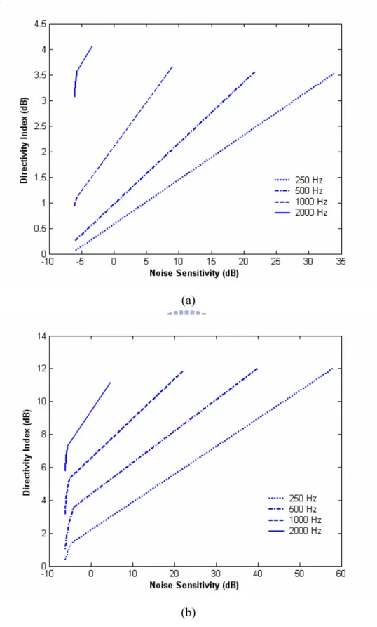
Insure that the array has unity gain in the sound source, w must be normalized to the sound source. Figure 12 shows the relationship between noise sensitivity and DI in broadside and endfire arrays. From the results, high noise sensitivity implies the larger microphone weights. In low frequencies, the optimal weights used for implementations are larger than high ones. In order to achieve the same DI, microphone weights utilized in low frequency are larger than high ones. Therefore, the DI in low frequency is hard to improve, unless the large weights are utilized.

In order to design optimal beamformers, we have to minimize the power of the output signal of the array. Avoiding the trivial solution w= 0, the minimization is constrained to give an undistorted signal response in the desired look direction. Therefore, the following constrained minimization problem has to be solved:

min H subject to H 1

XX s =

W w φ w w d (37)

Since we are only interested in the optimal suppression of the noise, and we assume a perfect correspondence between the direction of the desired signal and the look

direction of the array, only the noise PSD-matrix φ is used. The well-know VV

solution for Eq. (37) is called the Minimum Variance Distortionless Response (MVDR) beamformer.23 It is given by 1 1 VV s H s VV s − − = φ d w d φ d (38)

and can be derived by using the Lagrange-multiplier.29 Assuming a homogeneous

noise field the solution is a function of the coherence matrix:

1 1 VV s H s VV s − − = Γ d w d Γ d (39)

Eq. (36) or Eq. (37) can be interpreted as a spatial decorrelation process followed by a matched filter for the desired signal. The normalization in the denominator leads to unity signal response for the look direction.

The well-known delay-sum beamformer is included for comparison purposes. It is an “optimal” beamformer for optimizing the WNG. We can derive the coefficients from Eq. (37) by inserting the coherence matrix for spatial uncorrelated noise 1 s N = w d (40)

The WNG is optimal in this case and reaches N.

The method uses a same added scalar ε to the main diagonal of the normalized PSD or coherence matrix: 1 1 Regularized ( ) ( ) VV s H s VV s ε ε − − + = + Γ I d w d Γ I d (41)

The factor ε can vary from zero to infinity, which results in the unconstrained superdirective or the delay-sum respectively. The results between delay-sum and superdirective in broadside and endfire array are illustrated in the following.

Figure 13 shows the effects of changing factor ε in 0, 0.1, 0.01 and 0.001 for DI in the broadside and endfire arrays. From the results, we know that the DI in the endfire array is larger than the broadside array. In the broadside and endfire arrays, the DI is independent of ε above the frequencies of 2 and 3 kHz. Figure 14 shows the effects of changing factor ε in 0, 0.1, 0.01 and 0.001 for WNG in the broadside array and endfire array. From the results, we know that the WNG in the broadside array is larger than the endfire array. In the broadside and endfire arrays, the WNG

is independent of ε above the frequencies of 2 and 3 kHz. Figure 15 shows the

effects of changing factor ε in 0, 0.1, 0.01 and 0.001 for optimum weight in the broadside and endfire arrays. From the results, we know that the optimum weights

in the broadside array are larger than the endfire array. It means that the larger values of optimum weight, the harder implementations of FIR filters. In the broadside and endfire arrays, the optimum is independent of ε above the frequencies of 2 and 3 kHz. The optimal weights can not be too large, or it is hard to be implemented. The optimal weights should be small enough to implement in FIR filters. Around the effects of ε , the best values of ε is chosen as 0.01.

After the proper ε is chosen, then the comparisons of delay-sum and superdirective in DI, WNG, and optimal weights in broadside array are illustrated.

Figure 16 shows the comparisons of DI of delay-sum and superdirective with ε

chosen as 0.01 in the broadside and endfire arrays. We know that the DI with the superdirective method is improved greatly both in the broadside and endfire arrays.

Figure 17 shows the comparisons of WNG of delay-sum and superdirective with ε

chosen as 0.01 in the broadside and endfire arrays. We know that the WNG with the delay-sum method is better than the superdirective method both in the broadside and endfire arrays. Figure 18 shows the comparisons of optimum weights of delay-sum and superdirective with ε chosen as 0.01 in the broadside and endfire arrays. From the results, we know that the optimum weights with the superdirective method are larger than the delay-sum method at low frequency both in the broadside and endfire arrays. Because the WNG is small at low frequency, the optimum weights have to compensate the weights at low frequency. The weights of superdirective method can be accepted to implement as FIR filters.

In addition, the contour plots of delay-sum and superdirective methods compared in broadside array is shown in Figure 19. We know that the directivity of superdirective method in low frequency is greatly improved. It means that the SNRs of superdirective method are larger than delay-sum method. The performances of microphone can be improved by superdirective beamforming. Figure 20 shows the

contour plots of delay-sum and superdirective methods compared in endfire array. The results are still the same with the broadside array. To compare the difference of the broadside and endfire array with the performance indices indicated above, the directivity of the endfire array is better than the broadside array, but beamwidth shown in contour plots is wider than the broadside array. The reason is that the directivity is calculated from _{0 ~ 360 and the directivity of the broadside array is} o o

symmetrical at ₀o _{and 180}o _{and shown up from 0 ~ 360 . But, the directivity of} o o

endfire array is not symmetrical and shown up just from _{-90 ~ 90 . That is why} o o

the differences of directivity and beamwidth in the broadside and endfire array. Once the frequency response of the superdirective weights is obtained, the inverse Fourier transform is utilized to acquire the impulse response of the

superdirective FIR filters. If the P frequencies are acquired, the discrete _w

frequency response can be obtained as

*

( ) ( ), 1, ,

m m w

H l =w l l= L P (42)

where ( )Hm l is the discrete frequency response at mth channel and

*_{( )}

m

w l is the

discrete frequency response of superdirective algorithm at mth channel. In order to

obtain the impulse response with real coefficients, mirror H_m(l) with conjugate operation to obtain the symmetric frequency response. Then the frequency response becomes ⎪ ⎪ ⎩ ⎪⎪ ⎨ ⎧ − − − = = = = − = = ) 1 ( , , 1 ), ( ) ( , , 1 ), ( ) ( ) 1 ( ) 1 ( ) 0 ( * w m m w m m m m m P l l w l H P l l w l H H H H L L (43)

Subsequently, Eq. (43) is equivalent to shift l=−1,_L,−(P_w −1) to

1 2 , , 1 − + =Pw Pw

⎪ ⎪ ⎩ ⎪⎪ ⎨ ⎧ − + = = = = = ) 1 2 ( , , ) 1 ( ), ( ) ( , , 1 ), ( ) ( ) 1 ( ) 0 ( * w w m m w m m m m P P l l w l H P l l w l H H H L L (44)

Finally, the impulse response can be obtained by utilizing inverse Fourier transform at each channel. ) 1 2 ( 1 , ) ( 2 1 ) ( 2 1 0 2 − = =

∑

− = − w P l lk P m w m H l W k P P k h w w L (45) where w w w P j P j P e e W π π ₋ − = = 2 ) 2 (

2 . In general, hm(k) may be non-causal. The half of

) (k

h_m can be moved to center as symmetrical about the center. Figure 21 shows the

non-causal impulse response of superdirective FIR filters of order 64. The causal impulse response of superdirective FIR filters of order 64 is shown in Figure 22. Therefore, the digital superdirective FIR filters are implemented. From the results, the FIR filters are symmetrical. The superdirective FIR filters of Microphone 1 are the same with Microphone 4. The superdirective FIR filters of Microphone 2 are the same with Microphone 3. Besides, the relationship between Microphone 1 and Microphone 2 is like ’differential microphones’. Figure 23-26 show the simulations and measurements of the DOA estimation of delay-sum and superdirective methods with a single frequency at 500, 1000, 2000 and 4000 Hz, respectively. The sound

source is indicated at _{10 . From the results, the DOA estimation angle of} o

superdirective method is more precise than delay-sum at 500, 1000 and 2000 Hz. The DOA estimation is almost the same at 4000 Hz or other high frequencies. However, the sidelobes of superdirective method are larger than delay-sum. Figure 27 shows the DOA estimation simulated by delay-sum and superdirective methods with the sampling rate 16000 Hz at a 12 cm aperture in 8 kHz broadband white noise. Obviously, the beamwidth of superdirective method is smaller than the delay-sum method and the directivity is also better than delay-sum method. However, the

sidelobes of superdirective method are larger than delay-sum. We can know that the relationship between beamwidth and sidelobes is trade-off. The DOA estimation of superdirective method is more precise than delay-sum method.

B. Directivity Analysis

Directivity is a quite important performance index for microphone arrays and the aperture size of microphone arrays dominates the value of directivity. In the following simulations and measurements of directivity, the aperture sizes of microphone array are 15 mm and 12 cm and the sound source is located at _{0 . Four} o

microphones are used to line in uniform linear array. Figure 28 shows the configuration of a MEMS microphone array with same spacing 5 mm and the aperture size is 15 mm. Figure 29 shows the configuration of a conventional microphone array with same spacing 4 cm and the aperture size is 12 cm.

1. Relationship between Beamwidth and Frequency

The aperture size of the line source is 15 mm in MEMS scale and 12 cm in normal scale, respectively. Let the decay of the radiation pattern are 3, 6 and 12 dB, respectively. Figure 30 shows the far-field radiation pattern of a continuous line source. The beamwidth can be calculated by13

)

1

(

sin

1

f

l

u

c

_⋅

⋅

⋅

=

−

π

θ

(46)

where c = 343 m/s, u = 1.4, 1.9, 2.5 and l = 15 mm and 12 cm. The relationship between beamwidth and frequency of a continuous line source with aperture size 15 mm and 12 cm is shown in Figure 31. The beamwidth at line source aperture of 15 mm is greater than that at line source aperture of 12 cm. It means that if aperture size increases, then beamwidth decreases. We know that beamwidth decreases when frequency increases. On the other hand, the directivity increases as frequency

increases. The decrease of beamwidth means the increase of directivity. 2. One Microphone

The simulations and measurements of directivity of one microphone are shown in Figure 32. The simulations of directivity are omni-directional. The measurements of directivity at 500 Hz, 1000 Hz, 2000 Hz and 4000 Hz are almost the same with the simulation of directivity. In 6000 Hz, the measurement of directivity is better than the simulation of directivity. The beamwidth in 3 dB down is almost

o o

-60 ~ 60 . This is probably due to microphone geometric structure to increase the directivity in 6000 Hz.

3. Four Microphones

The simulations and measurements of directivity of four MEMS microphones in a 15 mm aperture are shown in Figure 33. The simulations of directivity are omni-directional because the aperture size is too small to generate directivity. The measurement of directivity at 500 Hz, 1000 Hz, 2000 Hz and 4000 Hz are almost the same with the simulation of directivity. In 6000 Hz, the measurement of directivity is better than the simulation of directivity. The beamwidth in 3 dB down is almost

o o

-70 ~ 50 . This is probably due to microphone geometric structure to increase the directivity in 6000 Hz.

Figure 34 shows the simulations and measurements of directivity of four conventional microphones in a 12 cm aperture. The simulations of directivity at 500 Hz and 1000 Hz are omni-directional but the beamwidth in 3 dB down at 2000 Hz and 4000 Hz are _{-30 ~ 30 and} o o _{-10 ~ 10 , respectively. Therefore, directivity is} o o

apparent at 2000 Hz and 4000 Hz. The measurement of directivity at 500 Hz and 1000 Hz are somewhat better than the simulation of directivity but the improvement is not much enough. Then we can realize that a 12 cm aperture still can not improve directivity at low frequency. In 2000 Hz and 4000 Hz, the measurements of

directivity quite match the simulations of directivity. The beamwidth in 3 dB down at 2000 Hz and 4000 Hz are _{-20 ~ 20 and} o o _{-20 ~ 10 , respectively.} o o

4. 4×4 Sub-array Microphones

Figure 35 shows a 4×4 sub-array microphones scheme. The first product

theorem is used for sub-array microphones.30 The spacing of each MEMS

microphone is 5 mm. MEMS microphone array arranges 4 sub-array microphones and the aperture size is 15 mm. The spacing of the array microphone is 4 cm and the total 4×4 sub-array aperture is 12 cm. The directivity of 4×4 sub-array in 12 cm aperture is shown in Figure 36(a). The beamwidth in 3 dB down at 2000 Hz and 4000 Hz are _{-30 ~ 30 and} o o _{-10 ~ 10 , respectively. The simulation is much like} o o

the directivity of four microphones with a 12 cm aperture, because the aperture size of sub-array is too small to generate directivity. Another case, the spacing of the array microphone is 5 cm and the total 4×4 sub-array aperture is 15 cm. The directivity of 4×4 sub-array with a 15 cm aperture is shown in Figure 36(b). The beamwidth in 3 dB down at 2000 Hz and 4000 Hz are _{-25 ~ 25 and} o o _{-7 ~ 7 , respectively. From} o o

the comparisons, the directivity of 4×4 sub-array with a 15 cm aperture is better than a 12 cm aperture. Therefore, the directivity is determined by the aperture size of the microphone array.

5. Signal-to-Noise Ratio (SNR) Gain

The SNR of one, four and four with array filters measured by MEMS microphones in a 15 mm aperture and conventional microphones in a 12 cm aperture are listed in Table VIII. We know that SNRs can be improved by the microphone arrays. The SNRs of MEMS microphones are higher than conventional ones, because the sensitivity of MEMS microphone is higher than conventional ones. The SNR gains improved by a 15 mm and a 12 cm aperture microphone arrays are 8.6 and 11.9 dB, respectively.

IV. SPATIAL SOUND RECONSTRUCTION WITH HRTF

The microphone arrays for hearing aids can enhance SNR, increase directivity, and reduce the effects of reverberation and acoustic feedback. Those hearing-impaired people can hear speech and music more clear using array techniques. However, they still can not recognize the sound location. Therefore, HRTF is added to microphone array signal processing for hearing aids. Then, the sound received by microphone array with HRTF can be heard as 3D spatial sound field. The array signal processing with HRTF can reconstruct 3D spatial sound, and let those people who hearing-impaired can recognize the sound location. When watching TV or movies, the performances of 3D spatial sound can be heard.

A. Head Related Transfer Function

The 3D spatial sound can be reconstructed by the Head-Related Transfer

Function (HRTF) which measured by MIT Media Lab.21 The measurements consist

of the left and right ear impulse responses from a Realistic Optimus Pro 7 loudspeaker mounted 1.4 meters from the Knowles Electronics Manikin for Acoustic Research (KEMAR) dummy head. Specifically, 710 different positions were measured at a sampling rate of 44.1 kHz including azimuth and elevation angles. The inverse Fourier Transform of HRTF is termed Head-Related Impulse Response (HRIR). For

example, Figure 37 shows the HRTF frequency and HRIR at elevation =_{0 and} o

azimuth =_{40 . From the results, the signals received by the right ear are larger than} o

left ear. Then, it means that the sound location is in right side. Therefore, the HRTFs around 710 different positions can be used to reconstruct the 3D spatial sound.

B. Focusing by Inverse-Filtering

propagation transfer function and HRTF. Therefore, spatial sound can be reconstructed by the filter. G is the transfer function between a point sound source and MEMS microphone array. F is the transfer function between microphone array and two ears. H is the HRTF. The effect of FG is equal to H . G and H are known and F can be calculated by inverse-filtering.31 In order to reconstruct spatial sound using HRTF, then

=

FG H (47)

To solve for F, then

min{FG H − } (48)

Therefore, Eq. (47) can be shown with M microphone sensor.

G is a M×1 matrix. H is a 2×1 matrix. So, F is a 2×M matrix. In this case, M=4. Then Eq. (47) is rewritten as

⎥ ⎦ ⎤ ⎢ ⎣ ⎡ = ⎥ ⎥ ⎥ ⎥ ⎦ ⎤ ⎢ ⎢ ⎢ ⎢ ⎣ ⎡ ⎥ ⎦ ⎤ ⎢ ⎣ ⎡ 2 1 4 3 2 1 24 23 22 21 14 13 12 11 H H G G G G F F F F F F F F (49) where 1 exp( ₁) 1 1 jkr r G = − , 1exp( ₂) 2 2 jkr r G = − , 1exp( ₃) 3 3 jkr r G = − , ) exp( 1 4 4 4 jkr r

G = − and r₁, r₂, r , ₃ r₄ are the distance from microphone to a point

sound source, respectively .

c f k = 2π is a wave number.

[

]

⎥ ⎦ ⎤ ⎢ ⎣ ⎡ = ⎥ ⎦ ⎤ ⎢ ⎣ ⎡ = ⎥ ⎦ ⎤ ⎢ ⎣ ⎡ + + + + + + + + + + + + 4 2 3 2 2 2 1 2 4 1 3 1 2 1 1 1 4 3 2 1 2 1 24 23 22 21 14 13 12 11 G H G H G H G H G H G H G H G H G G G G H H F F F F F F F F (50)

G can be solved by the pseudo inverse. Therefore, F can be calculated. Then, the filters between microphone array and two ears can be calculated. Row 1 of F is the left ear filters. Row 2 of F is the right ear filters. There are four filters in left