利用高階概似方法對多個逆高斯分配的共同平均數建構信賴區間

國 立 交 通 大 學

統計學研究所

碩 士 論 文

利用高階概似方法對多個逆高斯分配的共同平

均數建構信賴區間

On the common mean of several inverse

Gaussian distributions based on higher

order likelihood method

研 究 生 : 吳益銘

指導教授 : 林淑惠 博士

洪慧念 博士

On the common mean of several inverse Gaussian

distributions based on higher order likelihood

method

研 究 生 : 吳益銘 Student: I-Ming Wu

指導教授: 林淑惠 博士 Advisors: Dr. Shu-Hui Lin

洪慧念 博士 Dr. Hui-Nien Hong

國 立 交 通 大 學

統計學研究所

碩 士 論 文

A Thesis

Submitted to Institute of Statistics College of Science National Chiao Tung University

in Partial fulfillment of the Requirements for the Degree of

Master in Statistics June 2007

Hsinchu, Taiwan, Republic of China

利用高階概似方法對多個逆高斯分配的共同平

均數建構信賴區間

研究生: 吳益銘 指導教授: 林淑惠 博士

洪慧念 博士

國立交通大學統計學研究所

摘要

這篇文章裡我們討論了關於多個異質的逆高斯分配的共同平均數信賴區間的 估計。我們所利用的方法是以概似函數為基礎的高階近似方法，並且我們利用模 擬的方法去跟 signed log-likelihood ratio 及 simple t-test 兩種方法比較所建構出 的信賴區間的覆蓋機率和平均寬度以及所對應檢定的型 I 錯誤來檢視我們所利 用方法的優劣。結果顯示我們所提出的方法即使在小樣本的情況下表現的很好， 而且相對來說比前述的兩種方法可以提供更穩定、正確的結果。最後我們提供了 兩個例子作為說明。

On the common mean of several inverse

Gaussian distributions based on higher order

likelihood method

Student: I-Ming Wu Advisors:Dr. Shu-Hui Lin

Dr. Hui-Nien Hong

Institute of Statistics

National Chiao Tung University

Abstract

An interval estimation method for the common mean of several non-homogeneous inverse Gaussian (IG) populations is discussed. The proposed method is based on a higher order likelihood-based asymptotic procedure. The merits of the proposed method are numerically compared with the signed log-likelihood ratio statistic and the simple t-test method with respect to their expected lengths, coverage probabilities and type I errors. Numerical studies show that the coverage probabilities of the proposed method are very accurate even for very small samples. The methods are also applied to two examples.

Keywords: Coverage probability; Expected length; Inverse Gaussian; Pivotal

誌 謝

感覺時間過的很快，在交大統計所的兩年一下子就過去了。這兩年裡認識了很 棒的同學，學到了很多的東西，覺得非常值得。首先我想先感謝的是李昭勝老師， 在我推甄上財金和統計所茫然不知如何決定的時候，從美國打電話來給我提供了 相當寶貴的意見。 進入統計所後，在學業以及其他方面李昭勝老師也都給予我 相當多的指導照顧。 然而不幸的老師在這學期突然離我們而去，留給我們無比 的傷悲。記取老師從一開始就給我們的指導，希望我們可以做出一篇可以發表的 論文，因此我也很努力的把論文做好。 整篇論文得以完成，我要非常感謝學姊 林淑惠老師，不斷的給予我意見、討論和鼓勵，讓我得以順利的完成這篇文章。 同時，我要感謝論文的口試委員: 陳鄰安、洪慧念、黃景業、林淑惠老師所提供 的寶貴意見，使得本論文得以更臻完整，我在此致上最深的謝意。 碩一的這年，很感謝同學們的互相鼓勵和支持，俊睿、建威、永在、阿淳、 阿 Q、花花、映伶、小米、侑俊等在課業和生活上給予我無比的支持，真的很感 謝你們。 還有最特別的朋友，雅竫，謝謝你這段時間來的支持及鼓勵，給我信 心和勇氣，我會永遠銘記在心。 妳們的支持是我前進的力量，並帶給我歡笑和 溫馨的回憶，在此我致上我最真誠的感謝。 最後，僅將這篇論文獻給我所有的家人，謝謝你們在這兩年來一直在我背後 默默的支持我和鼓勵我，讓我可以專心於課業和研究，為自己的理想努力和打 拼，我願將我的成就與你們一同分享。 再次感謝支持我的家人，以及所有師長和朋友們，謝謝你們! 吳益銘 謹誌于 國立交通大學統計研究所 中華民國九十六年六月

Contents

1. Introduction………1

2. A general review……….8

2.1 Some properties of IG distribution………...8

2.2 The likelihood-based inference………...…………...9

3. Inferences for the common mean of several independent

IG populations...13

3.1 The likelihood-based confidence interval in the general case...13

3.2 The likelihood-based confidence interval when

I =2

...18

3.3 Simple t-test confidence interval...20

4. Simulation studies and numerical examples...22

4.1 Normal approximation for

*

...22

and r r

4.2 Simulation studies...25

4.3 Two examples...29

5. Conclusions...32

References...33

1. Introduction

In many application areas, such as demography, management science, hydrology, finance, etc., data are frequently positive and right-skewed. Recently, the inverse Gaussian (IG) distribution has drawn many attentions and the inferences concerned with the IG distribution have also grown rapidly because the IG distribution is an ideal candidate for modeling and analyzing the right-skewed and positive data. For instance, Wise (1971, 1975) and Wise et al. (1968) developed the IG population as a possible model to describe cycle time distribution for particles in the blood; Lancaster (1972) made use of the IG distribution in describing strike duration data, etc.

The history of the inverse Gaussian distribution can be traced back to 1915 when Schrödinger and Smoluchowski presented independent derivations of the density of the first passage time distribution of Bownian motion with positive drift. The modern day statistical community became aware of this distribution through the pioneering work of Tweedie (1941, 1945, 1946, 1947, 1956, 1957). The name “inverse Gaussian” was also given by Tweedie based on his discovers that the cumulant function of IG distribution is the inverse of the cumulant function of the normal distribution. For further details about the IG distribution and for applications, the reader is referred to the books by Chhikara and Folks (1989) and Seshadri (1999), respectively.

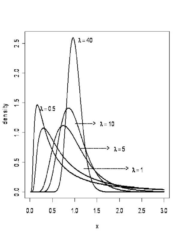
The probability density function (pdf) of IG distribution, IG( , )μ λ , is defined as

1/ 2 2 3 2 ( , , ) exp ( ) , 0, 0, 0, 2 2 f x x x x x λ λ μ λ μ μ λ π μ ⎧ ⎫ ⎛ ⎞ =_{⎜ ⎟ ⎨}− − _⎬ > > ⎝ ⎠ ⎩ ⎭ > (1.1)

where μ is the mean parameter and λ is the scale parameter. We present some density curves in Fig.1.1 and Fig. 1.2 for various values of μ at λ= and 1 λ at

1

Fig. 1.2 Density functions of IG( , )μ λ for fixed μ =1 and five values of λ

In Fig. 1.1 and Fig. 1.2, the density of IG distribution varies from the highly right-skewed to almost symmetric for different parameter configurations. Hence, the inverse Gaussian distribution is very flexible in describing various data.

The inference methods of the IG model are very analogous to those of the Gaussian model; for example, a very common problem in applied field is to compare the means of several Gaussian populations, i.e.

0 : 1 2 I

H μ = μ =_L=μ vs. H_A: not all ' are equalμ_i s . (1.2) If the variance of each population is homogeneous, the analysis of variance (ANOVA) can be used to perform the test. Similarly, the analysis of reciprocals (ANORE) can also be used to test the equality of means of several IG samples if all scale parameters among groups are assumed to be equal (Tweedie, 1956 ; Chhikara and Folks, 1989). The testing procedure will be briefly introduced in Remark 1. But when the scale parameters are non-homogeneous, the ANORE fails to solve the problem as ANOVA fails to test (1.2) when these populations are not homogeneous. Tian (2005) proposed a method to test the equality of IG means under heterogeneity based on generalized test variable method. However, if the null hypothesis is not been rejected, the inferences for the common mean remain unsolved. Therefore, in this paper, we would like to estimate and construct the 100(1−α)% confidence interval for the common mean of several non-homogeneous IG populations. Our method is based on a higher order asymptotic likelihood based method. This method, in theory, has a higher order accuracy, , and is very accurate even when the sample size is small. Reid (1996) gave some review and annotation of the development. The method has also been applied to solve many practical problems involving interval estimation for a skewed distribution, e.g. Wu et al. (2002) applied this procedure to make the confidence interval estimation of the ratio of two independent lognormal distribution, Wu et al. (2003) presented a confidence interval for a log-normal mean based on this

-3/2

(

method; Wu and Wong (2004) used the method to improve the interval estimation for the two-parameter Birnbaum-Saunders distribution; Tian and Wilding (2005) used the method to construct confidence interval for the ratio of means of two independent IG distributions, etc. In our case, the likelihood-based method gives a satisfactory result as well.

Remark 1. One of the resemblances between the IG distribution and the ordinary

Gaussian distribution is the method for the analysis of residuals. We are familiar with the analysis of variance (ANOVA) in normal inference theory, Tweedie (1956) introduce the so called analysis of reciprocals (ANORE) for the inverse Gaussian distribution. The procedure is as follows:

Assume that there are components in the th populations and each population is distributed as

i

n i

IG( , )μ λ_i , whereμ_i, i=1,..., and I λare unknown. Further assume the random samples Xij, 1,..., , 1,...,i= I j = ni

I

are independent. We are interested in the problem of testing (1.2)

The likelihood function, denoted by L(μ₁,...,μ λ_I, ;X_ij =x_ij, 1,..., , 1,...,i= I j= n )is proportion to 2 2 2 1 1 ( ) exp( ) 2 i N I n ij i i j i ij x x μ λ λ μ = = − −

∑∑

(1.3)

where . Differentiation with respect to

1 I i i N =

=

∑

n μ_i and λ yields the following

maximum likelihood estimates (MLEs), θˆ=(μˆ₁,...,μ λˆ_I, )ˆ , where

1 1 1 1 1 1 ˆ , ˆ _{( )} i i n i ij i j i n I ij i i j x x n N x μ λ = − − = = = = = −

∑

∑∑

1 . x− (1.4)

1 1 1 1 0 1 1 1 ˆ , ˆ _{( )} i i n I ij i j n I ij i j x x n N x μ λ = = − − = = = = = −

∑∑

∑∑

x . (1.5)

The likelihood ratio can be reduced to

2 1 1 0 ˆ ˆ o N N Q Q N λ λ − − Λ = ≡ (1.6)

Note that Qcan be decomposed into

₀ 1 1 1 I i i i Q Q n x− Nx− Q Q = = +

∑

− ≡ 0 + 1 (1.7)

It is easy to verify that λQ₀ follows a chi-squared distribution with degrees of freedom N−Iwhile λQ1 is a chi-squared distribution with degrees of freedom of

(I−1) and are independent. It follows that the likelihood ratio test statistic 1 and o Q Q 1 1, 0 ( ) ~ ( 1) I N I N I Q F I Q − − − − , (1.8)

where F_{I−1,N I−} is the F-distribution with degrees of freedom I−1 and and the

N−I

α level rejection region is given by solving the following inequality 1 1, ,1 0 ( ) ( 1) I N I N I Q F I Q − − −α − > − . (1.9)

For illustration examples of ANORE, see Chhikara and Folks (1989) and Seshadri (1999) for further details.

This article is organized as follows. In section 2, we will briefly introduce the properties of IG distribution and the concepts of the signed log-likelihood ratio statistic and a higher order asymptotic method. Then the method is applied to construct a confidence interval for the common mean of several independent IG populations in section 3. The classical procedure under the assumption of identical scale is also described in section 3. We will present two numerical examples and two

simulation studies in section 4 to illustrate the merits of our proposed method. Some concluding remarks are given in section 5.

2. A general review

In section 2.1 we give some basic characteristics of the IG distribution and some useful sampling distributions which will be used in later analysis. The main appeal of this article, the likelihood based inference technique, will be introduced in section 2.2.

2.1 Some properties of IG distribution

Let X be an inverse Gaussian distributed variate with parameters μ and λ. The probability density function of X is given in (1.1), and the distribution function can be written in terms of the distribution function of the standard normal variate, ( ) F x ( )x Φ , as F x( ) [ (x 1)] exp(2 ) [ (x 1)], x 0 x λ λ λ μ μ μ μ = Φ − + Φ − + > . (2.1)

The characteristic function of X is given by 1 2 2 2 ( ) exp[ (1 (1 ) )] X it C t λ μ μ λ = − − , (2.2) and the moment generating function can be obtained fromC_X( )t , i.e.,

1 0 ( 1 )! 2 ( ) ( ) . !( 1 )! t t X j t j M t j t j λ μ μ − t − = − − = − −

∑

(2.3) Differentiating the moment generating function with respect to for the first and second order at , we can obtain the mean and the variance of

t 0 t= X as ( ) E X =μ and 3 var( )X μ λ = , respectively.

For a random sample X X₁, ₂,...,X from IG_n ( , )μ λ , the uniformly minimum

variance unbiased estimators (UMVUEs) of μ and λ−1

are 1 1 n i i X X n = =

∑

and

W = 1 1 1 ( 1 n i i n = X − −

∑

1 )

X , respectively, and the minimum sufficient statistics of ( , )μ λ

are ( , )T T_{1 2} , where ₁ and

1 n i i T = =

∑

X 2 1 1 n i i T X =

=

∑

. It is worthy to notice that ~

X IG( ,μ λ and n ) (n−1)W ~ 1χ_n2₁

λ − , (2.4)

and that these two statistics are independently distributed. The proof can be found in Chhikara and Folks (1989).

Remark 2. Let X ~ IG( , )μ λ and Λ~ _λ1χn2 be two independent random variables,

then 1 2 2 2 ( ) ~ X X λ μ μ χ −

and its distribution is independent of λΛ~χ_n2 . Let

1/ 2 ( ( ) n X X ) μ μ Μ Λ −

= , then the distribution of Μ is the truncated Student’s variable with degrees of freedom and

t

n Μ has the distribution with 1 and degrees 2

of freedom. (Chhikara and Folks, 1989)

F n

From (2.4) and Remark 2, we know that

2 2 1 2 ( ) ~ n X X λ μ _χ μ − which is independent of 2 1 1 (n−1)W ~ λχn− . Let 1/ 2 ( ( ) n X U XW ) μ μ − = (2.5)

then the distribution of U is the truncated Student’s t with degrees of freedom and ~

1

n−

2

U F_1,n−1.

2.2 The likelihood-based inference

Let X (X₁,...,X_n)

% = be an independent sample from some distribution and

( ) ( ; )

l θ l θ X x

% %

= = be the log-likelihood function based on the sample data. Suppose θ is the p-dimensional vector parameters that can be partitioned into( , )μ λ with μ

being the parameter of interest with dimension 1, and λ being the nuisance parameters with dimensions p−1. The signed log-likelihood ratio r( )μ for inference

on μ is defined as (2.6) where 1/ 2 ˆ ˆ ˆ ( ) sgn( ){2[ ( ) ( )]} , r μ = μ μ− l θ −l θ_μ ˆ _{( , )ˆ} ˆ

θ = μ λ is the overall maximum likelihood estimator (MLE) of θ and ˆ _{( , )}ˆ

μ μ

θ = μ λ is the constrained MLE of θ for a given μ . Cox and Hinkley (1974) verified that r( )μ is asymptotically distributed as the standard normal distribution

with first-order accuracy O n( -1/2). A 100(1−α)% confidence interval for μ based on

( )

r μ can be obtained by

{ :| ( ) |μ r μ ≤z_{α/ 2}}, (2.7) where z_{α/ 2} is the 100(1−α/ 2)th percentile of the standard normal distribution. Since the signed log-likelihood ratio statistic is quite inaccurate when the sample size is small, Barndorff-Nielsen (1986, 1991) proposed a higher order likelihood-based method which is known as the modified signed log-likelihood ratio,

*( ) ( ) ( ) log{1 ( )}, ( ) q r r r r μ μ μ μ μ − = + (2.8) where r( )μ is the sign log-likelihood ratio statistic and q( )μ is a statistic which can

be expressed in various forms depending on the information available. For most of the conditions, q( )μ is not easy to obtain. Thomas (1999) presented an approximation to

( )

q μ with error of O n( −1) and hence r*( )μ . A widely applicable formula for q( )μ

that ensures the -3/2 accuracy provided by Fraser et al. (1999) is defined as ( O n ) 1/ 2 ; ; ; ; ˆ ˆ ˆ ˆ ( ) ( ) ( ) ( ) ( ) , ˆ ˆ ( ) ( ) V V V V l l l j q l j μ λ μ θθ θ λλ θ θ θ θ μ θ θμ ⎧ ⎫ − _{⎪ ⎪} = _{⎨ ⎬} ⎪ ⎪ ⎩ ⎭ (2.9)

where j_θθ( )θˆ is the p×p observed information matrix and j_λλ(θˆ_μ) is the observed nuisance information matrix and

; ; ' ' ' ; ; ; ˆ ˆ ˆ ( ) ( ) ( ) ˆ ˆ ˆ ( ) , ( ) V and ( ) V V V V l l l l l l V μ μ μ λ μ θ θ θ θ θ θ θ θ θ θ λ θ ∂ ∂ ∂ = = = ∂ ∂ ∂ .

The vector array V =( ,...,v₁′ vp′) in (2.9) where vi ={vi,1,...,vi n, }, , is

obtained from a vector pivotal quantity

1,..., i= p 1 1 ( ; ) ( ( ; ),..., _n( ; ))_n R xθ = R x θ R x θ % by 1 ˆ ( ; ) ( ; ) ( R x ) ( R x V x ) ,_θ θ θ θ − ∂ ∂ = − ∂ ∂ (2.10) where the distribution of R x_i( ; )_i θ is free of the parameters. The choice of the pivotal quantity will be briefly discussed in Remark 4. The quantity l_;V( )θ is the likelihood

gradient with ; ' 1 ( ) { ( ; ),..., ( ; )} V p d d l l x l dv dv θ θ θ % % = x , (2.11) where _{; ,} 1 1 ( ) ( , ) ( ) , 1,..., , 1,..., j n n x i j ij j j i j d l l x l v v i p j dv x θ θ θ = = ∂ = ⋅ = ⋅ = = ∂

∑

∑

n .

Note that achieves third-order accuracy to a standard normal distribution (Fraser et al. 1999). Therefore, a 100

*

r

(1−α)% confidence interval for μ based on r*( )μ is given by

. (2.12)

Remark 3. Notice that the procedure we mention above is performed for one population. If the inference problem involves

*

/ 2

{ :|μ r ( ) |μ ≤z_α }

I independent populations, some modifications are needed in applying this method. First, we put all the observations from the I distinct random samples together. Denote the set of observations by X

% ,

where . For each component in

1 2 11 1 21 2 1 ( ,..., , ,..., ,..., ,..., ) I n n I X = X X X X X X % In X % , we

construct a corresponding pivotal quantity, R Xij( ij, )θ , 1,..., i= I ,j=1,....ni, then

( )

q μ and r*( )μ can be constructed in similar manner as we mentioned above.

the computation of q( )μ (Fraser et al. 1999). A simple and easy choice is given by the

distribution function which is uniformly distributed. In fact, the choice of the pivotal quantity has crucial impact on the computation of the modified signed log-likelihood ratio algorithmatically. A choice which contains more information about the sample is preferred.

Remark 5. q( )μ in (2.9) can be expressed in various forms. It is different from the

quantity 1/ 2 ˆ ˆ ˆ ; ; ; ˆ ; ˆ ˆ ˆ ˆ ( ) ( ) ( ) ( ) ( ) , ˆ ˆ _{( )} ( ) l l l j q j l μ μ θθ θ θ λ θ λλ μ θ θ θ θ θ θ μ θ θ ⎧ ⎫ − _{⎪ ⎪} = _{⎨ ⎬} ⎪ ⎪ ⎩ ⎭ (2.13) where ˆ ˆ ; ; ˆ ˆ ˆ ; ; ; ˆ _{ˆ ˆ} ( ) ( ) ( ) ˆ ˆ ˆ ( ) , ( ) , ( ) ˆ l l l l l l μ θ θ μ θ λ θ θ θ θ θ _{θ θ θ} θ θ θ θ θ θ λ θ θ = _{= =θ} ∂ ∂ ∂ = = = ∂ ∂ ∂

given by Barndorff-Nielsen (1991) and Barndorff-Nielsen & Cox (1994) for computing r*( )μ . Both variants of r*( )μ can reach third-order accuracy, although

*

( )

r μ can be obtained through different forms. The expression in (2.13) involves differentiation with respect to ˆθ, if there is no analytic form of MLEs, then sometimes such q( )μ is difficult or impossible to obtain. For example, as for our

problem, the inference for the common mean of I independent IG populations, there are I+1 parameters and 2I minimal sufficient statistics which is the so-called

curved exponential model,

(2 ,I I+1) q( )μ in (2.13) is not easy to apply since the

MLEs do not have closed form, so the computation of the derivative with respect to ˆ

θ is not available. On the other hand, q( )μ in (2.9) is easy to implement

algorithmically. Such a q( )μ is quite flexible; hence we will use it to perform the

3. Inferences for the common mean of several independent IG

populations

In this section we apply the procedure we present in section 2 to construct the confidence interval. The derivation for the general case will be presented in section 3.1. The two independent IG populations case will be discussed in section 3.2. At last, we derive the t-like confidence interval under the assumption of homogeneity for comparison purpose. All the results will be utilized in the simulation in the next section.

3.1 The likelihood-based confidence interval in the general case

Suppose ( ₁,..., ), 1, 2,.., ,

i

i i in

X = X X i= I are I independent populations from IG ( ,μ λ_i). The parameters,θ =( ,μ λ₁,...,λ_I), contain μ being the parameter of interest and ( ,...,λ₁ λ_I)being the nuisance parameters. The log-likelihood function is

1 1 2 1 1 1 1 1 1 1 1 ( ; ,..., ) 1 3 1 1 1 log log . (3.1) 2 2 2 2 2 i i i I I n n n I I I I I i i i ij i ij i i i i j i j i i j ij l X x X x n x x n x θ λ _{λ λ} λ π μ μ = = = = = = = = = = =

∑

−

∑∑

−

∑∑

+

∑

−

∑∑

Differentiating the log-likelihood function (3.1) with respect to θ for the first order yields the following results:

2 3 2 1 1 1 2 2 2 1 1 ( ) 1 1 ( ) 1 1 1 , 1,..., . 2 2 2 i i i n I I i i i i i j ij n n i i ij j j i i ij l n x n n l x i I x λ θ _λ μ μ μ θ λ λ μ μ = = = = = ∂ − = + ∂ ∂ _{= + − − =} ∂

∑

∑∑

∑

∑

(3.2)

The overall MLEs θˆ=( ,μ λˆ ˆ₁,...,λˆ_I) can be uniquely obtained by solving the non-linear system (3.2) simultaneously. It seems that in our problem, there is no analytic form for the overall MLEs. Therefore, some numerical facility is needed to

get the numerical solutions. Furthermore, the constrained MLEs for a given ,1 , ˆ _{( ,} ˆ _,..., ˆ ₎ I μ μ θ = μ λ λ_μ μ are 2 , 2 1 1 1 ˆ _{, 1,...,} 1 (2 ) i i i i n n i i i i n i n x x μ μ λ μ μ = = − = −

∑

−

∑

I = . (3.3)

Choosing a vector of pivotal quantity { ₁₁,..., }

I In R= R R with 2 2 ( ) , i ij ij ij x R x λ μ μ − = , then 1,.., ; 1,.., _i

i= I j = n R_ij ~χ₁2 with the distribution free of any unknown parameters. Differentiating R_ij with respect to xand θ , we have

2 2 1 2 2 ( ) , if ; else 0 ( ) ij ij ij k i ij k R x R j k x x x μ λ μ − ∂ ∂ = = = ∂ − ∂ ; 3 2 ( ) ij i ij R λ x μ μ μ ∂ − − = ∂ ; 2 2 ( ) if ; else 0 ij ij ij k ij k R x R j k x μ λ μ λ ∂ − ∂ = = ∂ ∂ = . (3.4) Thus 1 1 2 2 2 2 2 2 2 2 1 1 11 1 2 2 2 2 2 2 2 2 1 11 1 1 1 ( ) [ ,..., ,..., ,..., ] ( ) ( ) ( ) ( I I n _I I n I I I In x x x x R diag x x x x x μ μ μ μ ) n λ μ λ μ λ μ λ μ − ∂ = ∂ − − − − , (3.5)

where diag[.] is the abbreviation of the diagonal matrix.

Furthermore, ' ' ' ₁' ' 1 ( ) [( ) , ( ) ,..., ( ) ] [ ,..., _I ] I R R R R h h θ μ λ λ +1 ∂ ₌ ∂ ∂ ∂ ₌ ∂ ∂ ∂ ∂ with 1 11 1 11 1 1 3 3 3 2 ( ) 2 ( ) 2 ( ) 2 ( ) ( x ,..., xn ,..., I xI ,..., I x I ) h λ μ λ μ λ μ λ In₃ μ μ μ μ − − − − − − − − = μ _{ 1 1 2 2 1 1 2 2 1 ( ) ( ) (0,..., 0 , ,..., j , 0...., 0) , 1,..., j _j k k jn j j j jn n x x h j x x μ μ μ μ − = + − − = = ∑ I. (3.6)

' ' 1 1 1 ˆ ( ,..., _I ) ( R) ( ) V v v R x θ _θ − + ∂ ∂ = = − ∂ ∂ 1 1 1 1 1 2 2 2 2 11 11 11 11 1 11 2 1 1 1 1 1 1 21 21 2 21 2 2 1,1 1,1 2 2 1 1,1 ˆ 2 ( ) 0 0 ˆ ˆ( ˆ) ( ˆ) ˆ 2 ( ) 0 0 ˆ ˆ( ˆ) ( ˆ) ˆ ( ) 0 ˆ _{( ˆ)} 0 0 ˆ ( ) ( ˆ) 0 0 ˆ _{( ˆ)} ˆ _{( ˆ)} 0 0 n n n n n n n I I n I I x x x x x x x x x x x x x x x x x x x μ μ μ λ μ μ μ μ λ μ μ λ μ μ μ λ μ λ μ L M M M M M M L M O M M M M O M M M O M − − − − − − + + − − + + − − + − − − − + + = 0 0 M M 1 1 1 1, 1, 1 1, 2 1 1 1 1 1 2 ˆ ( ) ˆ _{( ˆ)} 0 0 0 0 ˆ 2 ( 0 0 ˆ ˆ( ˆ) ( ˆ) ˆ 2 ( 0 0 0 ˆ ˆ( ˆ) ( ˆ) I I I I I I I I I n I n I I n I I I I I I In In In In I In x x x x x x x x x x x μ λ μ μ μ μ λ μ ) ) x x μ μ μ λ μ M M M O M M M L M M M M M M M L − − − − − − − ⎡ ⎤ ⎢ ⎥ ⎢ ⎥ ⎢ ⎥ ⎢ ⎥ ⎢ ⎥ ⎢ ⎥ ⎢ ⎥ ⎢ ⎥ ⎢ ⎥ ⎢ ⎥ ⎢ ⎥ ⎢ ⎥ ⎢ ⎥ ⎢ ⎥ ⎢ ⎥ ⎢ ⎥ ⎢ ⎥ ⎢ ₋ ⎢ ₋ ⎢ + ⎢ ⎢ ⎢ ₋ ⎢ ₋ ⎢ + + ⎢ ⎢ ⎢ ₋ ⎢ ₋ ⎢ + + ⎣ ⎦ . ⎥ ⎥ ⎥ ⎥ ⎥ ⎥ ⎥ ⎥ ⎥ ⎥ ⎥ ⎥ ⎥

It remains to obtain the likelihood gradients, l_;V( ),θ lλ;V( )θ , lθ;V( )θ , and the fisher

information matrices j_θθ( )θ and j_λλ( )θ . Notice again that

' ; 1 1 ; ; ; ' ; 1 ; ; ; ; ' ; 1 ( ) ( ) ( ) ( ) [ ,..., ], ( ) ( ) ( ) ( ) [ ,..., ], ( ) ( ) ( ) ( ) ˆ ( ) [ , ,..., ], V I V V V V I V V V V V I l l l l V v v l l l l l l l l l λ θ θ θ θ θ θ θ θ θ λ λ λ θ θ θ θ θ θ μ λ λ + ∂ ∂ ∂ = = ∂ ∂ ∂ ∂ ∂ ∂ = = ∂ ∂ ∂ ∂ ∂ ∂ ∂ = = ∂ ∂ ∂ ∂ where 1 ; , ( 1) 1 1 ( ) , 1,... ( , , ) i ij i n I x k j i n i j k l v k l v θ _θ − + − × = = = ∂ ₌ ∂

∑∑

p 1 1 ; 1, ( 1) ; 1, ( 1) 1 ; 1 1 1 ( ) ,..., ( ) [ ( i i ij i ij i n n I I x j i n x I j i n i j i V j l l_μ v l_μ v θ θ θ μ + − × − + + − × − = = = = ∂ = ∂

∑∑

∑∑

) ], 1 1 ; 1, ( 1) ; 1, ( 1) 1 1 1 1 ; ( ) ,..., ( ) ], 1 ( ) [ ,..., i i m ij i m ij i n n I I x j i n x I V i i j i j m j n l v l v m l I λ θ λ θ θ λ + − × − + + − × − = = = = = ∂ = ∂

∑∑

∑∑

.

Therefore the complete results are 1 1 ; 1, ( 1) 1 1 ; ; 1, ( 1) 1 1 ( ) ( ) , ( ) i ij i i ij i n I x j i n i j V n I x I j i n i j l v l l v θ θ θ − − + − × = = + + − × = = ⎡ ⎤ ⎢ ⎥ ⎢ ⎥ ⎢ ⎥ = ⎢ ⎥ ⎢ ⎥ ⎢ ⎥ ⎣ ⎦

∑∑

∑∑

M 1 1 1 1 ; 1, ( 1) 1 1 1 − ; 1, ( 1) 1 1 1 1 ; ; 1, ( 1) ; 1, ( 1) 1 1 1 1 ( ) ( ) ( ) , ( ) ( ) i i ij i I ij i i i ij i I ij i n n I I x j i n x I j i n i j i j V n n I I x I j i n x I j i n i j i j l v l v l l v l v λ λ λ λ λ θ θ θ θ θ − − − − + − × + + − × = = = = + + − × + + − × = = = = ⎡ ⎤ ⎢ ⎥ ⎢ ⎥ ⎢ ⎥ = ⎢ ⎥ ⎢ ⎥ ⎢ ⎥ ⎣ ⎦

∑∑

∑∑

∑∑

∑∑

L M M L 1 1 1 1 1 1 1 ; 1, ( 1) ; 1, ( 1) ; 1, ( 1) 1 1 1 1 1 1 ; ; 1, ( 1) ; 1, ( 1) ; 1 1 1 1 ( ) ( ) ( ) ( ) ( ) ( ) i i i ij i ij i I ij i i i ij i ij i n n n I I I x j i n x j i n x j i n i j i j i j V n n I I x I j i n x I j i n i j i j l v l v l v l l v l v l μ λ λ θ μ λ λ θ θ θ θ θ θ − − − − + − × + − × + − × = = = = = = + + − × + + − × = = = = =

∑∑

∑∑

∑∑

∑∑

∑∑

L M M M M L 1, ( 1) ₁ 1 1 . ( ) i ij i n I x I j i n i j v θ _{+ + − × −} = = ⎡ ⎤ ⎢ ⎥ ⎢ ⎥ ⎢ ⎥ ⎢ ⎥ ⎢ ⎥ ⎢ ⎥ ⎣

∑∑

⎦

The observed information matrix and the observed nuisance information matrix can be calculated by multiplying the Hessian matrix for the log-likelihood function by (-1) . The results are given below.

1 2 1 2 1 2 1 2 4 3 2 2 2 3 2 1 1 1 1 1 1 1 1 1 2 3 2 1 1 2 2 2 2 3 2 1 2 2 3 2 1 3 2 0 0 0 2 ( ) 0 0 2 0 0 0 0 0 0 0 2 i I I n n n n I I i ij i i i i I Ii i j i i i i n i i n i i n Ii I I i I x n n x n x n x n n x n n j x n n θθ λ λ 3 x μ μ μ μ μ μ μ μ μ μ λ θ μ μ λ μ μ λ = = = = = = = = = ⎡ ⎤ − − − − ⎢ ⎥ ⎢ ⎥ ⎢ ⎥ − ⎢ ⎢ ⎢ ⎢ = − ⎢ ⎢ ⎢ ⎢ ⎢ ⎢ ₋ ⎢⎣ ⎦

∑∑

∑

∑

∑

∑

∑

∑

∑

L L L M M M M O M M M O L ⎥ ⎥ ⎥ ⎥ ⎥ ⎥ ⎥ ⎥ ⎥ ⎥ ⎥ M and

1 2 1 2 0 2 ( ) 0 2 I I n j n λλ λ θ λ ⎡ ⎤ ⎢ ⎥ ⎢ ⎥ = ⎢ ⎥ ⎢ ⎥ ⎢ ⎥ ⎢ ⎥ ⎣ ⎦ O .

Apply the above quantities to (2.8) and (2.9),

1/ 2 ; ; ; ; ˆ ˆ ˆ ˆ ( ) ( ) ( ) ( ) ( ) ˆ ˆ ( ) ( ) V V V V l l l j q l j μ λ μ θθ θ λλ θ θ θ θ μ θ θ_μ ⎧ ⎫ − _{⎪ ⎪} = ⎨ ⎬ ⎪ ⎪ ⎩ ⎭

and then *( ) ( ) ( ) log{1 ( )} ( ) q r r r r μ μ μ μ μ − = + can be obtained.

Although the values of r and can be obtained here, in general, some simple numerical iteration procedure is needed to solve the upper bound limit and lower bound limit. In this thesis we use the so-called secant method (or the modified Newton-Raphson method) to obtain the confidence limit; the algorithm is summarized as follows:

*

r

Step 1: Give the tolerance ε for the purpose of accuracy; Step 2: Select δ for the purpose of numerical differentiation; Step 3: Give the initial estimate μ₀ to start the iteration; Step 4: Compute / 2 0 1 0 0 0 [ ( )] [ ( ) ( )] / 2 Z r r r α μ μ μ μ δ μ δ δ − = + + − − (3.7)

Step 5: If μ μ₁− ₀ > , replace ε μ₀ with μ₁ and return to Step 4 again,

otherwise take the latest μ₁ as the lower bound limit of the 100(1−α)% confidence interval.

Replacing Z_{α/ 2} with Z_{1−α/ 2} in (3.7), we can obtain the upper bound limit for the

100(1−α)% confidence interval of the common meanμ . Similarly, the confidence interval based on r*can be obtained by substituting r* for in (3.7). r

3.2 The likelihood-based confidence interval when I=2

For the purpose of illustration, we present the derivation of the confidence interval for the common mean of two independent IG populations. Let

1 1 11,..., 1n ~ IG( , )1 X =X X μ λ % and 2 2 21,..., 2n ~ IG( , 2) X = X X μ λ

% be two independent inverse Gaussian samples. The

log-likelihood function based on the observations is

1 1 1 2 2 2 1 1 1 1 1 1 2 2 1 1 2 2 1 2 1 1 1 1 1 2 2 2 2 2 2 2 1 1 1 2 3 1

( ; , ) log log log

2 2 2 2 2 2 2 3 1 log . (3.8) 2 2 2 n n n i i i i i i n n n i i i i i i n n l X x X x x x x n x x x n λ λ λ λ θ λ π μ μ λ λ λ μ μ = = = = = = = = = − − + − + − − + −

∑

∑

∑

∑

∑

∑

% % % % π ˆ

The MLEs and the constrained MLEs are θˆ=( ,μ λ λˆ ˆ₁, ₂) and θˆ_μ =( ,μ λ λˆ_1μ, ˆ_2μ) , respectively . Take 2 2 ( ) i ij ij ij x R x λ μ μ −

= to be the pivotal quantity as we mentioned earlier and

differentiate R_ij with respect to x and θ, we then have

1 1 2 2 2 2 11 2 2 1 11 2 2 1 2 2 1 1 1 2 2 21 2 2 2 21 2 2 2 2 2 2 2 ( ) ( ) ( ) ( ) ( )

0

0

n n n n x x x x R x x x x x μ λ μ μ λ μ μ λ μ μ λ μ O O − ⎡ ⎤ ⎢ ₋ ⎥ ⎢ ⎥ ⎢ ⎥ ⎢ ⎥ ⎢ ⎥ ⎢ ₋ ⎥ ∂ _{⎢ ⎥} = ⎢ ⎥ ∂ ⎢ ⎥ − ⎢ ⎥ ⎢ ⎥ ⎢ ⎥ ⎢ ⎥ ⎢ ⎥ − ⎢ ⎥ ⎣ ⎦ and

1 1 1 2 2 2 2 1 11 11 3 2 11 2 1 1 1 3 2 1 2 2 21 21 3 2 21 2 2 2 2 3 2 2 2 ( ) ( ) 0 2 ( ) ( ) 0 ( ) 2 ( ) ( ) 0 2 ( ) ( ) 0 n n n n n n x x x x x x z x x x x x x λ μ μ μ μ λ μ μ μ μ θ λ μ μ μ μ λ μ μ μ μ M M M M M M ⎡ − − − ⎤ ⎢ ⎥ ⎢ ⎥ ⎢ ⎥ ⎢ ⎥ − − − ⎢ ⎥ ⎢ ⎥ ∂ _{⎢ ⎥} = ⎢ ⎥ ∂ − − − ⎢ ⎥ ⎢ ⎥ ⎢ ⎥ ⎢ ⎥ ⎢− − − ⎥ ⎢ ⎥ ⎢ ⎥ ⎣ ⎦ . So ₁' '_{2 3}' 1 ˆ ( , , ) ( ) ( ) V v v v R x R θ θ − ∂ ∂ = = − ∂ ∂ 1 1 1 1 1 2 2 2 2 2 11 11 11 11 1 11 2 1 1 1 1 1 1 2 21 21 21 21 2 21 2 2 2 2 2 2 ˆ 2 ( ) 0 ˆ ˆ( ˆ) ( ˆ) ˆ 2 ( ) 0 ˆ ˆ( ˆ) ( ˆ) ˆ 2 ( 0 ˆ ˆ( ˆ) ( ˆ) ˆ 2 ( 0 ˆ ˆ( ˆ) ( ˆ) n n n n n n n n n x x x x x x x x x x x x x x x x x x μ μ μ λ μ μ μ μ λ μ μ μ μ λ μ 2 2 ) ) n x x μ μ μ λ μ M M M M M M ⎡ − ⎤ − ⎢ _{+ +} ⎥ ⎢ ⎥ ⎢ ⎥ ⎢ ⎥ − ⎢ ⎥ − ⎢ _{+ +} ⎥ ⎢ ⎥ = ⎢ ₋ ⎥ ⎢ ₋ ⎢ + + ⎢ ⎢ ⎢ ₋ ⎢ ₋ ⎢ + + ⎣ ⎦ ⎥ ⎥ ⎥ ⎥ ⎥ ⎥ ⎥ .

Moreover, the likelihood gradients are

1 2 1 2 2 1 1 1 2 2 2 2 2 2 2 1 1 1 1 1 2 2 1 1 1 1 ; 2 2 1 1 1 1 1 2 2 2 2 2 2 2 2 2 2 ˆ ˆ ˆ ˆ 2 3 2 3 ( ) ( ˆ( ˆ) 2 2ˆ 2 ˆ( ˆ) 2 2ˆ 2 ˆ ˆ ˆ ( ) 3 ( ) ( ) ˆ_{( ˆ) 2 2ˆ 2} ˆ ˆ ˆ ( ) 3 ( ) ˆ _{( ˆ) 2 2ˆ 2} n n i i i i i i i i i n i i V i i i i i i i i i x x x x x x x x x x l x x x x x x x x λ λ λ λ μ μ μ μ μ μ μ λ λ θ μ λ μ μ λ λ μ λ μ = = = ⋅ − − + ⋅ − − + + − = ⋅ − − + − _{⋅ − −} +

∑

∑

∑

2 1 , n i= ⎡ ⎤ ⎢ ⎥ ⎢ ⎥ ⎢ ⎥ ⎢ ⎥ ⎢ ⎥ ⎢ ⎥ ⎢ ⎥ ⎢ ⎥ ⎣

∑

⎦ 2 ) i

1 2 1 2 2 2 1 2 2 2 2 2 1 1 1 1 2 2 1 1 ; 2 2 1 1 1 1 2 2 2 2 1 2 2 2 2 1 1 2 1 1 ( ) ( ˆ( ˆ) 2 2ˆ ˆ( ˆ) 2 2ˆ ˆ ( ) 1 1 ( ) ( ) 0 ˆ_{( ˆ) 2 2ˆ} ˆ ( ) 1 1 0 ( ˆ _{( ˆ) 2 2ˆ} n n i i i i i i i i n i i V i i i n i i i i i x x x x x x x x l x x x x x x λ μ μ μ μ μ μ μ θ μ λ μ μ μ λ μ = = = = ⎡ ⎤ ⋅ − ⋅ − ⎢ ⎥ + + ⎢ ⎥ ⎢ ₋ ⎥ ⎢ ⎥ = ⋅ − ⎢ + ⎥ ⎢ ⎥ − ⎢ _{⋅ −} ⎥ ⎢ ₊ ⎥ ⎣ ⎦

∑

∑

∑

∑

) ) and 1 2 1 1 2 2 2 2 1 2 4 2 2 1 1 1 1 1 1 2 2 1 1 1 1 ; 3 2 2 1 1 1 1 1 1 2 2 3 ˆ _{2 2 1 1 2 1 1} ( ) ( ˆ ˆ ˆ( ˆ) 2 2ˆ ˆ( ˆ) 2 2ˆ ˆ ˆ ( ) ( ) 1 1 1 ( ) ( ) 0 ˆ ˆ ( ˆ) ( ˆ) 2 2ˆ ˆ ( ) 1 ˆ ( i n n n ij i i i i j ij i i i i i i n n i i i i V i i i i i i i x x x x x x x x x x x x l x x x x x θ λ μ μ μ μ μ μ μ μ μ μ θ μ μ λ μ μ μ μ = = = = = = ⋅ ⋅ − ⋅ + + + − − = − ⋅ − + + − −

∑∑

∑

∑

∑

∑

2 − 2) 2 2 2 2 2 2 1 2 1 2 2 2 . ˆ ( ) 1 1 0 ( ˆ ˆ) ( ˆ) 2 ˆ n n i i i i i i i x x x x x μ μ λ μ μ = = ⎡ ⎤ ⎢ ⎥ ⎢ ⎥ ⎢ ⎥ ⎢ ⎥ ⎢ ⎥ ⎢ ⎥ − ⎢ _{⋅ −} ⎥ ⎢ _{+ +} ⎥ ⎣

∑

∑

2 )⎦

The observed Fisher information matrix and the observed nuisance information matrix are 1 1 1 1 2 2 2 2 1 1 2 2 4 3 4 3 2 3 2 1 1 1 2 3 2 1 2 2 2 2 3 2 2 3 2 3 2 ( ) 0 2 0 2 s n s n n s n s n s n j n s n θθ λ λ λ λ 3 μ μ μ μ μ μ μ μ θ μ μ λ μ μ λ ⎡ ⎤ − + − − − ⎢ ⎥ ⎢ ⎥ ⎢ ⎥ =_⎢ − _⎥ ⎢ ⎥ ⎢ ⎥ − ⎢ ⎥ ⎣ ⎦ and 1 2 1 2 2 2 0 2 ( ) 0 2 n j n λλ λ θ λ ⎡ ⎤ ⎢ ⎥ ⎢ ⎥ = ⎢ ⎥ ⎢ ⎥ ⎣ ⎦ ,

where and . Finally, a 100

1 1 1 n i i s X = =

∑

_{1 2} 2 ₂ 1 n i i s X = =

∑

(1−α)% confidence interval of μ based on * ( )

r μ is then obtained by applying these quantities to (2.8) and (2.12).

3.3 Simple t-test confidence interval

inspired from the analysis of reciprocals (ANORE). This method can provide an exact confidence interval when the scale parameters are homogeneous. Suppose ( ₁,..., ), 1, 2,.., ,

i

i i in

X = X X i= I are I independent populations with

parameters ( ,μ λ_i) for each population, from (2.4) we know that

1 1 1 ~ ( , ) i n I ij i j X X IG N = = μ λN =

∑∑

and (N I W) ~ 1 χ_{N I}2 λ −

− are independent distributed,

where , 1 I i i N n = =

∑

1 1 ni i i j i j X X n = =

∑

and 1 1 1 1 ( i n I ij i i j W X N I − − = = = −

∑∑

1 ) X − . Moreover,

from Remark 2, we know ( _{1/ 2}

( ) N X XW ) μ μ −

is the truncated student’s distribution with degrees of freedom. Therefore, a two-sided

t

N−I 100(1−α)% for μ can be obtained by solving the following inequality

1/ 2 _{1 ,} 2 ( ) : ( ) N I N X t XW α μ μ μ − − ⎧ ₋ ⎫ ⎪ _< ⎪ ⎨ ⎬ ⎪ ⎪ ⎩ ⎭ 1/ 2 _{1 ,} 2 ( 1) : ( ) N I X N t XW α μ μ − − ⎧ ⎫ − ⎪ ⎪ ⎪ ⎪ =_⎨ < _⎬ ⎪ ⎪ ⎪ ⎪ ⎩ ⎭ .

The confidence interval is summarized as

1 1 1 1 1 2 2 2 1 1 2 1 , 1 , if 1 . , otherwise 1 , XW XW XW X t X t t N N XW X t N α α α α − − − − − − − ⎛ ⎞ ⎛ ⎞ + − − ⎜ ⎟ ⎜ ⎟ ⎜ ⎟ ⎜ ⎟ ⎝ ⎠ ⎝ ⎠ ⎛ ⎞ + ⎜ ⎟ ⎜ ⎟ ⎝ ⎧ ⎡ ⎤ ⎪ ⎢ ⎥ ⎪ ⎢ ⎥ ⎪ ⎣ ⎦ ⎨ ⎡ ⎪ _⎤ ⎢ _∞ ⎪ _⎥ ⎢ ⎪ _⎣ ⎦ ⎩ ⎠ 0 N > (3.9)

4 . Simulation studies and numerical examples

In this section, we first present a simulation to show the normal approximation of and . In section 4.2, we conduct a simulation study of the proposed procedure for different parameter configurations. In section 4.3, a real-life data and a simulated data are given as illustrations.

r r*

4.1 Normal approximation for r and r*

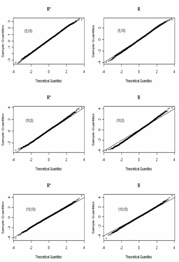
To show that the normal approximations for and are adequate, we conduct a simulation to show the validity and also to compare the extent of asymptotic of and

. We present the Q-Q plots for both and under the same parameter settings. For two populations, the sample sizes

r r* r * r r* r 1 2 ( ,n n )=(5,10) , (10, 5) and (10,10) and 1 2

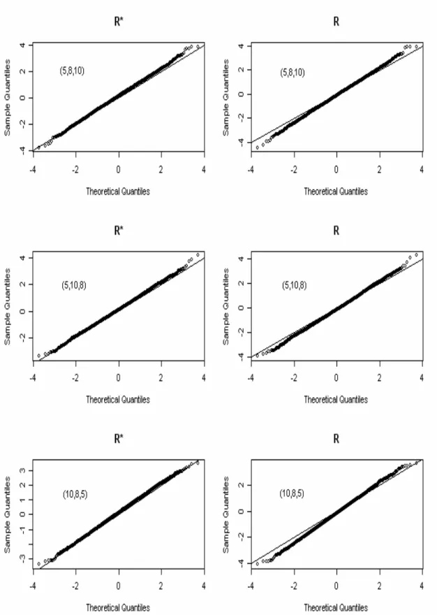
( ,μ λ λ, )= (1,0.2,1) are demonstrated. And the sample sizes (5,8,10),

(5,10,8) and (10,8,5) and

1 2 3

( ,n n n, )=

1 2 3

( ,μ λ λ λ, , )=(1, 0.1, 0.5,1) are chosen for three populations.

All the simulations are based on 5,000 repetitions. For two populations, the Q-Q plots are given in Fig. 4.1 and for three populations, the Q-Q plots are given in Fig. 4.2. Both Fig. 4.1 and Fig. 4.2 show that the asymptotic of is better than which is consistent as we expect. In these figures, we can see, most of the tail of the Q-Q plots of deviate off the straight line which is the indicator of normality whereas those of seem to overlap the straight line for most of the part. In short, is more accurate in approximating to the standard normal.

* r r r * r * r

Fig. 4.1 Q-Q plots for two populations at ( ,μ λ λ₁, ₂)=(1, 0.2, 1)

4.2 Simulation studies

To evaluate the accuracy of the proposed method, we present simulation studies of the confidence interval and type I errors applied to a variety of scale parameter configurations and different settings of sample size for two and three populations. We exhibit the coverage probabilities, the average lengths of the 95% confidence intervals and calculate type I errors based on , and simple t-test method. The results given in tables 1-4 below are based on 10,000 simulation runs for each combination. From the table 1 and table 2, we see that although the confidence intervals based on the directed log-likelihood ratio method, , have shortest average lengths comparing to the other two methods, the coverage probabilities are too short to attain the proposed coverage probabilities in each combination. The confidence intervals based on the simple t-test method also show a good performance on coverage probabilities, but these coverage probabilities decrease when the heterogeneity increases. Moreover, when the scale parameter is small related to

r r*

r

μ , then the intervals constructed by the simple t-test are unbounded (i.e., a one-sided interval). In these cases, the method gives less information about the target value than those based on and r. On the other hand, the confidence intervals based on higher order likelihood-based method, , not only have almost exact coverage probabilities in each combination (except for few pairs having large sample sizes with relatively small scale parameters), but the average lengths are also quite acceptable. Therefore, for the overall comparisons, the higher order likelihood-based method outperforms the other two methods.

*

r

*

Table 1

Simulation results of 95% confidence interval of μ=1 for two populations

*

r r simple t-test

1 2

( ,n n ) λ₁ λ₂

CP Length CP Length CP Length

(5,10) 0.2 1 0.951 9.387 0.923 1.637 0.954 ∞ 0.5 1 0.948 14.340 0.917 1.554 0.945 ∞ 1 3 0.952 1.054 0.926 0.786 0.943 1.024 3 10 0.947 0.456 0.920 0.387 0.939 0.486 1 10 0.948 0.477 0.923 0.409 0.933 0.791 (10,5) 0.2 1 0.931 23.093 0.847 1.368 0.955 ∞ 0.5 1 0.944 13.672 0.897 1.534 0.949 ∞ 1 3 0.949 1.958 0.906 0.967 0.950 1.506 3 10 0.948 0.598 0.903 0.464 0.949 0.623 1 10 0.947 0.840 0.925 0.573 0.951 1.361 (10,10) 0.2 1 0.951 7.914 0.929 1.659 0.958 ∞ 0.5 1 0.955 2.320 0.933 1.363 0.948 ∞ 1 3 0.945 0.873 0.924 0.708 0.946 0.918 3 10 0.945 0.410 0.921 0.360 0.947 0.456 1 10 0.949 0.459 0.926 0.399 0.947 0.795

Table 2

Simulation results of 95% confidence interval of μ=1 for three populations

*

r r simple t-test

1 2 3

( ,n n n , ) λ₁ λ₂ λ₃

CP Length CP Length CP Length

(5,8,10) 0.1 0.1 1 0.949 4.865 0.923 1.611 0.965 ∞ 0.1 0.5 1 0.949 3.382 0.922 1.456 0.959 ∞ 1 1 5 0.948 0.671 0.923 0.542 0.948 0.807 1 1 10 0.949 0.467 0.925 0.396 0.943 0.766 1 5 10 0.948 0.393 0.921 0.337 0.938 0.511 (5,10,8) 0.1 0.1 1 0.952 5.964 0.917 1.589 0.963 ∞ 0.1 0.5 1 0.948 3.784 0.918 1.492 0.952 ∞ 1 1 5 0.945 0.754 0.919 0.586 0.951 0.873 1 1 10 0.950 0.537 0.919 0.435 0.947 0.844 1 5 10 0.945 0.413 0.917 0.350 0.938 0.524 (10,8,5) 0.1 0.1 1 0.928 7.016 0.839 1.306 0.967 ∞ 0.1 0.5 1 0.946 5.952 0.889 1.467 0.965 ∞ 1 1 5 0.943 0.957 0.901 0.668 0.950 0.974 1 1 10 0.945 0.720 0.898 0.518 0.953 0.956 1 5 10 0.946 0.521 0.902 0.406 0.948 0.711

CP : Coverage probability; Length : Average length

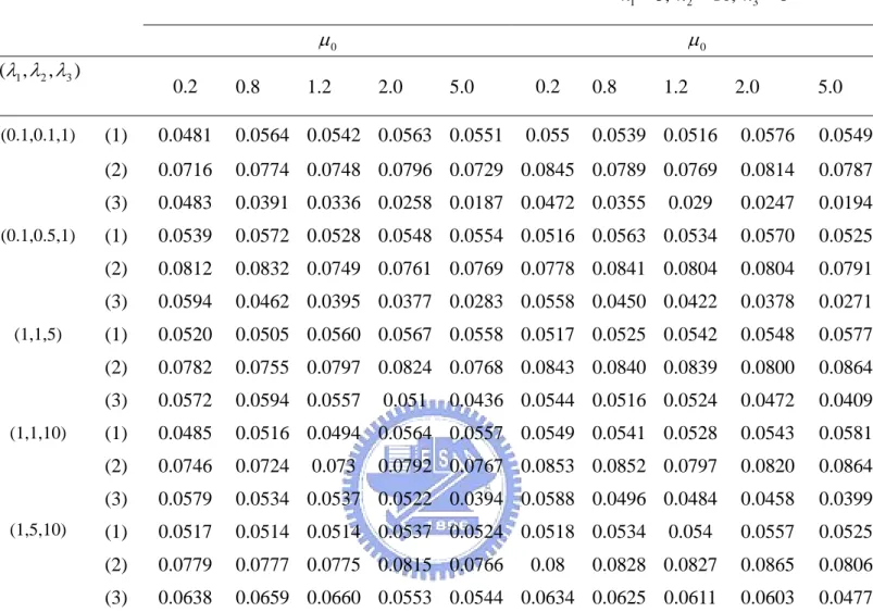
Furthermore, from tables 3 and 4, we can see the type I errors based on and are quite stable under different parameter configurations since the type I errors based on the simple t-test method decrease as the mean parameter under the null hypothesis increases. From tables 3 and 4, the type I errors based on are significantly better than that of since the type I errors based on are around 0.07 to 0.10 which are

*

r r

*

r

too large comparing to the nominal level 0.05. On the contrary, the type I errors based on are not only stable, but the values also close to the nominal level 0.05. Thus, we can say that the proposed procedure can deal with heterogeneity among populations and give robust and reliable results under different scenarios.

*

r

Table3: Type I errors for H₀:μ μ= ₀ vs. H₀:μ μ≠ ₀ at I=2 and α =0.05

1 5, 102 n = n = n₁ =10, 5n₂ = 0 μ μ₀ 1 2 ( ,λ λ ) 0.2 0.8 1.2 2.0 5.0 0.2 0.8 1.2 2.0 5.0 (0.2, 1) (1) 0.0522 0.0528 0.0529 0.0493 0.0506 0.055 0.0495 0.0567 0.0551 0.0524 (2) 0.0774 0.0746 0.075 0.0686 0.0702 0.1027 0.0903 0.0989 0.0912 0.0912 (3) 0.0615 0.0430 0.0489 0.0426 0.0324 0.0502 0.0378 0.0410 0.0381 0.0313 (0.5,1) (1) 0.0485 0.0562 0.0569 0.0533 0.0575 0.0528 0.056 0.0522 0.0552 0.053 (2) 0.0832 0.0862 0.0844 0.0813 0.0808 0.0901 0.095 0.0922 0.0922 0.0883 (3) 0.0555 0.0507 0.0514 0.0504 0.0509 0.0469 0.0515 0.0461 0.0434 0.0484 (1, 3) (1) 0.0526 0.0528 0.0500 0.0578 0.0564 0.0542 0.0548 0.0573 0.0570 0.0553 (2) 0.0783 0.0783 0.0744 0.081 0.079 0.0966 0.0985 0.0941 0.0939 0.0939 (3) 0.0583 0.0545 0.0503 0.0539 0.0524 0.0514 0.0471 0.0464 0.0535 0.0424 (1, 5) (1) 0.0507 0.0566 0.0517 0.0551 0.057 0.0585 0.0537 0.0558 0.0563 0.0575 (2) 0.0788 0.0803 0.0768 0.0779 0.079 0.1009 0.0936 0.099 0.098 0.0989 (3) 0.0634 0.0616 0.061 0.0573 0.0499 0.0502 0.0471 0.0465 0.046 0.0371 (1, 10) (1) 0.0528 0.055 0.0484 0.0559 0.0487 0.0559 0.0538 0.0517 0.0582 0.0571 (2) 0.0751 0.0759 0.0727 0.0777 0.0697 0.104 0.0977 0.0967 0.0997 0.0981 (3) 0.0775 0.074 0.0682 0.0589 0.0478 0.0532 0.0468 0.0507 0.0431 0.0344

Table 4: Type I errors for H0:μ μ= 0 vs. H0:μ μ≠ 0 at I=3 and α =0.05 1 5, 82 n = n = , n₃ =10 1 5, 10, 82 3 n = n = n = 0 μ μ₀ 1, 2 3) (λ λ λ, 0.2 0.8 1.2 2.0 5.0 0.2 0.8 1.2 2.0 5.0 (0.1,0.1,1) (1) 0.0481 0.0564 0.0542 0.0563 0.0551 0.055 0.0539 0.0516 0.0576 0.0549 (2) 0.0716 0.0774 0.0748 0.0796 0.0729 0.0845 0.0789 0.0769 0.0814 0.0787 (3) 0.0483 0.0391 0.0336 0.0258 0.0187 0.0472 0.0355 0.029 0.0247 0.0194 (0.1,0.5,1) (1) 0.0539 0.0572 0.0528 0.0548 0.0554 0.0516 0.0563 0.0534 0.0570 0.0525 (2) 0.0812 0.0832 0.0749 0.0761 0.0769 0.0778 0.0841 0.0804 0.0804 0.0791 (3) 0.0594 0.0462 0.0395 0.0377 0.0283 0.0558 0.0450 0.0422 0.0378 0.0271 (1,1,5) (1) 0.0520 0.0505 0.0560 0.0567 0.0558 0.0517 0.0525 0.0542 0.0548 0.0577 (2) 0.0782 0.0755 0.0797 0.0824 0.0768 0.0843 0.0840 0.0839 0.0800 0.0864 (3) 0.0572 0.0594 0.0557 0.051 0.0436 0.0544 0.0516 0.0524 0.0472 0.0409 (1,1,10) (1) 0.0485 0.0516 0.0494 0.0564 0.0557 0.0549 0.0541 0.0528 0.0543 0.0581 (2) 0.0746 0.0724 0.073 0.0792 0.0767 0.0853 0.0852 0.0797 0.0820 0.0864 (3) 0.0579 0.0534 0.0537 0.0522 0.0394 0.0588 0.0496 0.0484 0.0458 0.0399 (1,5,10) (1) 0.0517 0.0514 0.0514 0.0537 0.0524 0.0518 0.0534 0.054 0.0557 0.0525 (2) 0.0779 0.0777 0.0775 0.0815 0.0766 0.08 0.0828 0.0827 0.0865 0.0806 (3) 0.0638 0.0659 0.0660 0.0553 0.0544 0.0634 0.0625 0.0611 0.0603 0.0477

The above type I errors due to (1)-r*( )μ ; (2)-r( )μ ; (3)- simple t-test.

4.3 Two examples

Example 1

We first presented a 3 population IG simulated data with and

1 2 3

( ,n n n, )=(5, 6, 7)

1 2 3

( ,μ λ λ λ, , )=(1, 0.2,1,10) as illustrative example. The original data and the

summary data are depicted in table 5. The interval estimations based on and the simple t-test method are given in table 6. Both of the confidence interval based on

and give satisfactory result under the heterogeneous data set when comparing

*

,

r r

*

with that based on the simple t-test method. Although the one based on is a little wider than that of , in general, it gives a better coverage comparing with .

* r r r Table 5 Population i 1 2 3 0.7312 1.3932 1.6999 1.7314 0.5934 1.2698 0.7109 1.6046 0.7887 0.0303 2.0649 1.0535 0.7044 1.2238 0.7973 0.0538 1.4988 1.4685 i x i w 0.7816 31.3779 1.1556 17.7229 1.2252 0.4820 1 1 1 ) ( i n i ij j i x w x− = − =

∑

−

Table 6: The 95% confidence intervals for the common mean method Point estimate μ ˆ _{Interval estimate}

*

r 1.221 (0.961, 1.728)

r 1.221 (0.980, 1.605)

simple t -test 1.078 (0.553, 20.711)

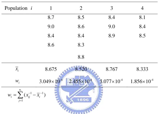
Example 2

The second data set is taken from Tweedie (1956) and has been used by Seshadri (1999, p.175) to perform the ANORE. The data set consists of four unbalanced populations and is modeled via the IG distribution. When λ_i’s are assumed to be the same for all groups, the P-value is 0.1879 for testing equality of four IG means through the analysis of reciprocals method. Therefore, we can use the

proposed method to construct the confidence interval for the common mean parameter. The data and the interval estimation are given in tables 7 and 8. Table 7 shows that when the data are homogeneous, the point estimators and confidence intervals for three methods are quite similar.

Table 7 Population i 1 2 3 4 8.7 8.5 8.4 8.1 9.0 8.6 9.0 8.4 8.4 8.4 8.9 8.5 8.6 8.3 8.8 i x 8.675 8.520 8.767 8.333 i w -4 3.049 10× 2.455 -4 10 × 3.077 -4 10 × 1.856 -4 10 × 1 1 1 ) ( i n i ij j i x w x− = − =

∑

−

Table 8 : The 95% confidence intervals for the common mean method Point estimate μ ˆ Interval estimate

*

r 8.56 (8.353, 8.789)

r 8.56 (8.407, 8.718)

5. Conclusions

In this thesis, we presented an accurate higher order likelihood-based procedure to construct the confidence interval of the common mean of several independent IG populations. In our simulation, we compared this procedure with two alternative methods with respect to their coverage probabilities, average lengths and type I errors. The numerical examples showed that the proposed method gives nearly exact coverage probability and the type I errors are close to the nominal level .05 even for small sample size. The method is able to integrate the information of several non-homogeneous IG populations, and therefore is useful for a variety of practical applications.

References

Barndorff-Nielsen, O.E., 1986. Inference on full and partial parameters based on the standardized signed log likelihood ratio. Biometrika 73, 307-322.

Barndorff-Nielsen, O.E., 1991. Modified signed log-likelihood ratio. Biometrika 78, 557-563.

Barndorff-Nielsen, O.E., Cox, D.R., 1994. Inference and asymptotics. Chapman & Hall, London.

Chhikara, R.S., Folks, J.L., 1989. The inverse Gaussian distribution. Marcel Dekker, New York.

Cox, D.R., Hinkley, D.V., 1974. Theoretical statistics. Chapman & Hall, London. Fraser, D.A.S., Reid, N., Wu, J., 1999. A simple general formula for tail probabilities

for frequentist and Bayesian inference. Biometrika 86, 249-264.

Lancaster, T., 1972. A stochastic model for the duration of a strike. Journal of the Royal Statistical Society A135(2), 257-271.

Mudholkar, G. S., Tian, L., 2002. An entropy characterization of the inverse Gaussian distribution and related goodness-of-fit tests. Journal of Statistical Planning and Inference 102, 211-221.

Reid, N., 1996. Likelihood and higher-order approximations to tail areas: A review and annotated bibliography. Can. J. Statist. 24, 141-166.

Seshadri, V., 1999. The Inverse Gaussian distribution: Statistical Theory and Applications. Springer, New York.

Thomas, A.S., 1999. An empirical adjustment to the likelihood ratio statistic Biometrika 86, 235-247.

Tian, L., Wilding, G.E., 2005. Confidence interval of the ratio of means of two independent inverse Gaussian distributions. Journal of Statistical Planning and Inference 133, 381-386.

Tian, L., 2005. Testing equality of inverse Gaussian means under heterogeneity based on generalized test variable. Computational Statistics & Data Analysis 51, 1156-1165.

Tweedie, M.C.K.,1941. A mathematical investigation of some electrophoretic measurements on colloids. Unpublished M.Sc. Thesis, University of Reading, England.

Tweedie, M.C.K.,1945. Inverse statistical variates. Nature, 155, 453.

Tweedie, M.C.K.,1946. The regression of the sample variance on the sample mean. Journal of London Mathematical Society. 21, 22-28

Tweedie, M.C.K.,1947. Functions of a statistical variate with given means, with special reference to Laplacian distributions. Proceedings of the Cambridge Philosophical Society 43, 41-49

Tweedie, M.C.K., 1956. Some statistical properties of inverse Gaussian distributions. Virginia Journal of Science 7, New Series, 160-165.

Tweedie, M.C.K, 1957. Statistical properties of inverse Gaussian distributions-Ⅰ. Annals of Mathematical Statistics 28, 362-377.

Tweedie, M.C.K, 1957. Statistical properties of inverse Gaussian distributions-Ⅱ. Annals of Mathematical Statistics 28, 696-705.

Wise, M. E., 1971. Skew probability curves with negative powers of time and related to random walks in series. Statistica Neerlandica 25, 159-180.

Wise, M. E., 1975. Skew distributions in biomedicine including some with negative powers of time in statistical distributions in scientific work. Vol. 2, D. Reidel, Dordrecht, Holland.

Wise, M. E., Osborn, S. B., Anderson, J., and Tomlinson, R. W. S., 1968. A stochastic model for turnover of radiocalcium based on the observed laws. Mathematical Biosciences 2, 199-224.

Wu, J., Jiang, G., Wong, A.C, Sun, X., 2002. Likelihood analysis for the ratio of means of two independent log-normal distributions. Biometrics 58(2), 463-469. Wu, J., Wong, A.C.M., Jiang, G., 2003. Likelihood-based confidence interval for a

log-normal mean. Statistics in Medicine 22, 1849-1860.

Wu, J., Wong, A.C.M., 2004. Improved interval estimation for the two-parameter Birnbaum-Saunders distribution. Computational Statistics & Data Analysis 47, 809-821