微聚焦端泵浦掺釹釩酸釔雷射在簡併共振腔下的動態與穩態行為

全文

(1)國立交通大學光電工程研究所博士論文. 微聚焦端泵浦掺釹釩酸釔雷射在簡併共振腔下的動態與穩態行為 Dynamics and stability behaviors in tightly focused end-pumped Nd:YVO4 laser around the degenerate cavity configurations. 研究生 : 戴伯澤指導教授 : 謝文峰教授吳小華教授. 中華民國九十四年六月.

(2) 微聚焦端泵浦掺釹釩酸釔雷射在簡併共振腔下的動態與穩態行為 Dynamics and stability behaviors in tightly focused end-pumped Nd:YVO4 laser around the degenerate cavity configurations. Student: Po-Tse Tai Advisor: Wen-Feng Hsieh Hsiao-Hua Wu. 研究生: 戴伯澤指導教授: 謝文峰吳小華. 國立交通大學光電工程研究所博士論文. A Thesis Submitted to the Department of Photonics & Institute of Electro-Optical Engineering College of Electrical Engineering and Computer Science National Chiao Tung University in partial Fulfillment of Requirements for the Degree of Doctor of philosophy in Electro-Optical Engineering. June 2005 Hsinchu, Taiwan, Republic of China. 中華民國九十四年六月.

(3) 誌謝從小到大的求學歷程中，只有攻讀博士的階段不知道是否可以或是何時可以畢業。在這一段漫長的過程中，所得到的經驗是非常寶貴的。學位的取得不只是帶來喜悅而且也帶來了自我的肯定，這些心境的改變勢必會在往後的日子慢慢的醞釀。在這段期間非常感謝指導老師謝文峰教授在研究態度與精神上的鍛鍊，以及吳小華教授在實驗技巧上的指導，使我能夠具備該有的技能。也非常感謝與我合作非常密切的陳慶緒學長，因為數值模型的建立使得我的實驗能有更完善的解釋。對於兩個跟我ㄧ起做實驗的學弟李國昶與邱偉豪，也非常感謝你們的努力讓我有多餘的時間，可以擴展實驗的方向與技巧，在這也祝福你們有美好的將來。幸運的在我博士班最後的兩年半讓我遇到了珮芳。使我在低潮的時候能夠樂觀的面對，遇到瓶頸時能夠給我突破的靈感。最重要的，妳也能夠和我ㄧ起分享生命裡的喜悅，希望我們能夠永遠的扶持對方下去。感謝這段期間遇到的所有人，你們給了我一個難忘的回憶。感謝國科會計畫 NSC93-2112-M-009-035 所提供的獎學金以及實驗的經費讓我能夠順利的完成所有的研究。.

(4) 微聚焦端泵浦掺釹釩酸釔雷射在簡併共振腔下的動態與穩態行為. 學生: 戴伯澤. 指導老師: 謝文峰教授吳小華教授. 國立交通大學光電工程學系. 摘要. 我們研究一個操作在 1/3 簡併共振腔附近與小聚焦端泵浦的掺釹釩酸釔雷射，其共振腔結構相關的動態行為。強烈聚焦的泵浦光線會因為熱透鏡的效果，而產生巨大的相位變化進而影響共振腔的結構。為了讓數值模擬能夠符合實驗的結果，我們將熱透鏡的效應加入數值模擬。數值模擬可以指出哪些位置可以產生自脈衝的現象，為什麼我們可以在長短不同共振腔下觀察到時-空不穩脈衝現象，以及只有時間不穩定脈衝，這些結果都跟實驗非常的符合。除了在長腔的不穩區域之外，我們實驗上也觀察到橫模的光頻鎖定，及無橫模拍頻。利用基因演算法計算模態展開時，每個模態的振幅權重以及相對的相位，我們發現在完全簡併的共振腔下所有的橫模都是同相位。即使我們調離開簡併共振腔，所有的橫模還是保有相位與光頻的鎖定。即便調離簡併共振腔大約 1mm，我們仍可以觀察到模形(beam profile)會隨著傳播方向改變，這是由於所有的橫模在一開始就是相位鎖定。由於在簡併共振腔下所有的橫模會保有光頻與相位的鎖定，我們可以利用這個特性來控制雷射的模形。我們驗證了在一個小聚焦與端泵浦的掺釹釩酸釔雷射可以直接產生多樣的瓶型光束。只要適當的控制泵浦 I.

(5) 光斑與腔內實光欄的大小，在半共焦腔、1/3 簡併腔、與 1/5 簡併腔下可以產生不同但是對比度極佳的瓶型光束。這樣的新發現是適用於內含任意增益介質之小聚焦端泵浦雷射。這樣的雷射也可抑制空間燒洞(spatial hole burning)效應。由於雷射模會自動調整大小以符合泵浦光斑，雷射可以在被幫浦增益介質區域內達到很高的光強度，而使得大部分的增益被高強度的駐波消耗掉。我們利用一個縱向相關的速率方程式來描述與研究這個在平凹共振腔掺釹釩酸釔雷射的實驗。即使高於 20 倍的閥值，實驗上我們可發現這個抑制空間燒洞的效應。. II.

(6) Dynamics and stability behaviors in tightly focused end-pumped Nd:YVO4 laser around the degenerate cavity configurations. Student: Po-Tse Tai. Advisor: Professor Wen-Feng Hsieh Professor Hsiao-Hua Wu. Department of Photonics and Institute of Electro-Optical Engineering National Chiao Tung University. Abstract. We experimentally and numerically studied cavity-dependence of laser dynamics in an tightly-focused end-pumped Nd:YVO4 laser which operates in the vicinity of 1/3-degenerate cavity.. The tightly-focused pump beam. results in enormous phase distortion which influences the cavity configuration through the thermal lens effect, therefore, the thermal lens effect is considered in our simulation.. The simulation results well explain. our experimental observation including the regions of self-pulsation, the reasons why we should observe the temporal or the spatiotemporal dynamics in the instability region on short- or long-cavity side of the degeneracy, and the influence of thermal lens. In addition, the transverse modes are all frequency-locked over the cavity tuning except for the instability regions. By decomposing the calculated mode (similar to the observed one) into the degenerate transverse modes to obtain their mode weights and relative phases, we found that the transverse modes are all in phase at the exactly degenerate cavity.. Except for the cavity configuration within the instability III.

(7) region on the long cavity side, all of the transverse modes are phase- and frequency-locked to one another even when the cavity is tuned away from the degeneracy.. This finding consists with the experimental observation. that the stationary transverse mode pattern does vary along the propagation axis due to interfere of Guoy phases from the phase-locked transverse modes even for cavity length being adjusted 1mm away from the degeneracy. Because the transverse modes which govern the laser pattern are in-phase and frequency-locked at the degeneracy, we should be able to control the laser pattern. We demonstrate various optical bottle beams can be directly generated from a tightly focused end-pumped Nd:YVO4 laser. By controlling the size of pump beam and inserting an intracavity aperture in the plano-concave cavity, we obtain good contrast optical bottles at semi-confocal, 1/3-, and 1/5-degenerate cavity configurations, respectively. This new observation is universal that is suitable for any kinds of gain media in tightly end-pumped lasers. We also found that the spatial hole-burning effect can be suppressed in this laser. Due to shrinkage of the beam waist of laser mode to match the pump beam, this laser can attain very high intensity in the pump region of gain medium and therefore most of its gain is depleted even by a standing wave.. This was demonstrated by a simulation with spatial dependent rate. equations and experiment results of a plano-concave Nd:YVO4 laser. The suppression effect was observed up to 20 times the pump threshold.. IV.

(8) Table of contents. 摘要 ................................................................................................................. I ABSTRACT................................................................................................. III TABLE OF CONTENTS.............................................................................. V LIST OF FIGURES ...................................................................................VII CHAPTER 1 INTRODUCTION..................................................................1 1.1 GEOMETRICAL STABLE CONDITION..........................................................1 1.2 DEGENERATE CAVITIES AND ITERATIVE MAP ...........................................2 1.2-1 Resonance frequencies and degenerate cavities ............................2 1.2-2 Iterative map...................................................................................4 1.3 LASER PATTERNS IN DEGENERATE CAVITY ...............................................7 1.4 AIMS OF THIS RESEARCH .......................................................................10 REFERENCES ...............................................................................................13 CHAPTER 2 SIMULATION MODEL FOR OUR LASER SYSTEM...14 2.1 HUYGENS’S INTEGRAL AND ABCD MATRIX ..........................................14 2.1-1 Huygens’s integral ........................................................................14 2.1-2 Relationship between ABCD matrix and Huygens’s integral.......15 2.2 SIMULATION MODEL IN A LASER CAVITY ................................................17 2.3 THERMAL LENS AND MODIFICATION OF SIMULATION MODEL .................20 2.4 CONCLUSION .........................................................................................22 REFERENCES ...............................................................................................24 CHAPTER 3 LASER DYNAMICS AROUND 1/3-DEGENERATE CAVITY ........................................................................................................25 3.1 INTRODUCTION .....................................................................................25 3.2 EXPERIMENT SETUP...............................................................................26 3.3 EXPERIMENTAL RESULTS AND DISCUSSIONS ..........................................27 3.3-1 Locations of spontaneous instability ............................................27 3.3-2 Laser dynamics in instability region ............................................32 3.3-3 Cooperative frequency locking and laser patterns.......................42 3.4 CONCLUSION .........................................................................................49 V.

(9) REFERENCES ...............................................................................................50 CHAPTER 4 LASER PATTERNS AROUND DEGENERATE CAVITY: OPTICAL BOTTLE BEAMS.....................................................................52 4.1 MOTIVATION .........................................................................................53 4.2 EXPERIMENT SETUP AND DISCUSSION ....................................................57 4.3 CONCLUSION .........................................................................................64 REFERENCES ...............................................................................................65 CHAPTER 5 OPTICAL SPECTRUM AROUND THE DEGENERATE CAVITY: SUPPRESSION OF SPATIAL HOLE BURNING ...............66 5.1 THEORETICAL MODEL AND SIMULATION ................................................67 5.2 EXPERIMENT SETUP AND RESULTS .........................................................71 5.3 CONCLUSION .........................................................................................77 REFERENCES ...............................................................................................79 CHAPTER 6 CONCLUSION AND FUTURE WORKS..........................80 6-1 LASER DYNAMICS .................................................................................80 6.2 LASER LINEWIDTH ................................................................................82 6.3 OPTICAL TRAPPING ...............................................................................83 REFERENCES ...............................................................................................84. VI.

(10) List of Figures. Fig. 1-1 The diagram of residue versus g1g2............................................................................6 Fig. 1-2 The sketch of multipass transverse mode at 1/3-degenerate cavity............................9 Fig. 1-3 Propagation of the multi-beam waist mode. ..............................................................9 Fig. 2-1 The sketch of one-dimension Huygens’s integral.. ...................................................15 Fig. 2-2 The sketch of the optical ray through an ABCD paraxial system.............................17 Fig. 2-3 The sketch of plano-concave cavity..........................................................................19 Fig. 2-4 Side view and end view of an applicable laser rod and heat sink.. ..........................21 Fig. 3-1 The schematic experimental set up.. ........................................................................27 Fig. 3-2 The observed output power as a function of cavity length and the unstable regions in terms of the cavity length and the pump power for different pump spot (wp)....29 Fig. 3-3 The numerical output power as a function of cavity length with considering the thermal lens effect and the unstable regions for different wp................................31 Fig. 3-4 The numerical output power as a function of cavity length and the unstable regions without considering the thermal lens effect...........................................................32 Fig. 3-5 The far-field mode patterns inside the long-cavity unstable region and inside the short-cavity unstable region..................................................................................33 Fig. 3-6 The temporal evolution of laser output. ...................................................................35 Fig. 3-7 The recording time traces of temporal and special-temporal..................................37 Fig. 3-8 (a) A self-pulsing temporal evolution of the simulated output power without the thermal lens effect for M=5.96 cm. (b) The normalized intensity profiles and their corresponding far-field profiles (inset) from the pulse peak (solid circles). (c) The numerical temporal evolution of the output power in the vicinity of the degeneracy with the thermal lens effect for L=6.005 cm. (d) The intensity profiles and their corresponding far-field profiles (inset) of three successive round trips.............................................................................................................39 Fig. 3-9 The time evolution of self-pulsation by 10 times scaling..........................................42 Fig. 3-10 The intensity profile in logarithm scale and the phase profile at different cavity length.. ..................................................................................................................46 VII.

(11) Fig. 3-11 The mode weightings and the relative phases of the LGp0 modes as L!are tuned away from the degeneracy. ...................................................................................47 Fig. 3-12 (a) The numerical beam profile variation along the propagation distance. (b) The photograph experimentally taken at 20.5 cm after the convergent lens.........48 Fig. 4-1 Intensity patterns and their corresponding three-dimension profiles.......................55 Fig. 4-2 The transverse modes distribution as well as overlap integral of pump spot (Wp) and W0...................................................................................................................56 Fig. 4-3 The sketch of experiment setups...............................................................................58 Fig. 4-4 The radial intensity patterns of the optical bottle generated from a laser operated with the 1/4-degenerate cavity at various distances from the transform lens. ......59 Fig. 4-5 The calculated radial intensity distributions and the experimentally observed beam profiles.. ................................................................................................................61 Fig. 4-6 The depth of optical bottle versus different pumping size and corresponding calculated profiles at 1/5-degeneracy. ..................................................................62 Fig. 4-7 Photographs of the far-field patterns by the laser operated at semi-confocal, 1/3, and 1/5 degenerate configurations........................................................................63 Fig. 5-1. Numerical spatial distribution of steady-state upper level density to show influence of spatial hole-burning effect. ...............................................................................70 Fig.5-2 The sketch of experiment setups................................................................................72 Fig. 5-3 Single frequency optical spectrum of the Fabry-Perot interferometer.....................73 Fig. 5-4 Typical multiple optical frequency and corresponding RF spectrum for the common laser at L=6.06cm.................................................................................................74 Fig. 5-5 Multiple optical frequency and corresponding RF spectrum under 310mW pumping at g1g2=1/4. ...........................................................................................................77 Fig. 6-1 The relaxation oscillation versus normalization pumping power ............................81. VIII.

(12) Chapter 1 Introduction. A laser system must contain a pumping source, gain media, and optical resonator. The simplest kind of optical resonator consists of just two curved mirrors set up facing to each other. Simple two-mirror cavities are widely used in practical lasers, and the properties of stable resonators are the basic lore of laser physics.. Although the paraxial optics can easily obtain a. geometrical stable condition, there are many dynamics and stability behaviors in some special cavity configurations [1-7]. In this study, we will focus on laser dynamics and stationary laser parameters dependent on its resonators.. 1.1 Geometrical stable condition Gaussian beams are the eigenfunctions of a laser resonator.. We can. use a complex q-parameter to represent a Gaussian beam of which the real and the imaginary parts respectively indicate the radius of curvature and the beam width.. The transformation rule of paraxial wave using the ABCD. matrix elements to relate the q-parameters as it propagates according to the so-called ABCD law as. q2 =. Aq1 + B , Cq1 + D. (1.1). where q1 is the initial state of Gaussian beam and q2 is the final state after Gaussian beam propagates through a paraxial optical system characterized by the ABCD matrix.. Let the elements of ABCD matrix in Eq. (1.1) be those. for a round trip of the laser cavity.. Thus, q1 will equal to q2 because the 1.

(13) laser beam should be self-consistent after propagating a round trip. Therefore we can solve the self-consitent q-parameter qs as 2 ⎤ ⎡ A− D ⎛ A+ D ⎞ ⎥ ⎢− ± i 1− ⎜ ⎟ 2 ⎢ ⎝ 2 ⎠ ⎥ ⎣ ⎦. qs = B. (1.2). For ensuring qs be a complex number, we obtain the criterion of a stable cavity:. A+ D ≤ 1. 2. (1.3). Assume two mirrors which form a resonator having radii of curvature of R1 and R2 are separated by L, the round trip elements of ABCD matrix are trivial to obtain and substitute into Eq. (1.3) and the stable condition of optical resonator becomes. 0 ≤ g1 g 2 ≤ 1 , where g1, 2 = 1 − L. R1, 2. (1.4) .. This stability criterion of Eq. (1.4) is suitable for. any two-mirror optical resonator and is called the geometrically stable condition. However, we only consider the geometrically stable condition for a real laser cavity is not enough if there are additional effects that can result in instability output of laser, and we will discuss it as follows.. 1.2 Degenerate cavities and iterative map. 1.2-1 Resonance frequencies and degenerate cavities. The resonance condition for a standing-wave cavity is that the phase shift for total round-trip must be an integer multiple of 2π.. The total phase. shift from one end of cavity to the other end includes kL and Gouy phase 2.

(14) shift terms, where k = 2π. λ is the wave number, λ is wavelength of laser,. and the Gouy phase is an additional phase introduced by a paraxial wave function substitution for an (n,m)-th order Hermite-Gaussian mode in mathematics. The total Gouy phase shift of a laser cavity with resonator length L is given in terms of the g-parameters by the formula. ( n + m + 1) cos −1 (±. g1 g 2 ) ,. (1.5). where n and m are the mode numbers in the x- and y-axes, respectively. Because the Gouy phase shift depends on Hermite-Gaussian mode number, different transverse modes of a stable Gaussian resonator have different resonance frequencies and the resonance frequency of Hermite-Gaussian (n,m) mode is therefore given by. ν n , m, q =. c ⎛ m + n + 1 −1 ⎞ cos g1 g 2 ⎟ , ⎜q + 2L ⎝ π ⎠. (1.6). where q is the longitudinal mode number. Form Eq. (1.6), we can define νl=c/2L is the longitudinal mode spacing, and νt=(νl/π)arcos[(g1g2)1/2] is the. transverse mode spacing. The configurations with g1g2= 0, 1/4, and 1/2 correspond to ν  t/νl= 1/2, 1/3, and 1/4, respectively, therefore, we denote them as 1/2-, 1/3-, 1/4-degenerate configurations. In these configurations, the fundamental modes may be degenerate with other high-order transverse modes which obey Eq. (1.6). The degenerate modes may through the mode competition or the mode beating result in instability of laser output [8-9]. Therefore, we know the degenerate cavity is a good choice to investigate laser dynamics.. 3.

(15) 1.2-2 Iterative map. The iterative map is a mathematical tool to realize the dynamic behaviors in a physical system. This method use discrete time system to study a continuous system.. Applying the ABCD matrix for a lossless. two-mirror resonator, we can define a two-dimension iterative map which contains the spot size w and radius of curvature R as below [2] 2 2 ⎧ ⎪ w n +1 = h(R n , w n ) = w n ⎛⎜ A + B ⎞⎟ + ⎛⎜ λ 2 ⎞⎟ B 2 R n ⎠ ⎝ πw n ⎠ ⎝ ⎪ ⎪⎪ 2 2 ⎞ 2 ⎛A + B ⎞ +⎛ λ . ⎨ ⎜ ⎟ ⎜ 2⎟ B R π w ⎪ n⎠ ⎝ n⎠ ⎝ 2 ⎪R n+1 = f (R n , w n ) = ⎞ ⎛ A + B ⎞⎛ C + D ⎞ + ⎛ λ ⎪ BD ⎜ R n ⎟⎠⎜⎝ R n ⎟⎠ ⎜⎝ πw 2n ⎟⎠ ⎪⎩ ⎝. (1.7). The suffix of n represents the round-trip index where A, B, C, and D are elements of the round-trip matrix, and the discrete time interval of the map is equal to one round-trip time of the resonator. Under linear stability analysis, the stability of fixed point is determined by its Jacobian eigenvalue of the map. The fixed point is the self-consistent solution of q-parameter, i.e., the steady-state solution. Therefore discussing the Jacobin eigenvalue at fixed point is equivalent to determine the dynamic stability of laser resonator. Because the map belongs to conserve system, the determinant of Jacobian matrix equals to unity and the eigenvalue of Jacobian matrix depend on its trace. For convenience, we use the residue to discuss the stability condition which is defined as. Res =. 1 [2 - Tr (M J )] , 4. (1.8). where MJ is the Jacobian matrix and Tr(MJ) is its trace. When 0<Res<1, the eigenvalues are complex with unity magnitude and the system is stable, 4.

(16) whereas the system is unstable with either Res<0 or Res>1. In the standing wave resonators with real round-trip transfer matrices, the curvature of laser beam must match the end mirrors. Therefore, by substituting the the trace of Jacobin derived from the round-trip transfer matrix into Eq. (1.8), we have the residue 2. 2 Res = 1 - ⎛⎜ A + B ⎞⎟ = 1 - (2G1G 2 - 1) . R 1⎠ ⎝. (1.9). Here we have defined G1=a-b/R1 and G2=c-d/R2 as the G-parameters for general optical resonators, and a, b, c, and d are the elements of transfer matrix of single pass between the two end mirrors.. We can use. G-parameters to discuss the stability of a multi-element resonator. For simplicity, we discuss the stability by a two-mirror resonator. Thus ⎡1 L⎤ the single pass transfer matrix is ⎢ ⎥ and ⎣0 1 ⎦. Res = 1 - (2g1g 2 - 1) , 2. where g1,2 = 1 - L. R1,2. (1.10). and the definition of g-parameters are the same as in. Eq. (1.4). From Eq. (1.10), we found that the residue is a function of g1g2 only. A plot of the diagram of residue versus g1g2 is presented in Fig. 1-1. Since the resonator is dynamically unstable for Res<0 or Res>1, in Fig. 1-1, one gets a region with g1g2<0 or g1g2>1. And the dynamic stable region with 0<Res<1 is also geometrically stable corresponding to 0<g1g2<1. It is critical stable for Res=0 with g1g2=0 or g1g2=1. The stable region of residue theorem is the same as the geometrical stability ones which has been discussed in Section 1.1. However, another critical stable point at g1g2=1/2 with Res=1 in Fig. 1-1 can not be found by using the paraxial optics. 5.

(17) Stability region decided by the iterative map of the beam parameters provides not only geometrical stable condition but also dynamically critical stable condition.. 1.0. Residue. 0.8 0.6 0.4 0.2 0.0 0.0. 0.2. 0.4. 0.6. 0.8. 1.0. g1g2 Fig. 1-1 The diagram of residue versus g1g2. It can easily be observed that the stable region of the residue is the same as geometrical stable condition.. From the residue theorem, these special cases with Res = 0, 1, 3/4, and 1/2 correspond to the low-order resonance where p=1, 2, 3, and 4 satisfying χp=1, respectively.. Here χ is the eigenvalue of MJ.. Under these. circumstances, the complicated dynamics may occur at these configurations if there is a persistent nonlinear effect. These special conditions correspond to g1g2=0 or g1g2=1 for Res=0; g1g2=1/2 for Res=1; g1g2=1/4 or g1g2=3/4 for. (. ). Res=3/4; and g1g2= 2 ± 2 /4 for Res=1/2, respectively [1-2]. It is worth noting that these configurations correspond to degenerate cavities and these degenerate cavities are very sensitive to any perturbation in the laser system. Therefore if any nonlinear effect is in a laser system, the laser will present various. dynamics. behavior.. In. the. previous. study. [10],. the. cavity-dependent laser dynamics has been studied in a Kerr-lens mode locked 6.

(18) (KLM) Ti-sapphire laser. When the optical Kerr effect was considered as the nonlinear dynamical parameter, optical bistability and multiple-period bifurcation were numerically demonstrated.. 1.3 Laser patterns in degenerate cavity Even now except for a few special situations, rigorous mathematical existence and completeness proofs for optical resonator eigenmodes do not exist.. Because the conventionally laser cavity is an open-side optical. resonator, the laser is not a lossless system. Real lasers have never had any difficulty in finding eigenmodes.. Empirical and experimental evidence. show the same results of lossless system, such as microwave cavities or microwave waveguide, the eigenmodes of laser resonator exist. Therefore, the concept of eigenmodes, such as the Laguerre-Gaussian or the Hermite-Gaussian mode, has long time been accepted and provides a physically realistic and meaningful basis for describing laser resonator in real system. In ray analysis of the resonators, however, a paraxial resonance equation [11] yields the mirror separations of a two-mirror cavity in which any arbitrary rays repeat themselves after an integer number (say N) of return transits. It has been argued that a set of paraxial closed ray paths that is complete in N round trips might also be regarded as a mode of the resonator. By investigating the effects of off-axis pump on the laser with these degenerate resonator configurations [12], it can be found that a symmetric pattern forms for even N and an asymmetric pattern forms for odd N. These results may be accounted for simply by the introduction of multipass 7.

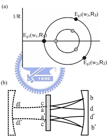
(19) transverse (MPT) modes that self-reproduce after several round trips in terms of the ray matrix analysis but not by the superposition of standard cavity modes. In the recently study of multi-beam waist mode [13], we can use propagation of Gaussian q-parameter at 1/3-degenerate cavity to realize multipass transverse mode as showed in Fig. 1-2. In accordance with Fig. 1-2(a), in Fig. 1-2(b) we depict the Gaussian-beam evolution in which the first round-trip wave begins with Eg1 (w=aa’/2, R1= ∞ ) and reproduces itself after three round trips in the cold cavity. Note that a positive R represents a divergent wave riding in the propagation direction. The second round trip begins when Eg2(w2=cc’/2, R2) converges at dd’ owing to negative R2; which means that the light wave emanates from Eg2 just as from dd’. The third round trip, with Eg3(w3=w2 , R3=-R2), is divergent from cc’; however, it seems to emanate from dIdI’.. As discussed above, it implies that the. locations of aa’, dd’, and dIdI’ are point sources, respectively, therefore it can be expected that three beam waist can be observed after focusing this laser mode. If we place a transform lens with a focal length of 5.2 cm a distance of 10.5 cm from a plano-concave cavity which operated at 1/3-degenerate cavity with cavity length of 6cm, this is equivalent to propagating a distance of 16.5 cm from the flat mirror and then through the transform lens. Therefore, three point sources at dd’, aa’, and dIdI’, in the Fig. 1-2 (b), have distances of 10.5cm, 16.5cm, and 22.5cm from the transform lens respectively. An image formula of Gauss is used to determine the locations of images, as a result, three images are located at 10cm, 7.8cm, and 6.8cm, 8.

(20) respectively. A charge-coupled device (CCD) directly images the mode pattern behind the transform lens and in order to reduce the noise, a laser line filter was placed in front of the camera lens of CCD. The images according with distance are shown in Fig. 1-3. It is clearly that the experiment results fit with the calculation of geometric optics and the model of multipass transverse mode.. (a) Eg3(w3,R3). 1/R Eg1(w1,R1). . Eg2(w2,R2). (b). dI dI＇. b. c a a＇ c＇. d d＇ b＇. Fig. 1-2 The sketch of multipass transverse mode at 1/3-degenerate cavity. (a) Periodic orbits of the q-parameter for the empty cavity. The two concentric circles mean that there are infinite sets of period-N solutions. (c) Gaussianbeam evolution in the empty cavity.. Z=6.8cm. 7cm. 7.8cm. 8cm. 9cm. Fig. 1-3 Propagation of the multi-beam waist mode. 9. 10cm.

(21) In fact, the multi-beam waist made can be explained as a supermode [14-15].. The supermode is superposed by many high-order degenerate. transverse modes, and because of cooperative frequency locking of the degenerate modes the laser pattern is temporal stationary. In addition, the pattern propagating in free space along the beam axis is not stationary due to the interference of the degenerate modes. The concept of eigenmodes also can well explain the experiment results, although it needs a serial of calculation but not an intuitional process. Nevertheless, it is interesting that a complicated problem of wave optics can be simplified to a geometrical optics one.. 1.4 Aims of this research In this research, we will investigate the laser dynamics under stationary laser parameters in a simple plano-concave tightly-focused end-pumped Nd:YVO4 laser near the degenerate resonators, and a model of Huygens’s integral together with the rate equations will help us to analyze this laser system. We found that the laser instability occurs in a very narrow range of cavity tuning on each side of the degeneracy points that shows periodic, period-doubling, and chaotic time evolutions.. In our experiment, an. extremely small wp will increase the mode weights of the high-order degenerate modes to as much as the fundamental Gaussian mode. Although so many degenerate modes which bring a supermode join to laser instabilities, the dynamic behaviors on short-cavity side are only temporal instabilities, the instabilities on the long-cavity side are spatiotemporal which results from the 10.

(22) nonlinear coupling between the supermode and the other Laguerre-Gaussian modes.. From the simulation model, we found that the other. Laguerre-Gaussian modes are introduced by the thermal lens effect. It is the first time to discuss the relationship between the laser instability and thermal lens effect. Under tightly-focused pumping, the supermode is formed around the degenerate cavity. We utilize the supermode to directly generate various optical bottle beams at different degenerate cavities. An optical bottle beam has a low-intensity zone surrounded by a high intensity shell that can be applied to trap low-index micro-particles or blue-detuned atoms. Optical bottle beams had been generated in the use of holograph, spatial light modulator, and two-beam interference.. Those methods need enormous. calculation to prepare a suitable holograph with low conversion efficiency or well control of phase retardation for each pixel of SLM and two overlapped beams to make the destruction interference occurring at the beam center. Our method of generating bottle beams directly from a simple laser is convenient for various applications. We will also investigate the spectrum of laser at degenerate cavities. In a standing wave resonator, the spatial hole-burning effect can be suppressed. This laser can attain very high intensity in the gain medium due to shrinkage of its beam waist to match the pump beam and therefore most of its gain is depleted even by the standing wave. This experimental result proves a useful method to control the mode selection in this degenerate cavity, instead of using otherwise additional dispersion components such as filters or gratings. 11.

(23) In this dissertation, it will introduce the simulation model which includes how the thermal lens effect substitutes or modifies the model in Chapter 2. And than we will discuss our experimental results which are laser dynamics in Chapter 3, directly generation of optical bottle beam in Chapter 4, and optical spectrum of around degenerate cavity in Chapter 5.. Finally, in. Chapter 6 it will state the conclusions and then give suggestions for future work.. 12.

(24) References [1]. M.D. Wei and W.F. Hsieh, J. Opt. Soc. Am. B 17, 1335 (2000). [2]. M.D. Wei, W.F. Hsieh, and C. C. Sung, Opt. Commu. 146, 201 (1998). [3]. Y.F. Chen and Y.P. Lan, Phys. Rev. A 63, 063807 (2001). [4]. C.H. Chen, M.D. Wei and W.F. Hsieh, J. Opt. Soc. Am. B 18, 1076 (2001). [5]. P. Laporta and M. Brussard, IEEE J. Quantum Electron. 27, 2319 (1991). [6]. H. H. Wu and W. F. Hsieh, J. Opt. Soc. Am. B 18, 7-12 (2001). [7]. V. Couderc, O. Guy, A. Barthelemy, C. Froehly, and F. Louradour, Opt. Lett. 19, 1134 (1994). [8]. L. A. Lugiato, G. L. Oppo, J. R. Tredicce, L. M. Narducci, and M. A. Pernigo, J. Opt. Soc. Am. B 7, 1019 (1990). [9]. J. R. Tredicce, E. J. Quel, A. M. Ghazzawi, C. Green, M. A. Pernigo, L. M. Narducci, and L. A. Lugiato, Phys. Rev. Lett. 62, 1274 (1989). [10]. J. H. Lin, M. D. Wei, and W. F. Hsieh, J. Opt. Soc. Am. B 18, 1069 (2001). [11]. Ramsay and J. J. Degnan, Appl. Opt. 9, 385 (1970). [12]. E. Siegman, Laser (Mill Vally, CA, 1986). [13]. C. H. Chen, P. T. Tai, W. F. Hsieh, and M. D. Wei, J. Opt. Soc. Am. B 20, 1220 (2003). [14]. C. H. Chen, P. T. Tai, W. H. Chiu, and W. F. Hsieh, Opt. Commu. 245, 301 (2005). [15]. L. A. Lugiato, G. L. Oppo, M. A. Pernigo, J. R. Tredicce, and L. M. Narducci, Opt. commun. 68, 63 (1988). 13.

(25) Chapter 2 Simulation model for our. laser system. Fox and Li approach [1-3] is usually used to elucidate the physical picture of radiation in an optical resonator, which repeatedly circulates around the cavity that contains a thin slab gain medium.. The transverse. mode profile can be calculated based on the central laser wavelength because the diffraction effect experienced by transverse modes will be essentially the same for those any one of axial mode frequencies within the oscillation bandwidth.. In the numerical procedure, an arbitrary initial field will. eventually converge to a state which the mode profile will self-consistent after one round-trip. In our study [4], we use this approach to simulate an end-pumped solid-state laser.. 2.1 Huygens’s integral and ABCD matrix. 2.1-1 Huygens’s integral. In the classical optics, we can use Huygens’s integral to describe an optical field after a certain distance of diffraction. So we also can use Huygens’s integral to describe laser beam in a real resonator. In Fig. 2-1, it is a sketch of one-dimension Huygens’s integral, and it means that the optical field of plane Z2 interferes with all of the point sources of plane Z1. In one-dimension condition, the Huygens’s integral is 14.

(26) ~. u 2 ( x2 ) =. j ∞ ~ u1 ( x1 ) exp[ − jkρ ( x1 , x2 )]dx1 , Lλ ∫− ∞. ~. (2.1). ~. where the u1 ( x1 ) and u 2 ( x2 ) are respectively the wave functions of Z1 and Z2 plane, k is the wave number and λ is the wavelength of laser field. The ρ(x1,x2) is the distance of the arbitrary position vectors on the Z1 and Z2 planes. Therefore we can define ρ as. ρ ( x1 , x2 ) = L2 + ( x2 − x1 ) 2 ≈ L +. ( x2 − x1 ) 2 , 2L. (2.2). We can use Eq. (2.1) and (2.2) to calculate the diffraction of optical field.. ~ u1(x1). ~ u2(x2) X2. X1. Z1. Z. L. Z2. Fig. 2-1 The sketch of one-dimension Huygens’s integral. L is the ~. separation distance between plane of Z1 and Z2, the u1 ( x1 ) and ~. u 2 ( x2 ) are the wave function of each plane.. 2.1-2 Relationship between ABCD matrix and Huygens’s integral. We usually use the ABCD matrix to present a paraxial system, such as laser resonator. If we substitute the elements of ABCD matrix to Huygens’s integral, it will be very convenient for using. Now, we will find the relationship between ρ(x1,x2) and ABCD matrix, and substitute to Huygens’s integral. In Fig. 2-2, a paraxial optical system between the plane of Z1 and Z2 can be expressed as 15.

(27) ⎡ x2 ⎤ ⎡ A B ⎤ ⎡ x1 ⎤ ⎢ x ' ⎥ = ⎢C D ⎥ ⎢ x ' ⎥ , ⎣ 2⎦ ⎣ ⎦⎣ 1 ⎦. (2.3). where the x and x’ respectively represent the positions and slopes of the ray on the Z1 and Z2 planes. From the Eq. (2.3), we can get the slope of each point as x2 − Ax1 B . Dx2 − x1 ' x2 = B. x1' =. (2.4). The input ray may be viewed as a ray coming from an object point P1 located a distance R1 behind the input plane, as shown in Fig. 2-2. Hence R1 and R2 is given by R1 x1 Bx1' ≡ ' = n1 x1 x2 − Ax1 R2 x2 Bx2' ≡ ' = n2 x2 Dx2 − x1. .. (2.5). Fermat’s principle says that “all rays connecting two conjugate points must have the same optical path length between two points.” Therefore the ray path from P1 to P2 through x1 and x2 will equal to the ray path along the optical axis ( P1 P2 = P1 x1 x2 P2 ). Both ray paths can be written as P1 P2 = n1 R1 + L0 − n2 R2 P1 x1 x2 P2 = n1 ( R12 + x12 )1 / 2 + ρ ( x1 , x2 ) − n2 ( R22 + x22 )1 / 2 . ≈ n1 ( R1 +. 2 1. (2.6). 2 2. x x ) + ρ ( x1 , x2 ) − n2 ( R2 + ) 2 R1 2 R2. From Eq. (2.6), we can get. ρ ( x1 , x2 ) = L0 +. 1 ( Ax12 − 2 x1 x2 + Dx22 ) . 2B. By substituting Eq. (2.7) into Eq. (2.1), the Huygens’s integral becomes 16. (2.7).

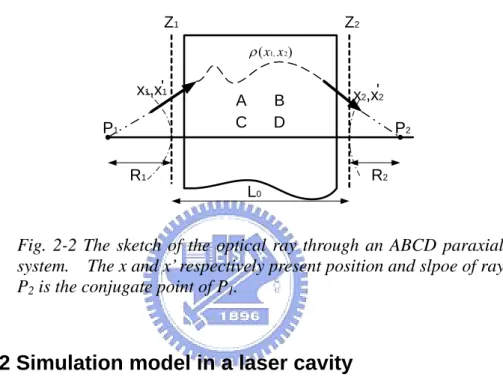
(28) ~. u 2 ( x2 ) =. ∞ ~ j π exp[ − jkL0 ]∫ u1 ( x1 ) exp[ − j ( Ax12 − 2 x1 x2 + Dx22 )]dx1 . − ∞ Bλ Bλ. (2.8) Therefore we have the relationship between elements of ABCD matrix and the Huygens’s integral.. Z1. Z2 ρ ( x1, x 2). x1,x'1 P1. A C. B D. R1. x2,x'2 P2 R2. L0. Fig. 2-2 The sketch of the optical ray through an ABCD paraxial system. The x and x’ respectively present position and slpoe of ray. P2 is the conjugate point of P1.. 2.2 Simulation model in a laser cavity Consider the plano–concave axially pumped solid-state laser shown in Fig. 2-3.. It consists of a laser crystal with one of its end faces. high-reflection coated as the flat mirror (M3) and a curved mirror (M2) with radius of curvature R as the output coupler which is separated by a distance L. Let the reference plane be the place of M1 where the light beam just leaves the laser crystal toward the curved mirror. As discussed previously, one can relate the one-dimension Huygens’s integral with the ABCD matrix. In this system, we need two-dimension Huygens’s integral. cylindrical symmetry, simplified formula can be obtained. 17. However, under.

(29) Em− +1 ( r ) =. j 2π exp[ j 2kL] ⎡ − jπ 2πrr ' ' ' + ' '2 2 ⎤ + E ( r ) exp ( Ar Dr ) J ( )r dr , m 0 ⎢ Bλ ∫ ⎥⎦ Bλ Bλ ⎣ (2.9). with the round-trip transmission matrix ⎡A B ⎤ ⎢ C D⎥ . ⎣ ⎦. (2.10). Here Em+ (r ' ) and Em− +1 ( r ) are the electric fields of the mth and the (m+1)st round trips on the planes immediately after and before the gain medium (denoted by the superscripts + and -), where r’ and r are the corresponding radial coordinates, λ is the wavelength of laser, and J0 is the Bessel function of zeroth order. In a thin-slab approximation, we can relate the electric fields E +m +1 to E -m +1 (after and before the gain medium) in the same round trip as. Em+ +1 ( r ) = Em− +1 ( r ) exp[σΔN m +1l ] × ρ × Π ( r / a ) ,. (2.11). where 1 - ρ 2 is the round-trip energy loss, σ is the stimulated-emission cross section, ΔN is the population inversion per unit volume, d is the length of the active medium, and Π(r/a) is an aperture function that Eq. (2.9) is valid for r less than aperture radius a and equals 0 otherwise.. Furthermore, assuming. that the evolution of the population inversion follows the rate equation of a four-level system, we can write the rate equation as ΔN m+1 = ΔN m + R pm ( N 0 − ΔN m ) Δt − γ a ΔN m Δt − ( Em2 / Es2 ) ΔN m Δt , (2.12). where Rpm is the pumping rate, Δt is the travel time through the gain medium,. Es is the saturation parameter, γ is the spontaneous decay rate, and N0 is the total density of the active medium. 18. This method was used to model a.

(30) single-longitudinal multi-transversal high-power solid-state ring laser [5-7] and to analyze the decay rate of standing-wave laser cavity in the linear regime [8].. It was found that a standing-wave resonator can be. approximated by a ring resonator if a thin gain medium is placed close to one of the end mirrors [9].. For a continuous Gaussian pump profile. R pm = R p0 exp[− r 2 / 2 w2p ] with constant pumping beam radius wp throughout. the active medium (thin slab), the total pumping rate over the entire active medium is. ∫R. pm. dV =. Pp hυ p. ,. (2.13). where Pp is the effective pumping power and hνp is the photon energy of the pumping laser.. Because we consider only single-longitudinal-mode. dynamics, we have omitted the dispersion of the active medium and the gain is assumed to be real. Therefore we have four control parameters: ρ, R, wp, and Pp, which play important roles in the laser system and will be investigated in detail.. M3. M1. M2 Output coupler. R2. a Nd:YVO4 l. ⎡A B ⎤ ⎢ C D⎥ ⎣ ⎦ L. Fig. 2-3 The sketch of plano-concave cavity.. 19.

(31) 2.3 Thermal lens and modification of simulation model In continuous-wave (CW) end-pumped solid-state lasers, one must consider thermal effects that will impact optical performance.. One. important effect, thermal lens, results from temperature-induced changes in the refractive index of gain medium [10]. The periphery of the laser crystal is held at constant temperature by a heat sink. Fig. 2-4 shows the side view and end view of laser rod and heat sink. In the steady state ∇ ⋅ h (r, z ) = Q(r, z ) ,. (2.14). where h is the heat flux, and Q(r,z)=dP(r,z)/dV is the power per unit volume deposited as heat in the laser crystal.. The heat flux is related to the. corresponding temperature distribution within the crystal by h(r, z ) = -K c∇T(r, z ) ,. (2.15). where Kc is thermal conductivity of laser material. From Eq. (2.14), we can integrate over a crystal volume bounded by a Gaussian surface of radius r and infinitesimal thickness Δz. This yields 2πΔzh =. dp(r' , z') 2πr' dr' dz' . dV 0. z + Δz r. ∫ ∫ z. (2.16). Now dP(r, z ). dV. = αI h (r, z ) ,. (2.17). where α is the absorption coefficient of gain medium and Ih(r,z) is the intensity of incident pump light that results in heating of the crystal. It is assumed that ⎛ 2 ⎞ I h ( r,z ) = Ioh exp ⎜ -2r 2 ⎟ exp ( -α z ) . Wp ⎠ ⎝ 20. (2.18).

(32) In Eq. (2.18), Ioh is the incident heat irradiance on axis and wp is the pumping spot. Substituting Eqs. (2.17) and (2.18) into (2.16) and performing the integration yields ⎡1-exp ( -2r 2 /wp2 ) ⎤ α Pph ⎥, h ( r,z ) = exp ( -α z ) ⎢ 2π r ⎢ ⎥ ⎣. (2.19). ⎦. where Pph=πwp2Ioh/2 is the fraction of pump power that results in heating. Substituting Eq. (2.19) into (2.15) and integrating to the crystal boundary, rb, the steady-state temperature is ΔT ( r,z ) =. ⎛ 2r 2 ⎞ ⎛ 2r 2 ⎞ ⎤ α Pph exp ( -α z ) ⎡ ⎛ rb2 ⎞ ⎢ln ⎜ 2 ⎟ + E1 ⎜ b2 ⎟ -E1 ⎜ 2 ⎟ ⎥ , ⎜ ⎟ ⎜ ⎟ 4π K c ⎢⎣ ⎝ r ⎠ ⎝ wp ⎠ ⎝ wp ⎠ ⎥⎦. (2.20). where ΔT(r, z ) = T(r, z ) - T(rb , z ) and E1 is the exponential integral function [11]. Therefore the total phase change Δφ, that is accumulated in a single pass by the pumping through the laser rod, is given by l. Δφ (r ) = ∫ KΔn(r, z )dz ,. (2.21). 0. where Δn (r, z ) = ΔT(r, z ) × dn. dT. .. Copper l rb. ωp. ωp rb Fixed T. Side view. End view. Fig. 2-4 Side view and end view of an applicable laser rod and heat sink. The length of rod is l, the rod radius is rb, and the 1/e2 radius of the Gaussian pump spot is ωp. 21.

(33) In order to easily estimate the thermal lens, in the previously study [10], they used quadratic power of r to approximate the solution of Eq. (2.21). Because the tightly-focused pumping beam is used in our experiment, the approximate solution is inappropriate to express the phase change resulting from the thermal lens effect.. Therefore the numerical solution of Eq. (2.21). is necessary for substituting into Eq. (2.11) to simulate our laser system.. 2.4 Conclusion As discussed above, the simulation model contains a Huygens’s integral and a rate equation. In an end-pumped solid-state laser, thermal induced change of refractive index will deform the phase of electric field.. We can. introduce the radial phase distribution which results from thermal lens to the simulated laser system. To obtain the time evolution of the output power, we set the reference plane with a 600 μm aperture at the flat end mirror and laterally integrated the intensity profile for each round trip. The parameters that were used are the stimulated emission cross section of 25x10-19 cm2, the spontaneous decay rate of 2y104 s-1, the saturation parameter of the active medium of 1.12y1010 J F-1 m-2, the fractional thermal loading of 0.23, the absorption coefficient of the laser crystal of 1930 m-1, the thermal conductivity of 5.23Wm-1 K-1, the thermal-optic coefficient of 8.5y10-6 K-1, and the others are the same as described in Section 3.2. We use a model of the Huygens’s integral together with the rate equations to simulate a real laser system.. Because the thermal lens effect is very. important in an end-pumped laser, we add numerical model of thermal 22.

(34) induced additional phase to modify our simulation.. However, if it is. necessary in the numerical, we can add or remove thermal lens effect to observe the influence of thermal. This is a useful numerical model which will be used in the following chapters to analyze our experiment results.. 23.

(35) References [1]. G. Fox and T. Li, Bell Sys. Tech. J. 40, 453 (1961). [2]. G. Fox and T. Li, IEEE J. Quantum Electron 2, 774 (1966). [3]. G. Fox and T. Li, IEEE J. Quantum Electron 4, 460 (1968). [4]. H. Chen, M. D. Wei, and W. F. Hsieh, J. Opt. Soc. Am. B 18, 1076 (2001). [5]. F. Hollinger and Chr. Jung, J. Opt. Soc. Am. B 2, 218 (1985). [6]. R. Hauck, F. Hollinger, and H. Weber, Opt. Commun. 47, 141 (1983). [7]. F. Hollinger, Chr. Jung, and H. Weber, Opt. Commun. 75, 84 (1990). [8]. Y. J. Cheng, P. L. Mussche, and A. E. Siegman, IEEE J. Quantum Electron. 31, 391 (1995) [9]. M. Moller, L. M. Hoffer, G. L. Lippi, T. Ackemann, A. Gahl, and W. Lange, J. Mod. Opt. 45, 1913 (1998). [10]. M. E. innocenzi, H. T. Yura, C. L. Fincher, and R. A. Fields, Appl. Phys. Lett. 56, 1831 (1990). [11]. M. Abramawitz and I. A. Stegun, Handbook of mathematical functions (Dover, New York, 1965). 24.

(36) Chapter 3 Laser dynamics around. 1/3-degenerate cavity. In this chapter, we will control cavity length, pump power and pump spot to study the cavity-configuration dependence of laser instability and to determine the regions of laser instability. When the pump size is small, we found that the laser always exhibits a stable cw output, except for a narrow range of cavity tuning on each side of the degeneracy. The laser output shows self-pulsation with periodic, period-doubling, and chaotic evolutions. We also observed various patterns of the far field when we scanned the cavity length.. In particular, an anomalous mode pattern is accompanied. with frequency beating close to the point of degeneration. The simulation in use of Huygens’s integral and rate equations, while taking into account the thermal lens effect, shows good agreement with the experiment.. 3.1 Introduction It is commonly believed that spontaneous instabilities are impossible in class B lasers described by simple two-level rate equations without an additional degree of freedom such as external modulation, light injection, or delayed feedback, etc. [1].. However, the transverse effects such as gain. variation and diffraction in the resonator provide the additional degrees of freedom and have been demonstrated to play important roles in lasers [2, 3]. Because various transverse modes may be excited especially when the laser 25.

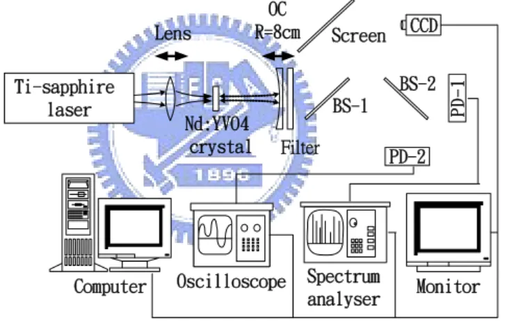
(37) is operated at near-degeneracy, a degenerate resonator is thus a good choice for obtaining laser instabilities.. Previously, we have analyzed an iterative. map of the q-parameter of the resonator [4] and concluded that a laser will become unstable near some degenerate cavity configurations under nonlinear effects.. Using an end-pumped cw Nd:YVO4 laser, we have studied. different laser behaviors under various pump sizes [5,6] when the cavity is near 1/3-transverse degeneracy (g1g2=1/4).. Recently, the Petermann K. factor has also been calculated for maxima on each side of the degeneracy under strong gain guiding or small pump size [7].. It was emphasized that in. the vicinity of the degeneracies the empty-cavity degenerate transverse modes are phase-locked and the resultant radial phase profile depends strongly on the cavity-length detuning.. 3.2 Experiment setup The experimental setup is schematically shown in Fig. 3-1. This laser contains a 1-mm thick Nd:YVO4 laser crystal whose one end face acted as an end mirror and a spherical mirror with radius of curvature of 8 cm as the output coupler (OC). A cw near-TEM00 Ti–sapphire laser at wavelength of 808 nm was used as the pump source, which was focused by a collimating lens onto the crystal so the pump size was adjustable.. The end face of the. crystal, which acted as the end mirror and faced to the pump beam, had a greater than 99.8% reflectivity at 1.064 μm and greater than 99.5% transmission at 808 nm; the other end face comprised an antireflection layer at 1.064 μm to avoid the effect of intracavity etalons. The OC of 10% transmission was mounted upon a translation stage so we could tune the 26.

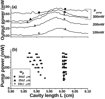
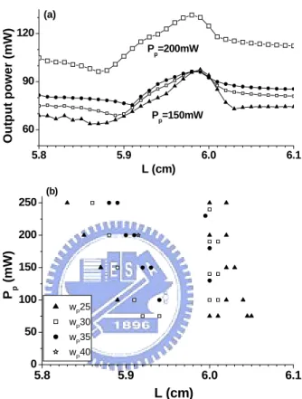
(38) cavity length (L) near the degenerate configuration. The degeneration point of g1g2=1/4, which corresponds to L=6 cm, was determined by the cavity length where the lowest lasing threshold occurs [8]. The laser output was split into two beams, one of which was recorded by a CCD camera and the other was further split into two beams that were individually collected by two photodiodes (PDs) with rise times<0.3 ns.. The signals of the PDs were then. fed into a LECROY-9450A oscilloscope (bandwidth 200 MHz) and an HP8560E RF spectrum analyzer (bandwidth 2.9 GHz), respectively. The Gaussian pump radius, wp, was determined by the standard knife method.. Ti-sapphire laser. Computer. CCD. Screen. BS-2 Nd:YVO4 crystal. BS-1 Filter. Oscilloscope. PD-1. OC R=8cm. Lens. PD-2. Spectrum analyser. Fig. 3-1 The schematic experimental set up. splitter.. Monitor. BS is the beam. 3.3 Experimental results and discussions. 3.3-1 Locations of spontaneous instability. The output power varied with the cavity length under various pump radii and is shown in Fig. 3-2(a). The bottom three curves for wp=19 μm show that a higher pump power not only widens but also heightens the power hump. The laser exhibits a stable cw output for almost entire range of the 27.

(39) studied 3-mm cavity tuning. However, within a narrow range of L on each side of the power hump, denoted as stars in Fig. 3-2(a), we always observed spontaneous instabilities.. The top two curves are the cavity-dependent. output power for wp=25 and 34 μm at a pump power of 300 mW, in which the triangles and the solid circles denote the unstable regions for both cases. Note that the radius of cold-cavity fundamental mode is approximately 108 μm. Summarized in Fig. 3-2(b) are the unstable regions in terms of the. cavity length and the pump power for the three pump sizes of 19, 25, and 34 μm.. We use a single symbol to denote a narrow unstable region while twin. symbols are used to encompass a wider unstable region of about 100 μm. One can see that the unstable regions on the short-cavity side are well separated for different wp and located farther away from degeneracy with increasing the pump power; in contrast, those on the long-cavity side are located very close to the point of degeneration and are nearly independent of the pump power.. 28.

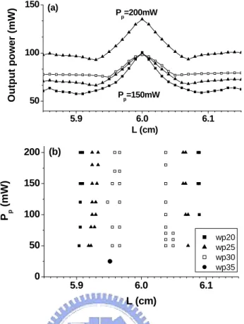
(40) Pump power (mW) Output power (mW). 180. (a). z S. z. 160 S. 140. Ë. 300mW 200mW. Ë. 120. Ppump. Ë Ë. Ë. 100mW. Ë. 100. (b). 300 200 100. Wp z 34±2 μm S 25±2 μm Ë 19±2 μm. 0 5.80. 5.85. 5.90. 5.95. 6.00. 6.05. 6.10. Cavity length L (cm). Fig. 3-2 The observed output power as a function of cavity length (a) and the unstable regions in terms of the cavity length and the pump power for different wp (b). The symbols for wp are the same in (a) and (b). The output power is around 40 mW for Ppump=100 mW as wp=19 μm. Note that we have added 50 mW and 75 mW for the curves of Ppump=200 mW and Ppump=100 mW. The absorption efficiency of Ppump is about 60-70%. The lasing threshold is about 5-30 mW depending on L and wp.. We use our simulation model which was discussed in chapter 2 to simulate the output power with the cavity length and find out the location of instability. Fig. 3-3(a) shows the output power as a function of L!when considering the thermal lens effect. The curves of output power that are labeled as triangles, empty squares, and solid circles for wp=25, 30, and 35 μm, respectively, show asymmetric power humps with respect to the point of. degeneration.. The dependence of the power hump on wp and Pp (the. effective pump power) are the same as in Fig. 3-2(a). The unstable regions are summarized for four values of wp in Fig. 3-3(b), which are similar to those in Fig. 3-2(b) except that the vertical axis of Fig. 3-3 is the effective 29.

(41) pump power that matches with the pump efficiency of ~0.6 taken from the measured pumping. Again, in Fig. 3-3(b) we use a single symbol to denote a narrow unstable region while twin symbols are used to encompass a wider unstable region. It shows similar unstable regions and dependence on wp and Pp as those in Fig. 3-2(b); for example, at wp=35 μm, the unstable region shifts approximately from L=5.94 to 5.90 cm on the short-cavity side as one increases the effective pump power to match with the experimental data in Fig. 3-2(b). Moreover, the far-field intensity profiles beside the long-cavity unstable region are similar to those in Fig. 2(b) of [6].. In addition, no. instability can be observed as wp>40 μm, which is also consistent with the experiment. In order to study the influence of the thermal lens effect, we repeated the simulation without considering the thermal lens effect. The calculated output power and the obtained unstable regions are shown in Fig. 3-4(a) and (b), respectively. As compared with Fig. 3-3, it clearly shows that thermal lens effect leads to certain phenomena: (1) an asymmetrical shape of the power hump; (2) asymmetrical unstable regions with respect to the degeneration point; (3) dependence of the region shift on Pp on the short-cavity side but not on the long-cavity side; and (4) much less shift of the power maximum than shift of the unstable region (e.g., see wp=30 μm and Pp=150 mW). In summary, adding thermal lens effect in simulation model will obtain similar results with the features of instability regions and the diagram of output power versus cavity length in experiment. No matter how the results of experiment or simulation (with thermal lens or without thermal lens effect) 30.

(42) the instability regions are located at the rim of power hump.. If the wp<40. μm, we can easily locate the instability regions by the diagram of output. power versus cavity length.. Output power (mW). (a). 120 Pp=200mW. 90 Pp=150mW. 60 5.8. 5.9. 6.0. 6.1. 6.0. 6.1. L (cm) (b). 250. Pp (mW). 200 150 100 50 0. 5.8. wP25 wP30 wP35 wP40. 5.9. L (cm). Fig. 3-3 The numerical output power as a function of cavity length with considering the thermal lens effect (a) and the unstable regions (b) for different wp. The symbols for wp are the same for (a) and (b).. 31.

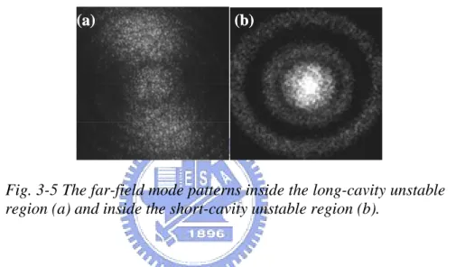
(43) Output power (mW). 150 (a). Pp=200mW. 100. Pp=150mW. 50 5.9. 6.0 L (cm). 6.1. Pp (mW). 200 (b) 150 100 wp20 wp25 wp30 wp35. 50 0. 5.9. 6.0. 6.1. L (cm). Fig. 3-4 The numerical output power as a function of cavity length (a) and the unstable regions (b) without considering the thermal lens effect. The symbols for wp are the same for (a) and (b)/!. 3.3-2 Laser dynamics in instability region. When the cavity length was tuned from the long-cavity side toward and across the point of degeneration, various far-field mode patterns were observed.. The mode pattern shows a near-fundamental Gaussian. distribution far from degeneracy. Tuning L!close to the right edge of the unstable region, we observed a slightly distorted mode pattern. When the cavity was set within about 100 μm of the unstable region, the mode pattern became non-cylindrically symmetric and strongly spread in a special direction as shown in Fig. 3-5(a).. This anomalous spreading pattern. maintained wider than the whole unstable region by few tens of micrometers. When L!was tuned across the range that showed the spreading pattern, the 32.

(44) far-field pattern recovered to a cylindrically symmetric one but turned into many concentric rings with a dark center that is the far-field pattern of the multi-beam-waist mode [6].. By further tuning of L!toward the unstable. region on the short cavity side, we observed the cylindrically symmetric mode pattern as shown in Fig. 3-5(b) that differs from the patterns in the unstable region of the long-cavity side, as indicated in Fig. 3-5(a).. (a). (b). Fig. 3-5 The far-field mode patterns inside the long-cavity unstable region (a) and inside the short-cavity unstable region (b).. We further investigated the temporal behaviors of the output power within the unstable regions at Ppump=260 mW and wp=34 μm. Fig. 3-6(a) shows a periodic time trace when the cavity was tuned at the edge of the long-cavity unstable region. Its corresponding RF spectrum in Fig. 3-6(b) shows one main peak at 1.33 MHz and three harmonics. When the cavity length was decreased by 20 μm from the position of Fig. 3-6(a), a period-2 evolution was observed. The time trace and its spectrum are shown in Fig. 3-6(c) and (d), respectively. On continuing the decreasing of the cavity length, we recorded a chaotic evolution in Fig. 3-6(e) with a broad low frequency spectrum indicated in Fig. 3-6(f). Calculation by use of the chaos data analyzer (American Institute of Physics) shows that the correlation 33.

(45) dimension of the chaotic evolution is approximately 2.1.. Although the. temporal behaviors of the cavity configuration-dependent instabilities are similar on each side of the degeneracy, the high-frequency responses of their power spectra are quite different.. For the long-cavity instabilities we. observed multiple beating frequencies at 812 MHz, 1.63 GHz, and 2.44 GHz (see Fig. 3-6(g)) that were confirmed with a Fabry-Perot interferometer (FPI) having FSR=15 GHz and finesse=150.. The transverse mode beating. pertaining to the Laguerre-Gaussian LG1,0 and/or LG2,0 modes would induce spatiotemporal instability, where the subscripts 1 and 2 are the radial indices and 0 is the azimuthal index. However, within the short-cavity unstable region the spectrum shows only the longitudinal mode beating at 2.44 GHz with the absence of transverse mode beating in both of the RF and the FPI spectra.. 34.

(46) (b). Voltage. Power spectrum (dB). (a). 0. 5. 10. 15. 2f1 3f1. -60. 4f1. -90. 20. 0. (c) Power spectrum (dB). 5. 4. 6. 8. 10. 15. 2. 4. 6. 8. 2. 4. 6. 8. f1 f1/2. -30. -60. -90. 20. 0. (f). Voltage. Power spectrum (dB). (e). 0. 2. (d). Voltage 0. f1. -30. 10. 20. 30. -30. -60. -90 0. 40. Time (μs). Frequency (MHz). Power spectrum (dB). -60 (g) 2.44GHz. -70. 812MHz. 1.63GHz. -80. -90. -100 0.0. 0.5. 1.0. 1.5. 2.0. 2.5. Frequency (GHz). Fig. 3-6 The temporal evolution of laser output. (a) Periodic, (c) period-doubling, and (e) chaotic output within the long-cavity unstable region. The RF spectra (b), (d), and (f), that correspond to (a), (c), and (e), respectively. (g) The high frequency RF spectrum of the spreading mode pattern of Fig. 3-3(a).. To investigate the distinction between the instabilities on the long-cavity 35.

(47) side and those of the short-cavity side, we used two PDs at different transverse positions to simultaneously record the laser power. The first PD was fixed at the center of the profile as the reference and the second one was located at an off-axis position. When the two detectors were separated within a distance, their temporal traces on the oscilloscope were completely the same as shown in Fig. 3-7(a). However, we found for the long-cavity instability that the high peak of one trace coincided with the low peak of the other trace as shown in Fig. 3-7(b) when the two detectors were separated by some specific distance. This reveals that the intensity profile varies with time and thus indicates spatiotemporal instability.. On the other hand,. within the unstable region of the short-cavity, we always observed the same behavior between the two signals no matter at what position the second PD was located. Temporal instability was exhibited on the short-cavity side. In addition, we also found that the instabilities on both sides of the degeneracy are closely related to high-order transverse modes because the instabilities disappeared when a knife-edge was inserted 500 μm into the cavity beam to inhibit the high-order transverse modes. explained in the following paragraph.. 36. This will be.

(48) Voltage. (a). 0. 0. 0. 2. 4. 6. 8. 10. 8. 10. Time (μs). Voltage. (b). 0. 0. 0. 2. 4. 6. Time (μs). Fig. 3-7 The time traces in oscilloscope when the two PDs were separated close to each other (a) and farther away (b) for the long-cavity instabilities.. We will use our simulation model to explain the observations of experiment. To simplify our discussion, we remove the thermal effect in the simulation.. Without the thermal lens effect, not only the power hump. but also the dynamical behaviors are symmetric with respect to the point of 37.

(49) degeneration.. The simulated temporal evolution of the unstable output. power exhibits self-pulsation on both sides of the degeneracy with a pulsing frequency of few hundred kHz (see Fig. 3-8(a)). The simulated intensity profile of each round trip show the variation of the on-axis peak intensity with time as the characteristic feature of Fig. 3-8(a), but the normalized profile varies only a little.. We plotted four normalized intensity profiles in. Fig. 3-11(b) from the pulse peak to valley to show the variation. Their corresponding far-field intensity profiles [insets in Fig. 3-8(b)], having two obvious rings, agree with the photograph of Fig. 3-5(b). Moreover, the far-field intensity profile decreases smoothly and then increases when the pulse is growing.. This leads to pure temporal instability.. The modal. analysis shows that the modes in Fig. 3-8(b) can be decomposed into the combination of the near-degenerate LG0,0, LG3,0, /!/!/, LG18,0 modes with mode weights and relative phase shifts because LG21,0 undergoes large diffraction losses for a 600 μm aperture at the reference plane. These phase shifts must be included because the phase pattern is important as emphasized in [7].. We give a fitted result in the figure caption of Fig. 3-8(b). When. the thermal lens effect is included, the feature of self-pulsation is unchanged for the short-cavity side. This matches with the general expectation that the thermal lens effect will only shift the cavity length.. 38.

(50) (b). Normalized intensity. Output power (arb. units). Intensity (arb. units). 1. (a). 0. 0 4. 0. 4. 2x10. 1x10. 0. 50. 100. 150. 200. (d). 100. 5. 10. 200. 15. 20. 300. 0. Intensity. 0. Intensity (arb. units). (c). Output power (arb.units.). 8. Radial coordinate (μm). Round trips. 0. 4. Angle (mrad). 0. 0. 50. 4 Angle (mrad). 100. 8. 150. 200. Radial coordinate (μm). Round trips. Fig. 3-8 (a) A self-pulsing temporal evolution of the simulated output power without the thermal lens effect for M=5.96 cm. (b) The normalized intensity profiles and their corresponding far-field profiles (inset) from the pulse peak (solid circles) changes to open circles, solid squares and then to the pulse valley (open triangles). The normalized profiles of the open triangles are covered by the solid squares. The modal analysis for the profile of solid squares are LG0,0(0 。 )+0.63 LG3,0(-75 。 )+0.34 LG6,0(-105 。 )+0.16 LG9,0(-90。)+0.08 LG12,0(-83。)+0.08 LG15,0(-116。)+0.07 LG18,0(-93。). (c) The numerical temporal evolution of the output power in the vicinity of the degeneracy with the thermal lens effect for L=6.005 cm. Inset is the first 20 iterations. (d) The intensity profiles and their corresponding far-field profiles (inset) of three successive round trips.. However, on the long-cavity side the region shift seems independent of Pp and the self-pulsation becomes the characteristic feature of Fig. 3-8(c), in which the output power forms three branches of oscillation. The first 20 39.

(51) iterations in the inset show that the output evolution nearly comes back the same value after three round trips; that is the power spectrum indicates one peak at roughly 1/3-longitudinal beating frequency that corresponds to the experimental data of 812 MHz. The intensity profiles of three successive round trips are shown in Fig. 3-8(c), which are not normalized due to the large difference. The corresponding far-field intensity profiles in the inset of Fig. 3-8(d) exhibit a complex feature, which is different from that of the short-cavity side. Unfortunately, we could not yet obtain good fitting data by running the same fitting parameters, even when the LG1,0 mode was included. This may be due to the peculiar phase pattern that is deformed strongly by the thermal lens effect in the vicinity of the degeneracy. Because the beating frequency between the near-degenerate LG modes is absent on both long-cavity and short-cavity instabilities, the frequencies of the near-degenerate LG modes are locked together to a single frequency. Therefore the frequency-locked mode, a supermode [9-10], interacts with the inverted populations and thus leads to the short-cavity instabilities. However, the long-cavity instabilities arise mainly from the frequency beating between the supermode and the other empty-cavity modes. Although the asymmetric (spreading) mode pattern of Fig. 3-5(a) cannot be produced by using the cylindrically symmetric model with single optical frequency, the simulated results agree with the experiment of transverse mode beating. As far as we know, this is the first report that discusses the relationship between the instability and the thermal lens effect. Furthermore, when the aperture on the reference plane is decreased to 450 μm, in accordance with the previous experiment described, the 40.

(52) instability disappears.. The stationary mode now consists of the. near-degenerate LG modes with the same frequency but lack of the higher-order LG15,0 and LG18,0 modes. This fact of transverse mode locking was confirmed by the absence of the near-degenerate mode beating and by the observation of the intensity profile variation with the propagation distance as done in [6].. The supermode lack of the components of the LG15,0. and LG18,0 modes is unable to arise the instability. Inserting a knife-edge into the cavity beam in our experiment also results in a cylindrically symmetric pattern instead of a spreading pattern.. Apparently, the. high-order modes with small amplitude may play important roles in symmetry breaking as indicated in [11].. However, the origin of the. symmetry breaking is still unknown. Going back to Fig. 3-8(a), the pulsation is damped by the relaxation oscillation so the pulsing frequency depends on the pump power and the cavity length. Theoretically, the pulsing spectrum can be calculated from the Fourier transform of the output power evolution. Interestingly, by using γ=105 s which the spontaneous decay rate is scaled 5 times we obtained. periodic pulsing, period-2, and chaotic time evolution of the output power when L!was tuned from 5.96 to 5.951 cm with wp=30 μm and an effective pump power of 100 mW as show in the Fig. 3-9. After 5 times scaling the dynamic behaviors of simulation, which is the route to chaos, are the same as the observations of experiment.. 41.

(53) Output power (arb. units). (a). 0 0. 2000. 4000. 6000. 8000. 10000. 8000. 10000. Round trips. Output power (arb. units). (b). 0. 2000. 4000. 6000. Output power (arb. units). Round trips. (c). 0. 0. 5000. 10000. 15000. 20000. Round trips. Fig. 3-9 The time evolution of self-pulsation by 10 times scaling. (a) periodic, (b) period-doubling, and (c) chaotic output are respectively located at L=5.955cm, 5.9523, and 5.9505cm.. 3.3-3 Cooperative frequency locking and laser patterns. The laser cavity operates at exactly degeneracy, the transverse modes and longitudinal modes will degenerate. It is mean that we can not observe any mode beating on the RF spectrum.. When laser resonator away from the. degeneracy the mode beating should be measured result in none-degenerate 42.

(54) transverse modes. However, we also can not observe any mode beating in our experiment except the instability of long-cavity as section 3.3-2 discussing above.. This phenomenon is called as cooperative frequency. locking [12]. In this section we will use mode expansion to discuss laser patterns around degenerate cavity, and we found that vary large range of cooperative. frequency. locking. where. about. several. millimeters.. Cooperative frequency locking due to their nonlinear coupling several transverse modes lock to a common optical frequency and particular phase differences are selected [13-14].. In the resulting stationary pattern,. amplitudes and relative phases of the interacting modes are determined by the minima of the generalized free energy of the system [15-17]. However, in conventional case, there are only several hundreds micrometer away from degeneracy to maintain frequency locking [18].. 3.3-3.1 Mode expansion and experiment observations. We show the normalized intensity profile and the phase profile on the reference plane with solid circles in Figs. 3-10(a) and (b) at the degeneracy (L = 6 cm) for wp = 30 μm and the effective pump power of 100 mW without considering the thermal lens effect. In order to show the good fitting of mode decomposition using genetic algorithm (GA), we plot the fitted results in Figs. 3-10(a)-(d) with open circles and use the logarithm scale in Fig. 3-10(a).. The mode decomposition is done with 13 fitting parameters. including six amplitude weightings and seven relative phases.. For the. aperture radius of 600 μm on the reference plane, we expand the calculated mode profile into the 1/3-degenerate LGpm modes with p = 0, 3, 6,. . . ,18 and 43.

(55) m = 0, where p!is the radial mode index and m is the angular index. The normalized electric field of LGp0 mode can be expressed as ⎤ ⎫⎪ ⎛ - r 2 ⎞ ⎛ ikr 2 ⎞ ⎧⎪ ⎡ ⎛ z ⎞ ⎟exp⎜⎜ ⎟⎟exp ⎨i ⎢kz - (2p + 1)tan - 1 ⎜⎜ ⎟⎟ + δ p ⎥ ⎬ , E p0 (r, z ) = Ap0 (r, z )exp⎜⎜ 2 ⎟ ⎝ w(z ) ⎠ ⎝ 2R(z ) ⎠ ⎪⎩ ⎣ ⎝ zR ⎠ ⎦ ⎪⎭. (3.1) where wc 0 ⎛ 2r 2 ⎞ ⎟ Ap0 (r, z ) = E0 Lp ⎜ w(z ) ⎜⎝ w(z )2 ⎟⎠. is the modal function, E0 is the normalization constant, zR is the Rayleigh length, w(z) is the beam radius, R(z) is the radius of curvature of the phase front, r and z are, respectively, the radial and axial coordinates, and L0p is the Laguerre polynomial for mode index p.. We assume all the excited LGp0. modes have the same wavenumber and then the intensity profile |η0E00 + η3E30 +… + η18E18,0|2 with seven amplitude weightings η(η0 be fixed unity). and seven relative phases δp is fitted to the mode-calculation profile. We see that the resultant fitted profiles match with the mode-calculation profiles extremely well in Figs. 3-10(a)-(d). From Fig. 3-10(a) the central lobe of the intensity profile is near-Gaussian with the waist radius of ~30 μm (approximately equals to the pump radius, see the solid curve in the inset with linear scale), which shows that the laser is strongly gain-guided. Note that the radius of the fundamental mode, w0, is 108 μm. The seriously saturated gain distribution is shown with the dashed curve in the inset of Fig. 3-10(a). The gain distribution is obtained from the term exp(σΔOd) in Eq. (2.11), where ΔO!is r-dependent. Fig. 3-10(b) shows that the phase profile is flat within r!= 200 μm but discontinuously jumps π phase at some positions 44.