在無線網路中為大的I型式畫面所設計之具有型式判別能力的錯誤控制

國 立 交 通 大 學

電信工程學系碩士班

碩 士 論 文

在無線網路中為大的 I 型式畫面所設計

之具有型式判別能力的錯誤控制

Type Aware Error Control for Large I-Frames

in Wireless Networks

研究生: 廖根良

指導教授:廖維國 博士

在無線網路中為大的 I 型式畫面所設計

之具有型式判別能力的錯誤控制

Type Aware Error Control for Large I Frames

in Wireless Networks

研究生: 廖根良

Student:

Liao,

Gen-Liang

指導教授: 廖維國 博士

Advisor:

Dr.

Liao,

Wei-Kuo

國 立 交 通 大 學

電信工程學系碩士班

碩士論文

A Thesis Submitted to

the Department of Communication Engineering

College of Electrical Engineering and Computer Science

National Chiao Tung University

in Partial Fulfillment of the Requirements

for the Degree of Master of Science

In

Communication Engineering

Aug 2008

在無線網路中為大的 I 型式畫面所設計

之具有型式判別能力的錯誤控制

研究生: 廖根良

指導教授: 廖維國 博士

國立交通大學電信工程學系碩士班

中文摘要

針對互動式影像服務我們提出了要傳送不同大小影像畫面的錯誤控制. 錯 誤控制的行為例如重傳和增加冗餘碼都被考慮. 為了得到低延遲和小延遲差距, 我們選用的SFQ排程器是一個適合處理具有變動位元流量的影像應付的排程器. 當嚴密的檢查問題, 我們發現大的I型畫面, RS碼以及影像畫面之間短暫的相互 關連性這些要素深深地影響畫面失去率,有效率地處理它們是非常的具挑戰性的. 在這篇論文裡, 我們延續了之前針對固定大小畫面, 基於馬可夫的錯誤控制的 成果來做. 在我們的模擬裡, 在寬頻考量下, 將通道特徵化成兩個狀態的模型, 且狀態的停留時間是根據二階Erlang分佈. 我們的數值模擬展示了我們提出的 方法在所有模擬設定降低了失去畫面的比率. 除此之外, 我們的數值模擬有效 的降低了重傳次數和使得碼率多元化.

Type Aware Error Control for Large I

Frames in Wireless Networks

tract

Student: Liao, Gen-Liang Advisor: Dr. Liao, Wei-Kuo

Department of Communication Engineering

National Chiao Tung University

Abstract

We propose an error control for delivering video frames of different sizes for interactive video service. The error control actions such as retransmission and adding redundancy codes are considered. For the purpose of low delay and small jitter, we use start-time fair queuing which is a suitable scheduling algorithm for video

applications that have variable bit rate. When examining closely, we find that factors of the large I-frame, redundancies of RS-code, the temporal correlation between video frames significantly impacts the frame loss rate but dealing with them effectively is very challenging. In this thesis, we extend the early work of MDP-based error control for fixed size frames to do so. In our simulation, characterizing the channel by a two-state model where state durations follow the Erlang distribution of second order under wideband is considered. Our simulation shows that our proposed method reduces frame loss rate in all the simulation settings. Besides, it effectively reduces retransmission times and makes code-rate diversity.

誌謝

首先, 謝謝老師這兩年來的指導. 在做助教的過程中, 學到了許

多網路以及程式語言的概念. 行為以及學習模式上,也學到如何對自

己進行有效率的訓練. 並感謝口試委員委-張文鐘老師, 黃家齊老師

的指導

再來, 謝謝實驗室的學長姐,同學. 碩零時, 裕祥和為凡給予我

實驗室器材維修的技巧, 碩二上時, 賢宗指導我 UML 的概念受益良

多. 永裕, 柯柯, 俊宏, 郁媛, 宇哲,國瑋, 在這兩年的相處讓我學

習到不少與人類的互動, 特別感謝宇哲在碩一下系電的果斷, 讓我

課業壓力減輕許多, 真是謝謝.

謝謝女朋友-王曼卉. 全省最強的她, 五年多來的陪伴, 陪我度

過無數的谷底,挫折, 以及一起增加人生經驗.我們的花栗鼠-小泡芙,

四年多的相處, 排解了我的煩悶.

最後, 感謝我老爸老媽三姐四姐, 沒他們對我的信任支持和維持

家計, 我沒辦法和小曼在新竹完成學業. 謝謝.

Contents

Chinese Abstract……….……….…………..………….……Ⅲ English Abstract……….……….……….…………..…Ⅳ Acknowledgment……….……….……….………….…Ⅴ Contents……….……….………Ⅵ List of Tables……….………….………..…..Ⅶ List of Figures……….………….……….….……Ⅶ Introduction……….……….………..……..1 Background Knowledge……….…….………...4 2.1 video-hierchy……….…….………...4 2.2 RS code…..……….…….……….….……….…...…6

2.3 Start-time fair queuing………...6

2.4 Markov Decision Process………..……….…………...7

1. Policy iteration method……….….………9

2. The value-determination operation……….….…………...……...…9

3. The policy-improvement routine……….…….……….…..10

System and Model……….….…………..………..13

3.1 Input-Trace………..……….….……….………13

3.2 system………..….………….….……14

1. Hybrid ARQ and FEC……….….………...….…15

2. Transmitter……….……….….………15

3. Receive……….………..………...16

3.3 Channel Model……….………..………...16

Problem Formulation Based on MDP……….……….……….…...18

4.1 State Definition……….……….…....18 4.2. Policy Definition……….………...……….19 4.3. Cost-Function……….………...19 4.4. State-Transition-Probability.………...…..…….………20 4.5. Policy Iteration……….………...21 Simulation Design……….……….……….22 5.1. OMD Design...22 5.2. Scenario Design………..….……….………24 1. Case 1……….….….…….……...24 2. Case 2...…...25 Simulation Result………...26 Conclusion………..… 35 Reference……… 36

List of Tables

Table 4-1 Total Policy……….……….19

Table 6-1 figure 6-1 in details……….……….30

Table 6-2 figure 6-2 in details……….……….30

Table 6-3 early drop, normal case in details………31

Table 6-4 early drop, premium case in details……….31

Table 6-5 no early drop, normal case in details………..….………32

Table 6-6 no early drop, premium case in details……..….……….32

Table 6-7 hybrid ARQ code-rate = 0.9, normal case….…..………33

Table 6-8 hybrid ARQ code-rate = 0.9, premium case………33

Table 6-9 hybrid ARQ code-rate = 0.8, normal case...………34

Table 6-10 hybrid ARQ code-rate = 0.8, premium case………..…34

List of Figures

Figure 2-1 typical composition of a video sequence…...5

Figure 2-2 The Policy-Iteration cycle………..11

Figure 3-0-0 Input-Trace………..…...13

Figure 3-0-1 Input-Trace……….14

Figure 3-1 System frame work………....14

Figure 3-2 Channel Model………...16

Figure 4-1 Transition Probability……….………20

Figure 5-1 OMD…...22

Figure 5-2 Scenario 1...24

Figure 5-3 Scenario 2……….………..25

Figure 6-1 FLR-BER premium case……….………...27

Figure 6-2 FLR-BER normal case……….………..27

Figure 6-3 Hybrid ARQ with code-rate 0.8 and 0.9 code-rate utility….……….28

Figure 6-4 Early Drop and No Early Drop code-rate utility………….………...29

Abbreviation

Group of picture GOP

Markov Decision Problem MDP

Luminance Y

Hue U

Intensity V

Chapter 1

Introduction

Nowadays, efficient video-transport over wireless networks is demanding when requirements of multimedia communication grow up explosively. The issue of packet loss in wired networks has been extensively studied. However, unlike wired networks, packet delivery in wireless network suffers time-varying and bursty errors due to the effects such as near-far effect and multi-path fading. Worse yet, in dealing with the streaming video transmission, more packet loss could be experienced due to the temporal correlation of frames in one group of picture (GOP), i.e., a loss of a

reference frame implies the loss of all those frames which need the reference frame to decode.

In [1] and [2], an error control mechanism using a hybrid ARQ control mechanism by estimating channel condition is proposed. Briefly put, their error control is letting the MAC layer at transmitter choose a proper code-rate according to the feedback information. Nevertheless, the information from feedback is not enough for video-transmission when deciding code-rates. For example, a last frame of one GOPwhich decided lower code-rate results in the subsequent I-frame over-flow when buffer is full. Consequently, we enhance information accuracy by characterizing connection with four parameters in order to decide the most proper code-rate by

Markov Decision Problem (MDP).

In this thesis, we consider devising error control for delivering video frames of different sizes for interactive video services. When examining the problem more closely, we find the effect of large I-frame along with redundancies of RS-code is most difficult to deal with. Because I frame results from exploiting spatial

redundancies, it is large than the others which arises from exploiting temporal

redundancies from this I frame in the same GOP. Such Variable bit rate should not be penalized in future for using extra bandwidth available now. Besides, due to

multiplexing, we need to ensure the bandwidth minimum for each flow to reach low delay and little jitter. Consequently, we use start-time fair queuing for video-transport that has variable bit rate to deal with the above-mentioned considerations.Therefore, the large I frame implies lengthy inter-polling time and thus results longer delay to transmit the following frames in the same connection. As a result, the following frames will be obsolete because the deadline is missed.

scheduling algorithm in order to deal with video-traffic-burstiness. However, their emphasis is on exploring the multi-user diversity gain. For code-rate efficiency, frame loss seems to be inevitable. In [4] and [5], they use selectively frame discard to minimize the effect of their loss on the QoS but they consider large buffer and do not mention a hybrid ARQ control mechanism. In [9], a MDP-based error control has been proposed. A MDP-based error control is a hybrid error control by receiving returning information from flows and channel. Code-rates and the number of dropping packets in the buffer are decided by MDP in light of returning information. A proper code-rate can reduce retransmission times and a proper number of dropping packet in the buffer which we called early-drop makes code-rates diversity. They exploit MDP to find these proper decisions.

In video transmission, we observe that the first frame in one GOP which we call I frame is more than three times as large as the other frames in the same GOP from figure 3-0-1. It hints that the same buffer suffers a lot of arrival packets in the next time if I-frame transmits now. This phenomenon almost results in overflow. Video transmission hints that a large inter-polling and variable packet size in one GOP. It is totally different to [9]. They only consider fixed packet size and it may cause many frame loss because of no consideration about large I frames. As a result, we mainly extend [9] by handling the phenomenon which I frame causes.

In the past, the channel is characterized by a two-state Markov chain, which is widely accepted to model the Rayleigh fading channel. However, as the channel becomes frequency-selectively channel under wide-band, from [6], the two-state Markov chain is no longer suitable to characterize the channel. As a result, we refer to [6] and characterize channel as the two-state model where state durations follow the Erlang distribution of second order, rather than the exponential distribution. By [6, Table-2]: % of frames in error from the simulator and from the experimental data is similar.

Our simulation shows that a MDP-based error control for large I frames reduce frame loss rate. Furthermore, it effectively reduces retransmission times and makes code-rate diversity.

The rest of the thesis is organized as follows: In the chapter 2, we describe the necessary background knowledge about policy iteration method of Markov Decision Process for simulation, Reed–Solomon (RS) code, start time fair queuing, and video-hierarchy. In the chapter 3, we discuss the scope of this problem and give overview to our system architecture. In the chapter 4, we formulate the problem to Markov Decision Process, and find out the best policy by using the policy iteration method mentioned in the chapter 2. In the chapter 5, we introduce

In the chapter 6, we show the simulation result to demonstrate that our method is better than the others. In the chapter 7, we make a conclusion.

Chapter 2

Background knowledge

In this chapter we will introduce the basic concept of video hierarchy [8], RS-code [2], start-time fair queuing [7] and Markov Decision Process [11] with rewards and give formal definition to reward, alternative, expected cost value, and policy. We also introduce the Policy iteration method, which will lead us to find the optimal policy for the system.

2.1 Video Hierarchy

It is an introduction to digital video. We will introduce pixel, YUV, sub-sampling, video hierarchy, and video compression to explain the reason why video transport needs video-compression.

The common color space in the computer domain is based on the three component colors red, green, and blue. A pixel can be defined by these three components and usually added a component alpha to represent 32 bits full color in the computer.

In order to easily adjust TV signal for users, the pixels are transformed to three different components the luminance component (Y), and the two chrominance

components hue (U) and intensity (V) when video transport. The conversion between theses two color spaces is defined a fixed matrix. The following is 8 bit digital environments from [8].

For PAL systems,

⎥ ⎥ ⎥ ⎦ ⎤ ⎢ ⎢ ⎢ ⎣ ⎡ ⎥ ⎥ ⎥ ⎦ ⎤ ⎢ ⎢ ⎢ ⎣ ⎡ − − − − = ⎥ ⎥ ⎥ ⎦ ⎤ ⎢ ⎢ ⎢ ⎣ ⎡ B G R V U Y ‧ 100 . 0 515 . 0 615 . 0 436 . 0 289 . 0 147 . 0 114 . 0 587 . 0 299 . 0 For NTSC systems, ⎥ ⎥ ⎥ ⎦ ⎤ ⎢ ⎢ ⎢ ⎣ ⎡ ⎥ ⎥ ⎥ ⎦ ⎤ ⎢ ⎢ ⎢ ⎣ ⎡ − − − − = ⎥ ⎥ ⎥ ⎦ ⎤ ⎢ ⎢ ⎢ ⎣ ⎡ B G R Q I Y ‧ 31135 . 0 522591 . 0 211456 . 0 321263 . 0 274453 . 0 595716 . 0 114 . 0 587 . 0 299 . 0

The Y, U, and V values can be stored for each individual pixel and this format is referred to as YUV 4:4:4. However, the human eye is more sensitive to changes in luminance than to the other components. For this reason, it is common to reduce the information that is stored per picture by chrominance sub–sampling.With

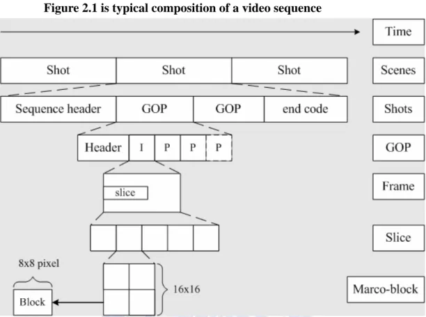
Figure 2.1 is typical composition of a video sequence

A video sequence consists of many scenes, and a scene consists of many shots. For example, scene-A is a dinner party scene and scene-B is sleep scene after the dinner party. The numbers of shot that a scene has is the numbers of camera in this scene. Nevertheless, we emphasize that the video-trace in our experiment is only one scene and one camera. Therefore, the video-sequence hints many GOPs in our experimental video-trace. Another important observation is that the levels that are most relevant for video encoding and decoding are from the GOP level downwards. The sub-sampling is been used at block level, and YUV 4:2:0 is been used usually.

Based on the above reasons, we concentrate on video-compression about our video-trace. Video compression exploits two types of redundancies in our

experimental video-trace：

1. Intra-frame encoding ( spatial redundancy )：On a per–frame basis, neighboring pixels tend to be correlated and thus have spatial redundancy. Intra-frame encoding is employed to reduce the spatial redundancy in a given frame.

2. inter-frame coding ( temporal redundancies )： Consecutive frames have similarities and therefore temporal redundancy. These temporal redundancies are reduced by inter-frame coding techniques.

To sum up section 2.1, video transport needs video-compression to reduce bandwidth requirement. However, highly VBR and long rang dependency caused by video-coding needs to be overcome.

2.2 Reed-Solomon (RS) Codes

For the error control of user data, we adopt RS codes over in which the codeword size

) , ,

(N K q GF(q)

N and the number of information symbols . A -ary symbol is mapped to bits, so . RS codes are known to have the maximum error -correction capability for given redundancy, i.e., a maximum distance separable (MDS) code. ) N ( K < q b q=2b

For an MDS code, the minimum distance is determined as , where the error correction capability

) , (N K 1 + min d min min = N −K d t=(d −1)/2=(N −k)/2,

i.e., any combination of symbol errors out of t N symbols can be corrected. The

code rate rc is defined as rc =K/N. One can easily see that the more parity

symbols (i.e., larger N − ), the better error-correction capability. RS codes are K

also known to be efficient for handling burst errors. For example, with RS code with the error correction capability , as many as

) 2 , , (N K b t b t⋅ bit errors can be corrected in the best case when all of bits in each of -bit symbols are erroneous (i.e., burst errors). But only bit errors can be corrected in the worst case when only one bit in each of -bit symbols is erroneous (i.e., non-burst errors).

b

t

tb

tb

Originally, the codeword size of RS code is determined to be . However, a shorter codeword can be obtained via code shortening. For example,

given a code, ) , , (N K q q−1 ) , ,

(N K q K − information symbols are appended by zero s

symbols. These

s

K symbols are then encoded to make an N symbol-long codeword.

By deleting all zero symbols from the codeword, we can obtain code. For decoding this shortened code, the original decoder can still be used by appending zero symbols between

s (N −s,K −s)

) , (N K s

K− information symbols and N − parity K

symbols. Shortened RS codes are also MDS codes. Code shortening is useful especially for transmitting information with less than K symbols.

2.3 Start-time Fair Queuing

Video applications have variable bit rate, it should not be penalized in future for using extra bandwidth available now. Scheduling algorithm should ensure fairness even when available bandwidth varies.

In Start-time Fair Queuing (SFQ) algorithm, two tags, a start tag and a finish tag, are associated with each packet. However, unlike WFQ and SCFQ, packets are scheduled in the increasing order of the start tags of the packets. Furthermore, is defined as the start tag of the packet in service at time t. The complete algorithm is

( )

defined as follows:

1. On arrival, a packet p_fj is stamped with start tag S p( _fj), computed as:

1

( _fj) max{ ( ( _fj)), ( _fj )} 1,

S p = v A p F p − j≥ (2.1) where F p( _fj), the finish tag of packet p_fj, is defined as:

( ) ( ) 1 j f j j f f f l F p S p j r = + ≥ , (2.2) where F p( 0_f)=0 and r_f is the weight of flow f

2. Initially, the server virtual time is 0. During a busy period, the server virtual time at time t , ( )v t , is defined to be equal to the start tag of the packet in service at time t . At the end of a busy period, ( )v t is set to the maximum of finish tag assigned to any packets that have been serviced by time t .

3. Packets are serviced in increasing order of the start tags; ties are broken arbitrarily.

2.4 Markov Decision Process

Suppose that an N-state Markov process earns rij dollars when it makes a

transition from state i to state j. We call rij the “reward” associated with the transition

from i to j. the set of rewards for the process may be described by a reward matrix R with elements rij. The rewards need not be in dollars, they could be voltage levels,

units of production, or any other physical quantity relevant to the problem.

The Markov process now generates a sequence of rewards as it makes transitions from state to state. The reward is thus a random variable with a probability

distribution governed by the probabilistic relations of the Markov process. One question we might ask concerning is: What will be the player’s expected winning in the next n transitions if the process is now in state i? To answer this question, let us define vi (n) as the expected total rewards in the next n transitions if

the system is now in state i. Some reflection on this definition allows us to write the recurrent relation,

1 ( ) [ ( 1)] 1, 2, , 1, 2, 3, , N i ij ij j j v n p r v n i N n = =

∑

+ − = _L = _{L (2.3)} Where the pij is the transition probability of state i to state j. If the system makes a

transition from i to j, it will earn the reward rij plus the amount it expects to earn if it

starts in state j with one move fewer remaining. As shown in Eq. 2.3, these rewards from a transition to j must be weighted by the probability of such a transition, pij, to

obtain the total expected rewards. Notice that Eq. 2.3 may be written in the form

1 1 ( ) ( 1) 1, 2, , 1, 2, 3, , N N i ij ij ij j j j v n p r p v n i N n = = =

∑

+

∑

− = _L = _L (2.4) If a quantity q_i is defined by (2.5) 1

1, 2,

, .

N i ij ij j

q

p r

i

=

=

∑

=

_{L N}

L Takes the form

1 ( ) ( 1) 1, 2, , 1, 2, 3, . N i i ij j j v n q P v n i N n = = +

∑

− = _L = (2.6)

The quantity qi may be interpreted as the reward to be expected in the next

transition out of state i; it will be called the expected immediate reward for state i. Rewriting Eq. (2.3) as Eq. (2.6) shows us that it is not necessary to specify both a P matrix and an R matrix in order to determine the expected earnings of the system. All that is needed is a P matrix and a q column vector with N components qi. The

reduction in data storage is significant when large problems are to be solved on a digital computer. In vector form, Eq. (2.6) may be written as

(2.7)

( )

n

= +

(

n

−

1)

n

=

1, 2, 3,

,

v

q

Pv

L

Where is a column vector with N components , called the total-value vector.

) (n

v vi(n)

Consider a completely ergodic N-state Markov process described by a transition-probability matrix P and a reward matrix R. Suppose that the process is allowed to make transitions for a very, very long time and that we are interested in the earnings of the process. The total expected earnings depend upon the total number of transitions that the system undergoes, so that this quantity grows without limit as the number of transitions increases. A more useful quantity is the average warnings of the process per unit time. This quantity is meaningful if the process is allowed to make many transitions; it was called the gain of the process.

Since the system is completely ergodic, the limiting state probabilitiesπi are

independent of the starting state, and the gain g of the system is

1 , N i i i g πq = =

∑

(2.8) where qi is the expected immediate return state i defined by Eq. (2.5).

I. The policy-Iteration Method

The policy-iteration method that will be described will find the optimal policy in a small number of iterations. It is composed of two parts, the value-determination operation and the policy-improvement routine. We shall first discuss the

value-determination operation.

II. The Value-Determination Operation

Suppose that we are operating the system under a given policy so that we have specified a given Markov process with rewards. If this process were to be allowed to operate for n stages or transitions, we could define vi (n) as the total expected reward

that the system will earn in n moves if it starts from state i under the given policy. The quantity vi (n) must obey the recurrence relation Eq. (2.7). There is no need

for a superscript k to appear in this equation because the establishment of a policy has defined the probability and reward matrices that describe the system. For completely ergodic Markov processes vi (n) had the asymptotic form:

( )

i = 1, 2, ... , N for large n.

i i

v n

=

ng

+

v

(2.9) We are then justified in using Eq. (2.9) in Eq. (2.6). We obtain the equations

1 1 1 1 1 [( 1) ] i = 1, 2, ... , N ( 1)

Since 1, these equations become

1, 2,..., N i i ij j j N N i i ij ij j j j N ij j N i i ij j j ng v q p n g v ng v q n g p p v p g v q p v i N = = = = = + = + − + + = + − + = + = + =

∑

∑

∑

∑

∑

(2.10)

We have now obtained a set of N linear simultaneous equations that relate the quantities vi and g to the probability and reward structure of the process. However,

account of unknowns reveals N vi and 1 g to be determined, a total of (N+1)

adding a constant a to all vi in Eqs. (2.9). these equations become 1 ( N i i ij j j g v a q p v a = + + = +

∑

+ ), _j n

),

j Or 1 . N i i ij j g v q p v = + = +

∑

The original equations have been obtained once more, so that the absolute value of the vi cannot be determined by the equations. However, if we set one of the vi equal

to zero, perhaps vN, then only N unknowns are present, and the Eq. (2.8) may be

solved for g and the remaining vi. Notice that the vi so obtained will not be those

defined by Eq. (2.7) but will differ from them by a constant amount. The vi produced

by the solution of Eq. (2.8) with vN = 0 will be sufficient for our purposes; they will be

called the relative values of the policy.

We have now shown that for a given policy we can find the gain and relative values of that policy by solving the N linear simultaneous equations with vN = 0. We

shall now show how the relative values may be used to find a policy that has higher gain than the original policy.

III. The Policy-Improvement Routine

We found that if we had a optimal policy up to stage n, we could find the best alternative in the ith state at stage n+1 by maximizing

1 ( ), N k k i ij j j q p v = +

∑

(2.11) over all alternatives in the ith state. For large n, we could substitute Eq. (2.9) to obtain

1

(

N k k i ij j

q

p ng

v

=

+

∑

+

(2.12) as the test quantity to be maximized in each state. Since

1 1, N k ij j p = =

∑

the contribution of

ng and any additive constant in the vj becomes a test-quantity component that is

independent of k. Thus, when we are making our decision in state i, we can maximize (2.13) 1

,

N k k i ij j

q

p

=

+

∑

v

_j

with respect to the alternatives in the ith state. Furthermore, we can use the relative values (as given by Eqs. (2.9)) for the policy that was used up to stage n.

The policy-improvement routine may be summarized as follows: For each state i, find the alternatives k that maximizes the test quantity using the relative values determined under the old policy. The alternative k now becomes di, the

decision in the ith state. A new policy has been determined when this procedure has been performed for every state.

1 , N k k i ij j q p = +

∑

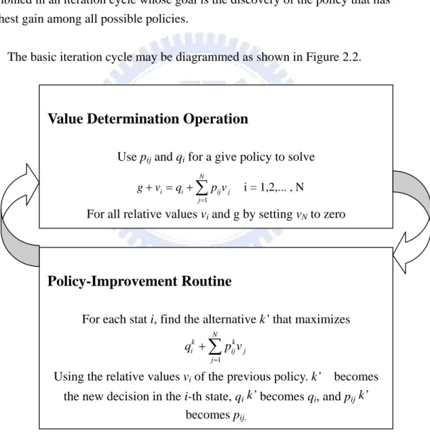
v_j

We have now, by somewhat heuristic means, described a method for finding a policy that is an improvement over our original policy. We shall soon prove that the new policy will have a higher gain that the old policy. First, however, we shall show how the value-determination operation and the policy-improvement routine are combined in an iteration cycle whose goal is the discovery of the policy that has highest gain among all possible policies.

The basic iteration cycle may be diagrammed as shown in Figure 2.2.

Value Determination Operation

Use pij and qi for a give policy to solve

1 i = 1,2,... , N N i i ij j j g v q p v = + = +

∑

For all relative values vi and g by setting vN to zero

Figure 2-2 The iteration cycle.

Policy-Improvement Routine

For each stat i, find the alternative k’ that maximizes

1 N k k i i j q p = +

∑

_jv_j

Using the relative values vi of the previous policy. k’ becomes

the new decision in the i-th state, qi k’ becomes qi, and pij k’

The upper box, the value-determination operation, yields the g and vi

corresponding to a given choice of qi and pij. The lower box yields the pij and qi that

increase the gain for a given set of vi. In other words, the value-determination

operation yields values as a function of policy, whereas the policy-improvement routine yields the policy as a function of the values.

We may enter the iteration cycle in either box. If the value-determination operation is chosen as the entrance point, an initial policy must be selected. If the cycle is to start in the policy-improvement routine, then a starting set of values is necessary. If there is no a priori reason for selecting a particular initial policy or for choosing a certain starting set of values, then it is often convenient to start the process in the policy-improvement routine with all vi = 0. In this case, the

policy-improvement routine will select a policy as follows: For each i, it will find the alternative k’ that maximizes qik and then set di = k’.

This starting procedure will consequently cause the policy-improvement routine to select as an initial policy the one that maximizes the expected immediate reward in each state. The iteration will then proceed to the value-determination operation with this policy, and the iteration cycle will begin. The selection of an initial policy that maximizes expected immediate reward is quite satisfactory in the majority of cases.

At this point it would be wise to say a few words about how to stop the iteration cycle once it has done its job. The rule is quite simple: The final robust policy has been reached (g is maximized) when the policies on two successive iterations are identical. In order to prevent the policy-improvement routine from quibbling over equally good alternatives in a particular state, it is only necessary to require that the old di be left unchanged if the test quantity for that di is as large as that of any other

alternative in the new policy determination.

In summary, the policy-iteration method described has the following properties: z The solution of the sequential decision process is reduced to solving sets of

linear simultaneous equations and subsequent comparisons.

z Each succeeding policy found in the iteration cycle has a higher gain than the previous one.

z The iteration cycle will terminate on the policy that has largest gain attainable within the realm of the problem; it will usually find this policy in a small number of iterations.

Chapter 3

System and Model

In this chapter, we will show the architecture of the system and the channel model which we consider about. There are two major parts in our architecture of system. We separate this chapter into three sections to make framework obvious.

3.1 Input-Trace

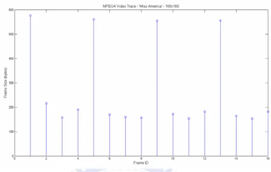
Figure 3-0-0

We use MPEG-4 trace consists of 19196 frames. One frame equals one packet. The detail about our video-trace is as follows：

1. Consist of only I and P frames in order – I, P1, P2, P3 2. I frames are coded autonomously

3. P frames are coded in reference to the most recent I or P frame. 4. The video frames are ordered in the strictly increasing frame number. 5. If an I-frame loss means the whole GOP is loss.

Figure3-0-1

Figure 3-0-1 is video-sequence in details from frame 0 to frame 15. The ratios of I to P is 3.24. We concentrate on large I frame and notice that too long inter-polling time causes video-traffic-burstiness. Real-time data in FIFO queue will be pushed when buffer over-flow and possibly caused a series of drop

In order to deal with such situation, we both have considered this case in MDP in advance and use SFQ as our scheduler.

3.2 System

I.

Hybrid FEC and ARQ ：

We adopt a hybrid of FEC and ARQ, i.e., when errors are successfully corrected, an acknowledgment (ACK) is transmitted to the sender. On the other hand, a negative acknowledgment (NAK) is sent when errors are detected but not correctable. When the sender receives NAK, the packet will keep in the buffer and the packet is waiting to be sent again, and when it receives ACK, it is ready to send the next packet.

A combination of ARQ and FEC is used to improve the QoS performance in the wireless network. Several hybrid ARQ/FEC mechanisms have been proposed in the wireless literature, in our study, we consider a particular combination in which cyclic redundancy check (CRC) is first applied to a packet, followed by FEC. We assume a very strong CRC code, with 100% error detection capability.

Note that the purpose of FEC here is to reduce the number of retransmissions. However, too low code-rate probably accompanies too much redundancy, it cause video-traffic-burstiness. As a result, we should seek a group of code-rate for suiting video-transport.

II. Transmitter：

There are N identical flows in transmitter. Each of them has the same traffic stream and one finite and little buffer. It hints I-frame may appear in the head of line at the same time. The buffer has capacity of M packets. Based on the start-time fair queuing algorithm, the scheduler decides which flow can use the connection. When the buffer is full, new arrival packet will push out the head-of-line packet. Here, we suggest that the packet is pushed because of exceeding its deadline.

In order to resist the getting deteriorated channel, we decide to transmit packet with lower code-rate. Once again, the lower code rate we use, the more redundancies we have to transmit. By start-time fair queuing algorithm, we observe that we will waste bandwidth for transmitting too many redundancies and that will cause the transmitter to push the head-of-line packet. It is a tradeoff, and we focus on tuning the group of code-rate to minimize the cost.

We emphasis that we need to avoid video-traffic-burstiness caused by large I frame and too many redundancies when use RS-code. For a MPEG file, there are relative importances of frame. In order to utility code-rate efficiency for reducing the retransmission times and take frame priority into consideration, frame-loss is

their loss on the QoS. From the view of these, we take little and limited buffer into consideration and exploit MDP to control SFD. When channel getting deteriorated or the bandwidth is little, we may need to drop the less important packets and transmit the important packets.

Finally, the detail of a frame which be transmitted is that frame is applied to RS-code directly. We ignore IP-header and MAC-header because that the inaccuracy is less than 1%.

III. Receiver：

At the receiver side, an arriving packet is passed through a FEC decoder followed by a CRC decoder. If the packet is error, then a negative acknowledgement (NAK) is send back to the sender. The sender needs to retransmit the error packet if the packet still reserve in the buffer.

3.3 Channel Model

Figure 3-2

The channel is characterized by a two-state Markov chain, which is widely accepted to model the multi-path fading channel. Under wideband circumstance, the channel becomes frequency-selective-channel. From [6], we characterize channel as the two-state Markov chain model that its state durations follow the Erlang

distribution of second order. By [6]-TableⅡ：% of frames in error from the simulator and from the experimental data is similar.

The t0, 1, t1, 0, t0, 0, and t1, 1 are transition probabilities in figure 3-2, and they can

be transformed to state duration equivalently. Assuming that packet errors during a given channel state are independent, the probability that a received packet contains a

non-correctable when the channel is in the Good state is given by [2]： b g b g s i N g s i g s N t i g T

P

P

P

P

i

N

P

)

1

(

1

)

1

(

*

*

, , , , 1 ,

−

−

=

−

⎟⎟

⎠

⎞

⎜⎜

⎝

⎛

≤

− + =

∑

where

P

s, g is symbol error when the channel is in the Good state, and

P

b, g is bit error

when the channel is in good state. Similarly,

P

s, b is symbol error when the channel is

Chapter 4

Problem Formulation Based on MDP

In this chapter, we will formulate our problem to Markov Decision Process by introducing components of state, components of policy, cost function, and state transition probability in order.

After we realize these elements, we will find the best policy by using the policy iteration method mentioned in the chapter 2. The maximum gain we have, the minimum cost on frame-loss when video transports we have.

4.1 State Definition

There are 64 states in ours Markov-chain. Each state consists of four parameters： 1. Channel state：The basic concept of hybrid ARQ is from [2].

Naturally, we apply RS-code when the channel gets deteriorated, and apply ARQ when the channel is in lower BER. Consequently, we define the channel

parameter.

2. Loss window：We assume that packet-loss is caused by either dropping packet or pushing packet if the transmitter sends packet to receiver successfully, window will set to zero. Furthermore, video-transport needs video-compression but it results in dependency-drop possibly. Combination of these considerations, we assume that the maximum value of window is 1 to reveal such information about loss duration.

3. Color：Because of intra-frame-coding and inter-frame-coding, frames have priority. From the view of frame priority, we define color parameter to provide help to drop less important frame.

4. Number of packet in the buffer：From the view of the practical implement, the buffer is little and small. In order to resist video-traffic burstiness, we consider the number of packet in the buffer to help drop less important frame when buffer tends full.

4.2 Policy Definition

We have twelve actions in our action space. Each action is a combination of different code rate and different numbers of dropping packets. The possible policies are illustrated in Table 4-1.

Table 4-1

Drop Code-Rate Policy no. 0 1 0 0 0.9 1 0 0.8 2 1 1 3 1 0.9 4 1 0.8 5 2 1 6 2 0.9 7 2 0.8 8 3 1 9 3 0.9 10 3 0.8 11

There are 12 policies in ours Markov-chain. Each policy consists of two parameters：

1. RS code-rate：the options are 1, or 0.9, or 0.8. We are aware of too lower code-rate caused too long inter-polling-time though it has good correct capability. Such situation possibly results in a series of dependency-drop. From [10]-Fig4, we choose these code-rates.

2. the number of dropping packet：the options are 0, or 1, or 2, or 3. They take dependency-drop and early-drop into consideration. For example, buffer arranges P1, P2, and P3 in order but the I-frame is loss. It results in drop the all packets in the buffer.

We expect that the utilities of code-rate are diversity. It hints effective FEC and effectively reduces retransmission times

4.3 Cost-Function

4.4 State Transition Probability

The state transition diagram of the Markov chain Pi, j (k) and

C

i, j (k)

represent the transition probability and cost from state i to state j with policy k in the figure 4.1

Figure 4-1

In order to obtain

P

ij (k)

, we have to denote some notations：

1.

t

0,0denote the transition probability from good state to good state, and

t

0,1

denote the transition probability from good state to bad state, and

t

1,0denote the

transition probability from bad state to good state, and

t

1,1 denote the transition

probability from bad state to bad state

2. The probability

P

T, g is packet error probability in good state,

P

T, b is packet error

probability in bad state.

3. Success prob. =

t

0, 1

*1- P

T, b when channel state from good to bad.

Fail prob. =

t

0, 1

* P

T, b when channel state from good to bad.

The other two cases are similar as the above. 4. Temp_color hints the head-of-line frame priority.

The transition probability form state i to state j,

Pi, j (k)

can be defined as follows (Success prob. + Fail prob.)*(packet-arrival-prob.(no_arrival, temp_color, code-rate))

We can concentrate on the next packet arrival prob. We can distinguish [9] from our research by the transition probability. Although our framework is similar, video traffic burstiness gives rise to our interesting and changes the transition probability. Such circumstance is valuable to consider and research.

4.5 Policy iteration

When finishing the above work, we start to find our optimal policy with the policy iteration described in chapter 2.

We will stop doing the iteration, that is, the optimal policy has been reached when the policies on two successive iterations are identical.

Chapter 5

Simulator Design

Because of event-driven simulation, we will introduce Object Model Diagram (OMD) design and Scenario design one by one.

First, from the view of our system requirements, we need to search out some classes to reveal our system cooperation. For this purpose, OMD specify the cooperation between classes.

Second, scenario programming is our programming method. We can find relations between classes by message delivery in the scenario. In the light of UML, we are aware of multiplicity and the relationship in the OMD, such as association, or composition, or qualified association, etc. The following in this chapter will separate two parts for OMD and Scenario design.

5.1 OMD design

There are three classes which based on our system requirements in Figure 5-1. We label them as baseStation, connection, and channel in our simulation, and then we introduce these classes in order.

First, we introduce the class of baseStation. At beginning, base station read a frame per 40 msec. After this frame getting into buffer for each flow, the base station will call function to know state variation for each flow. When connection in the process of transmission finishes, scheduler will start to decide the next connection to transmit by SFQ and then scheduler decide policy from the present state of this connection. Because of dependency-drop, the buffer maybe has nothing to transmit. Scheduler therefore will stay a little interval about DISF plus SISF and decide the next connection. Finally, baseStation will sum up frame-loss-rate after 200 msec when the last frame enters the buffer.

Secondly, we introduce the class of connection. We design that there are

thirty-three connections exist in our system at the same time. Besides, we indicate that these connections are used by normal users and premium users. In details, from zero to seventeen, their weight is 1. From eighteen to thirty-two, their weight is 1.2. Each connection action principal is as follows: when frame enters buffer, connection will update state. If connection has priority to transmit, it decides code-rate and the

number of dropping packet by policy which the state corresponds. After transmission, connection will update state and increase start-time.

Third, we introduce the class of channel, we use a two-state model, and its state durations follow the Erlang distribution of second order.

Finally, we introduce clock time unit and total bandwidth. Regarding clock time unit, because the minimum time unit is one in simulator, we let the time unit equal the reciprocal of total bandwidth. The total-bandwidth should equal the symbol-rates multiply the number of connection ideally. Due to large I-frame, we let it increase one point five times additionally.

5.2 Scenario Design

case 1：

When clock of base station counts to 40msec, frame enters each buffer of these connections. The buffer manager therefore will update state, and then each channel which correspond connection also computes its state duration at the same time. After that, if connection in the process of transmission finishes, scheduler decides the next connection to transmit by SFQ and then this connection executes policy according to its corresponding state. Later, scheduler set the time by transmission time to poll. The connection in the process of transmission will determine whether transmission

successfully or failed and then encodes state.

Because we can not estimate bad state error-rate and good state error-rate in advance in MDP program. Consequently, we design a parameter - Lambda-Id which has ten kinds of value for each kind of state error-rate to approximate a variety of error-rate in practical. It makes policy more accurate. Cost-match-update-operation gathers statistics per twenty-five frame-time to obtain mean cost per arrival and find out the corresponding Lambda-Id.

Case 2：

Case 2 is a special case. Because inter-frame coding exist dependency-drop, connection drops all packets in the buffer possibly. If it happens, we set the

scheduling mechanism stop about the time that DISF time plus SISF time. After that, scheduling continues to decide the next connection which has the smallest start time

We combine operations provided by case 1 and case 2. It makes cooperation between classes work.

Chapter 6

Simulator Result

In this chapter, we compare results of four methods from simulation. We will show frame-loss-rate for each BER and observe code-rate utility whether diversity or not. Furthermore, we express the premium and normal case performance separately By these ways, we can make that using our method is better clear.

Four kinds of methods by using event driven simulation are as follows: method 1 means that a hybrid ARQ which only uses code-rate 0.8. Method 2 means that a hybrid ARQ which uses code-rate 0.9. Method 3 means that a hybrid ARQ uses MDP policies but only includes dependency-Drop and push. Method 4 means that a hybrid ARQ uses MDP policies that including Early Drop.

Method 1 is described as the following: The first transmission uses ARQ. If failed, the first retransmission uses FEC which code-rate equals 0.8. If failed again, the packet would be drop and cause dependency drop based on the consideration about real-time transmission. Method 2 is described as the following: The first transmission uses ARQ. If failed, the first retransmission uses FEC which code-rate equals 0.9.If failed again, the packet would be drop and cause dependency drop based on the consideration about real-time transmission. Method 3 is described as the following: A hybrid ARQ which takes action by MDP polices. Method 4 is described as the following: A hybrid ARQ which takes action by MDP polices. Furthermore, take ‘Early Drop’ into MDP consideration

We begin to show the figure result and show the premium and normal case performance separately. Furthermore, we assume that BER = Pb, g * 0.5 + Pb, b * 0.5 =

Figure 6-1

Figure 6-2

Figure 6-1 and Figure 6-2 are graphs of frame-loss-rate to BER. We can find that performance is method 4 > method 3 > method 2 > method 1 whether premium case or normal case. We are of opinion that an acceptable video quality for users is below 0.3 of frame-loss-rate. As a result, we observe that they reaches whether method 3 or method 4 at BER = 0.0001. In addition, a hybrid ARQ using MDP policies that including early-drop indeed has better performance than no early drop.

After comparing with frame-loss-rate to BER, we can observe retransmission times and code-rate diversity to judge if FEC is helpful. Consequently, we observe code-rate diversity which resulted from MDP to demonstrate that MDP control mechanism makes performance better.

By figure 6-3, we begin with method 1 and method 2 to show a simple hybrid ARQ can not reduce retransmission times whether premium case or normal case; in other words, FEC is not helpful

Figure 6-3

X-axis：1 to 5 means BER：10^-5 to 10^-1, we separate three kinds of code-rate for I-frame, P1 frame, P2 frame, and P3 frame in every BER. Y-axis：Show code-rate utility of these frames. We begin to explain from group one to group five.

We can find that the control mechanism only uses ARQ for each frame no need FEC because of lower BER in group 1 (BER = 10^-5). And then we can observe that FEC work but the ration of FEC to retransmission times is quite little because of lacking better control mechanism in group 2 (BER = 10^-4). The explanation in group 3 (BER = 10^-3) is the same as group 2. In group 4 (BER = 10^-2), we find that only ARQ for I-frame no FEC. It is because that BER is too large. Control mechanism only protects I-frame in the process of video- transport. Finally, the explanation is the same as group 4(BER = 10^-2) in the group 5 (BER = 10^-1)

As we mentioned as before, we pay attention to BER = 0.0001 (Group = 2), we understand that a simple Hybrid-ARQ control mechanism can not make code-rate diversity, in other words, no better performance.

The following Figure 6-4 will show that MDP control mechanism let code-rate diversity to demonstrate our idea better than others again.

Figure 6-4

At first, we only observe ‘no-early-drop normal’ and ‘no early drop premium’. We b

h bly

es

lize. egin to explain from group one to group five. We find that the code-rate which equals 0.8 of P3 increases rapidly in group 1 (BER = 10^-5). It suggests that buffer is not full of frame possibly when P3 prepares to transmit. In other words, video transport is under good circumstance In group 2 (BER = 10^-4), it is similar wit group 1 but no increasing rapidly. It suggests that buffer tends full of frames possi when P3 prepares to transmit. In other words, video-transport tends bad. In group 3 (BER = 10^-3); once more, we emphasize on the ration of FEC to retransmission tim and cod-rate diversity. Although code-rate is diversity here, the ration of FEC to retransmissions is little for I-frame. For example, retransmission of frame-I is many, less code-rate for I-frame hints the buffer is full possibly when I-frame prepares to transmit. However, the other priority frames code-rates are diversity if I frame is pushed under such situation, it suggests that the next GOP has empty buffer to uti In group 4 (BER = 10^-2), there is only ARQ for I-frame less FEC. Because BER is too large, error control mechanism only protects I-frame. Finally, our explanations is the same as group 4 in group 5 (BER = 10^-1).

Finally, we introduce our method - A hybrid-ARQ with MDP control mechanism. pidly in normal case

s

he following is the details of figure 6-1：

6-1

BER 0.00001 0.000 0100 0.01000 0.10000 M 4

he following is the details of figure 6-2：

6-2

BER 0.00001 0.000 0100 0.01000 0.10000 M 4

We observe figure 6-4 ‘early drop normal’ and ‘early drop premium’. In group 1 (BER = 10^-5), the code-rate 0.8 of P3 still increases ra

. Furthermore, we observe code-rate utility for I-frame, and we find code-rate = 0.9 of I-frame increase rapidly whether in normal case or in premium case. It suggest that MDP control mechanism enhance to exploit good transmission process. We can observe the slope which becomes abrupt in FLR-BER graph during BER = 0.00001 to 0.0001 to make our inference clear. In group 2 (BER = 10^-4), we compare normal case and premium case at the same time in this group. Once more, we find out that although code-rate is diversity in normal case, the retransmission of I-frame is more than code-rate = 0.9 that I-frame used. As a result, we observe FLR-BER graph, and make our inference clear. In group 3 (BER = 10^-3), our explanations is the same as group 2. In group 4 (BER = 10^-2), there is only ARQ for I-frame less FEC. Because BER is too large, error control mechanism only protects I-frame. Finally, our

explanation is the same as Group 4 in group 5 (BER = 10^-1). T Table 10 0.0 ethod 0.008320 0.064817 0.270806 0.742840 0.976270 Method 3 0.009910 0.204627 0.428002 0.922429 0.972234 Method 2 0.026742 0.308115 0.684762 0.973106 1.000000 Method 1 0.033377 0.362567 0.689302 0.961096 0.996899 T Table 10 0.0 ethod 0.036465 0.218802 0.401978 0.792522 0.992794 Method 3 0.037229 0.266689 0.545396 0.973868 0.993942 Method 2 0.206590 0.483444 0.771537 0.975255 1.000000 Method 1 0.200899 0.546072 0.767566 0.972555 0.997126

The following is the details of ‘early drop, normal case’：

BER 0.00001 0.000 0100 0.01000 0.10000

P1[0]

he following is the details of ‘early drop, premium case’：

BER 0.00001 0.000 0100 0.01000 0.10000 P1[0] Table 6-3 10 0.0 I[0] 0.153 0.151 0.131 0.250 0.612 I[1] 0.109 0.124 0.126 0.224 0.306 I[2] 0.000 0.045 0.107 0.037 0.046 0.253 0.241 0.264 0.331 0.036 P1[1] 0.000 0.014 0.025 0.000 0.000 P1[2] 0.000 0.012 0.038 0.000 0.000 P2[0] 0.246 0.212 0.134 0.121 0.000 P2[1] 0.000 0.014 0.025 0.000 0.000 P2[2] 0.000 0.009 0.035 0.000 0.000 P3[0] 0.032 0.052 0.029 0.021 0.000 P3[1] 0.000 0.014 0.025 0.000 0.000 P3[2] 0.207 0.114 0.060 0.016 0.000 T Table 6-4 10 0.0 I[0] 0.003 0.034 0.046 0.244 0.524 I[1] 0.244 0.214 0.149 0.145 0.231 I[2] 0.000 0.000 0.072 0.071 0.119 0.251 0.261 0.339 0.322 0.126 P1[1] 0.000 0.000 0.011 0.000 0.000 P1[2] 0.000 0.000 0.023 0.000 0.000 P2[0] 0.251 0.249 0.168 0.158 0.000 P2[1] 0.000 0.000 0.011 0.000 0.000 P2[2] 0.000 0.000 0.023 0.000 0.000 P3[0] 0.250 0.215 0.111 0.040 0.000 P3[1] 0.000 0.000 0.011 0.000 0.000 P3[2] 0.001 0.026 0.036 0.020 0.000

The following is the details of ‘no early drop, normal case’：

BER 0.00001 0.000 0100 0.01000 0.10000

P1[0]

he following is the details of ‘no early drop, premium case’：

BER 0.00001 0.000 0100 0.01000 0.10000 P1[0] Table 6-5 10 0.0 I[0] 0.264 0.320 0.417 0.881 0.919 I[1] 0.000 0.000 0.000 0.003 0.004 I[2] 0.000 0.032 0.082 0.038 0.042 0.247 0.215 0.162 0.045 0.034 P1[1] 0.000 0.000 0.000 0.000 0.000 P1[2] 0.000 0.007 0.024 0.000 0.000 P2[0] 0.222 0.187 0.124 0.020 0.000 P2[1] 0.000 0.000 0.000 0.000 0.000 P2[2] 0.024 0.029 0.037 0.001 0.000 P3[0] 0.015 0.059 0.073 0.008 0.000 P3[1] 0.000 0.011 0.019 0.002 0.000 P3[2] 0.229 0.139 0.062 0.002 0.000 T Table 6-6 10 0.0 I[0] 0.257 0.333 0.348 0.693 0.722 I[1] 0.000 0.000 0.000 0.005 0.005 I[2] 0.000 0.004 0.084 0.096 0.111 0.248 0.225 0.182 0.106 0.161 P1[1] 0.000 0.000 0.000 0.000 0.000 P1[2] 0.000 0.000 0.026 0.000 0.000 P2[0] 0.240 0.196 0.143 0.067 0.000 P2[1] 0.000 0.000 0.000 0.000 0.000 P2[2] 0.008 0.023 0.038 0.001 0.000 P3[0] 0.238 0.184 0.122 0.017 0.000 P3[1] 0.000 0.000 0.009 0.013 0.000 P3[2] 0.009 0.034 0.047 0.001 0.000

The following is the details of ‘Hybrid ARQ code-rate = 0.9, normal case’：

BER 0.00001 0.000 0100 0.01000 0.10000

P1[0]

he following is the details of ‘Hybrid ARQ code-rate = 0.9, premium case’： BER 0.00001 0.000 0100 0.01000 0.10000 P1[0] Table 6-7 10 0.0 I[0] 0.300 0.368 0.532 0.814 0.984 I[1] 0.006 0.050 0.169 0.181 0.016 I[2] 0.000 0.000 0.000 0.000 0.000 0.231 0.188 0.099 0.002 0.000 P1[1] 0.002 0.008 0.003 0.000 0.000 P1[2] 0.000 0.000 0.000 0.000 0.000 P2[0] 0.228 0.183 0.088 0.001 0.000 P2[1] 0.002 0.010 0.010 0.000 0.000 P2[2] 0.000 0.000 0.000 0.000 0.000 P3[0] 0.227 0.181 0.087 0.001 0.000 P3[1] 0.003 0.012 0.011 0.001 0.000 P3[2] 0.000 0.000 0.000 0.000 0.000 T Table 6-8 10 0.0 I[0] 0.252 0.303 0.474 0.850 0.987 I[1] 0.010 0.065 0.153 0.141 0.013 I[2] 0.000 0.000 0.000 0.000 0.000 0.243 0.200 0.117 0.004 0.000 P1[1] 0.003 0.011 0.008 0.001 0.000 P1[2] 0.000 0.000 0.000 0.000 0.000 P2[0] 0.243 0.196 0.109 0.002 0.000 P2[1] 0.003 0.013 0.013 0.001 0.000 P2[2] 0.000 0.000 0.000 0.000 0.000 P3[0] 0.243 0.195 0.109 0.001 0.000 P3[1] 0.003 0.015 0.015 0.001 0.000 P3[2] 0.000 0.000 0.000 0.000 0.000

The following is the details of ‘Hybrid ARQ code-rate = 0.8, normal case’：

BER 0.00001 0.000 0100 0.01000 0.10000

P1[0]

he following is the details of ‘Hybrid ARQ code-rate = 0.8, premium case’： BER 0.00001 0.00010 0 0.01000 0.10000 P1[0] Table 6-9 10 0.0 I[0] 0.299 0.381 0.519 0.777 0.972 I[1] 0.000 0.000 0.000 0.000 0.000 I[2] 0.006 0.050 0.187 0.218 0.028 0.231 0.184 0.095 0.002 0.000 P1[1] 0.000 0.000 0.000 0.000 0.000 P1[2] 0.002 0.007 0.003 0.001 0.000 P2[0] 0.229 0.178 0.087 0.001 0.000 P2[1] 0.000 0.000 0.000 0.000 0.000 P2[2] 0.002 0.010 0.010 0.001 0.000 P3[0] 0.228 0.177 0.086 0.001 0.000 P3[1] 0.000 0.000 0.000 0.000 0.000 P3[2] 0.003 0.012 0.011 0.000 0.000 T Table 6-10 0.0010 I[0] 0.253 0.309 0.467 0.808 0.980 I[1] 0.000 0.000 0.000 0.000 0.000 I[2] 0.011 0.064 0.168 0.182 0.020 0.242 0.198 0.114 0.004 0.000 P1[1] 0.000 0.000 0.000 0.000 0.000 P1[2] 0.003 0.012 0.009 0.001 0.000 P2[0] 0.242 0.195 0.107 0.002 0.000 P2[1] 0.000 0.000 0.000 0.000 0.000 P2[2] 0.003 0.013 0.014 0.001 0.000 P3[0] 0.242 0.195 0.107 0.002 0.000 P3[1] 0.000 0.000 0.000 0.000 0.000 P3[2] 0.003 0.015 0.015 0.001 0.000

Chapter 7

Conclusion

We propose a type aware error control for large I-frames in wireless networks whic

he , our method for large I frame makes frame-loss-rate decrease than the othe

choices h formulates this problem as a Markov Decision Process. The MDP policy is computed via MDP policy iteration. Each flow in the system decides an action by t MDP policy.

Obviously

r methods. If there is not a good error control mechanism for video-transport; especially in such large I-frame, it is difficult to reach a tolerable video quality in wireless transmission. In details, we also show figures of code rate utility to demonstrate our method that reduce effectively retransmissions and make the of code-rate diversity. It suggests that our method results in a good ration of retransmissions to FEC and leads into better frame loss rate.

ngupta, S, Ganguly, S., ‘Feedback based real-time streaming over Q Schemes for

han Zhang and Edwin K. P, ‘Opportunistic Scheduling for

rch

g, Srihari Nelakuditi, Rahul Aggarwal and Rose P. Tsang, ‘Efficient

21-25

lu, K.Rao, R.R., ‘Selective frame discard for interactive video’,

7. 20-24

. Krishnamurthy, P. ‘Markov Modeling of 802.11 Channel’, Vehicular

Reference

[1] Chatterje, M. Se

Wimax’, IEEE Wireless Communication VOL 14, Issue 1, Feb 2007. [2] Sunghyun Choi and Kang G. Shin, ‘A Class of Adaptive Hybrid AR

Wireless Links’ TRANSACTIONS ON VEHICULAR TECHNOLOGY, IEEEE VOL. 50, NO. 3, MAY 2001.

[3] Raja S. Tupelly, Juns

Streaming Video in Wireless Networks’, Chong,2003 Conference on Information Sciences and Systems, The Johns Hopkins University, Ma 12–14, 2003

[4] Zhi-Li Zhan

selective frame discard algorithms for stored video delivery across constrained networks’, INFOCOM '99. Eighteenth Annual Joint Conference of the IEEE Computer and Communications Societies. Proceedings. IEEE, 472-479 vol.2, Mar 1999

[5] Chebro

Communications, 2004 IEEE International Conference on, 4097- 4102 Vol. June 2004

[6] Arauz, J

Technology Conference, 2003. VTC 2003-Fall. 2003 IEEE 58th 771- 775 Vol.2 6-9 Oct. 2003

[7] Pawan Goyal, Harrick M. Vin, and Haichen Cheng, ‘Start-time Fair Queuing: A

itzek, and Martin Reisesslein, Video Traces for Scheduling Algorithm for Integrated Services Packet Switching Networks’. ACM SIGCOMM, OCTOBER 1996

[8] Patrick Seeling, Frank H.P F Network Performance Evaluation

[9] Chien-Chih Huang, ‘Markov-Decision-Based Hybrid ARQ for Flexible ybrid Error Control Mechanism for Video

rks, cess.

Communications in Wireless Links’ [10] Hartanto, F. Sirisena, H.R., ’H

Transmission in the Wireless IP Networks’, Local and Metropolitan Area Netwo 1999. Selected Papers. 10th IEEE Workshop on, 126-132, 1999