基於雷射光束投影之機器人手眼校正方法

(1)

國立交通大學

電機與控制工程研究所

博

士

論

文

基於雷射光束投影之機器人手眼

校正方法

Calibration of Robot Eye-to-Hand System

Using Laser Beam Projection

研究生：張永融

指導教授：胡竹生教授

(2)

基於雷射光束投影之機器人手眼校正方法

Calibration of Robot Eye-to-Hand System

Using Laser Beam Projection

研

究生：張永融 Student：Yung-Jung Chang

指導教授：胡竹生

Advisor：Jwu-Sheng Hu

國

立交通大學

電

機與控制工程研究所

博

士論文

A Dissertation

Submitted to Department of Electrical and Control Engineering

College of Electrical Engineering and Computer Science

National Chiao Tung University

in partial Fulfillment of the Requirements

for the Degree of

Doctor of Philosophy

in

Electrical and Control Engineering

July 2012

Hsinchu, Taiwan, Republic of China

(3)

基於雷射光束投影之機器人手眼校正方法

研究生：張永融

指導教授：胡竹生博士

國立交通大學電機與控制工程研究所博士班

摘要

手眼系統參數的誤差直接影響機械手臂工作的表現，要讓系統具有高精準的能力，校正是一個基本且必要的步驟。此類系統的校正包含攝影機校正、手眼關係校正、工作區域空間關係校正以及機械手臂校正。本論文提供一種創新的手眼系統校正的架構，裝設雷射於機械手臂末端作用器上，將雷射投射於攝影機可視範圍中的工作平面上。自空間幾何對應關係的觀點來說，拍攝畫面中的雷射投影與機械手臂姿態之間存在一非線性關係，本論文據此關係推導出系統參數的解法。本論文提出的方法可以在攝影機無法看到機械手臂的情況下完成校正，相較於現存校正方法，此能力提供了更多的應用可能性，並且所提出的方法不需要精準製作的參考物，能以較低的成本有效校正系統參數。本論文提出兩種使用單點雷射的手與眼與工作區域的校正方法。第一種方法在攝影機事前校正的前提下可求解手與眼與工作區域之間的三維空間關係。第二種方法合理地假設主軸點位置在畫面中心以及影像長寬比為等比，在單一工作平面姿態下可同時求得部分的攝影機內部參數；或是利用將平面擺設於不同姿態下，以雷射投射取樣，進一步地同時校正所有的攝影機內部參數。本論文亦提供使用線結構光雷射同時校正攝影機內部參數以及手與眼與工作區域關係的方法。這些校正方法皆包含兩階段處理，第一階段的閉鎖式解法利用齊性轉換式以及平行雷射線或面限制關係，將非線性關係拆解為多個線性形式。第二階段使用非線性最佳化方法能避免誤差傳遞問題，更準確地修正第一階段求得的參數。此兩階段處理可以在沒有人為提供初始參數的情況下完成校正。基於上述方法，本論文同時提出一種創新的機械手臂校正方法，在手到眼的架構下使用單點雷射投射，比對正向幾何計算的雷射光點位置與實際影像畫面的光點位置形成非線性成本函式，以最佳化解法計算機械手臂正向運動學模型參數。最後，本論文提供模擬與真實環境下的實驗結果來說明所提出方法的可行性。

(4)

Calibration of Robot Eye-to-Hand System

Using Laser Beam Projection

Graduate Student: Yung-Jung Chang Advisor: Dr. Jwu-Sheng Hu

Department of Electrical and Computer Engineering

National Chiao-Tung University

Abstract

Errors in the parameters of a hand-eye coordination system lead to errors in the position controlling of the robot. This makes the hand-eye calibration an essential task in robotics. A complete calibration procedure encompasses calibrations of camera, hand/eye, robot/workspace and robot kinematics. In this dissertation, the proposed methods target on calibration of an eye-to-hand system by utilizing a laser mounted on the hand to project laser beams onto a working plane. Since the collected images of laser projections must obey certain nonlinear constraints established by each hand pose and the corresponding plane-laser intersection, the solutions can be derived. Moreover, the proposed methods are effective when the eye cannot see the hand, and they eliminate the need for a precise calibration pattern or object.

Two methods using a single beam laser are proposed for calibrating hand-eye-workspace relationships. In the first method, the uniqueness of the solution is guaranteed when the camera is calibrated in advance. The second method can simultaneously calibrate camera intrinsic parameters by applying several plane poses or under the assumption that the aspect ratio of the camera is known and the projected laser spot is at the center of the image. This leads to a minimal ground truth information needed which greatly reduces the cost and enhances the reliability. A procedure using a line laser module is illustrated in this dissertation for

(5)

simultaneously calibrating the intrinsic parameters of a camera and the hand-eye-workspace relationships. In each method, a closed-form solution is derived by decoupling nonlinear relationships based on the homogeneous transform and parallel plane/line constraints. A nonlinear optimization, which considers all parameters simultaneously without error propagation problem, is to refine the closed-form solution. This two-stage process can be executed automatically without manual intervention. Based on the methodology described above, this dissertation further proposes a novel robot kinematic calibration method utilizing a laser pointer under an eye-to-hand configuration. The optimal solution of kinematic parameters is obtained by minimizing the laser spot position difference between the forward estimation and camera measurement. Finally, both simulations and experiments are conducted to validate these proposed approaches.

(6)

致謝

首先要誠摯地感謝胡竹生教授的指導，我的指導教授學識豐富、直覺敏銳、創意源源不絕，對研究堅持的精神令人欽佩。謝謝老師在我博士班一開始忍耐我對研究領域的無知，並付出您許多寶貴的時間與精力，領我深入研究，讓我有幸能突破自我。謝謝老師在我碩博士班期間給我機會參與執行許多計畫以及多項競賽，並提供我在工研院工讀的機會，因此我能在專業領域中獲得寶貴的實務歷練。感謝老師的恩德。謝謝立偉學長在我剛進實驗室時給我的許多引導，幫助我在硬體的能力上大幅提升，您對機器人研究的熱情感染了許多實驗室夥伴，很榮幸能跟您一同贏得 Hands-on 國際機器人競賽第二名。謝謝幽默的宗敏學長時常鼓勵我。謝謝帥氣的維漢(劉大人)學長帶我去重訓，畢業後依然時常關心實驗室狀況。謝謝价呈學長讓我見識到博士生的強度。謝謝蔡銘謙(Angle)學長朗爽的笑容、風趣的言談，我剛進實驗室時真的一度以為您的本名是蔡安喬。謝謝興哥時常給予高度的肯定，當我接近你時總是馬上收起酷酷的表情，從來不拒絕我的請教，在我申請博士班準備資料時，你的一句”我們一起做研究吧”給我很大的鼓勵，雖然後來沒有機會做同方向的研究，但很榮幸能做為你的學弟。謝謝可愛的鏗元學姊，和妳聊天是很開心的事情，我想也是因為如此，很多人都很喜歡和妳聊天。謝謝晏榮學長、士奇學長、岑思學姊、群棋學長。謝謝家宏(朱木兄)碩班時邀我去你的宿舍坐坐，祝你新婚愉快、幸福一世。謝謝樂觀開朗的藍蕙(鳥蕙)，妳在 Hands-on 競賽中應答如流的英文能力，讓我佩服萬分。謝謝恆嘉從國外帶來的巧克力，好吃極了。謝謝恬靜的佩靜曾經給我鼓勵。謝謝耀賢貢獻你的研究成果，讓我們在東元競賽中能拔得頭籌。特別感謝螞蟻兄在我碩士日子中的陪伴，很高興能和你一起做相關研究並從你身上學習到踏實的處事態度，很懷念在實驗室坐你旁邊以及和你在操場跑步的日子，期待日後有機會再攜真宏同你偕小金魚登飛鳳山。

(7)

很榮幸能遇到實驗室諸位同學。能力高強、才華洋溢的崇維(Alpha)，學弟妹能受到你的教學實在幸運，期待有朝一日看到你的能力發光發熱。充滿熱情的弘齡，謝謝你時常來探望我們。深藏不露、運動健將的楷祥，多虧了你的研究成果，讓我們在機器人創意競賽中取得冠軍。很高興能認識各位學弟妹。謙恭、正直的明唐，不管甚麼髮型都很帥氣，所做的研究都有高品質，很開心能和你與昀軒一起到上海參加ICRA，不好意思和你同床的夜晚在睡夢中親了你一下，還好你是清醒的。認真負責的俊吉(阿吉)、才能過人的正剛(Papa)、深藏不露的啟揚(HCY)、趣味無窮的治宏(Gum)，聰穎的鎮宇(嘟嘟)，跟你們一起準備東元競賽苦中作樂的日子，讓我畢身難忘，祝啟揚、正剛在公司能大展長才，你們的公司擁有你們實在幸運，祝治宏在台電步步高升，祝阿吉論文發表順利，早日畢業。鎮宇(嘟嘟)的理解力極強、學習速度極快並且具有個人魅力與號召力，期待看到你在學術界的發展。樂觀憨厚的俊宇。率真的瓊文，謝謝妳為我的求婚行動付出那麼多的心力，我永遠記得妳在元智為這件事奔波所流的汗水。程式能力高強的勁源，祝你找到好的博士學業題目能盡情發揮。不拘小節的育綸(Lundy)。單純有禮的源松(肉鬆)。智勇雙全的冠群 (Judo) ，解決問題的方法與效率極為高超，人如其名，技冠群雄、冠絕超群，謝謝你始終樂於選擇位子於我旁以及給我的各種大大小小的幫忙，非常珍惜和你相處聊天的時光。敦厚的智謙(阿 him)、機智的傑名(小蔡)、英俊瀟灑的 Rodolfo、沛錡。頭腦清晰的庭昭(Simon)，很高興能和你一起執行國科會計畫，也難忘你在花蓮旅遊時在副駕駛座冷靜地指引道路。可愛天真有點傻傻的湘筑，有妳在的地方總是氣氛愉快，能在教會中聽到妳美妙的詩琴是一種恩典。一起執行國科會計畫的偉庭、昀軒。靦腆的學文、待人誠懇的育成、一樣在工研院服役的新文。積極認真的建安，祝福在政大走財經路線的你有很好的發展。有趣的昭男、建廷、認真負責的哲鳴、宗翰、丹尼。謝謝耕維一起辛苦地把 DSP 實驗室打掃得極為整潔，完成我管理任內最後的心願，沒有你實在難以做到。

(8)

謝謝工研院的簡銘志大哥在我工讀的日子中給予的幫忙。謝謝謝祥文(謝博) 的指點、謝謝家霖分享的育兒經驗。謝謝元智大學電機系陳永盛教授在我大學時期提攜我。老師指導我專題研究時提供我充足的資源與良好的環境，更教給我好的學習態度，在此特別感謝師恩。謝謝新竹浸信會的黃成業牧師、謝燕鳳師母以及林文欽牧師、徐元慧師母長期對我的支持、鼓勵與代禱，每每聽到你們的分享，都激勵我繼續努力前進。謝謝家人從小給我的栽培和榜樣。阿公待人誠懇，總是笑臉迎人，是我與人相處的榜樣。阿嬤雖然沒有機會受教育，但聰慧過人。阿公、阿嬤總是以慈祥的笑臉看顧我，以溫柔的話語鼓勵我、讚美我，建立我的信心可以面對生命中許多的困難。感念已經過世的舅公在我幼小時給我的照顧。父親張精一勤奮刻苦建立家業，您的奮鬥過程為兒子們的榜樣，使我們三兄弟各自在事業上能勤勉投入。母親楊素梅賢慧持家，不遺餘力照顧家族中大小所需。謝謝父母親毫無保留地投資在兒子們的教育上，讓我無後顧之憂地往上攻讀博士學位。大哥張永裕自小愛護弟弟，謝謝你在我國小一次任性中用頭敲家中地板時，阻止我傷害自己，因此不至於腦袋受損，今天才可攻取博士學位。二哥張永錠聰明絕頂，讓我從小就曉得人外有人的道理，因此能懂得虛己。能生在我的家中實為幸福。謝謝愛妻葉真宏，從大學三年級到如今，妳不斷地容忍我付出過多的時間於專業領域中，單純地滿足於簡單的相處，讓我可以埋首於研究中，並總是給我滿滿的愛和讚美，在我還只是個收入微薄的學生時就傻傻地嫁給我，跟我過苦日子卻不埋怨，謝謝妳，也藉此機會再次表達我愛妳。謝謝我兒張睦義小朋友，看到你可愛的笑容使我對未來充滿期望，期待你日漸長大，到時我們可以一起做研究。最後感謝慈愛的上帝賜給我生命，並讓我的生命不是順遂的，而是有各種困難與考驗，但在當中又賞賜一切所需用的，使我經歷到上主的美意、平安與豐富。

(9)

List of Figures

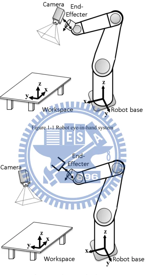
Figure 1-1 Robot eye-in-hand system ... 2

Figure 1-2 Robot eye-to-hand system ... 2

Figure 1-3 D-H parameters. ... 9

Figure 2-1 Overview of an eye-to-hand system with a laser pointer. ... 16

Figure 2-2 The laser beam with respect to the end-effector. ... 16

Figure 2-3 Projection of parallel laser beams on a plane. ... 18

Figure 2-4 Intersection of a laser beam and a plane. ... 20

Figure 3-1 Overview of an eye-to-hand system with a laser pointer. ... 28

Figure 3-2 Projection of laser beams on one plane ... 30

Figure 3-4 Projection of a end-effector translating vector along laser direction on a plane ... 34

Figure 4-1 Overview of an eye-to-hand system with a line laser module. ... 45

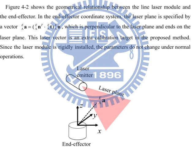
Figure 4-2 The laser plane with respect to the end-effector. ... 46

Figure 4-3 Projected laser stripes and virtual crossing points. ... 49

Figure 4-4 Projection of an end-effector translating vector along a laser plane on a working plane ... 50

Figure 5-1 The system configuration and coordinate relationship ... 57

Figure 5-2 The kinematics of last link with a laser pointer. ... 58

Figure 6-1 Overview of hardware of experiment. ... 62

Figure 6-2 Side view of simulation setups of the proposed method (Top) and the Dornaika and Horaud’s method (Bottom). ... 63

Figure 6-3 Relative errors with respect to the noise level. ... 65

Figure 6-4 Relative errors with respect to the number of samples. ... 66

Figure 6-5 Experimental setup. ... 67

Figure 6-6 Extrinsic results. ... 68

Figure 6-7 Relative errors with respect to the image pixel noise level. ... 70

Figure 6-8 Three different calibration references on the hand... 71

Figure 6-9 Relative errors of f , rotation, and translation with respect to noise u levels added in image pixel position. ... 72

Figure 6-10 Relative errors of f , rotation, and translation with respect to noise levels u added in robot hand translation. ... 73

(13)

Figure 6-11 Relative errors of f , rotation, and translation with respect to noise levels u

added in robot hand orientation. ... 74

Figure 6-12 Relative errors of f , rotation, and translation with respect to mixed u noise levels. ... 75

Figure 6-15 Extrinsic results. ... 78

Figure 6-16 Relative errors of closed-form solution with respect to the noise level. .. 81

Figure 6-17 Relative errors of nonlinear optimization with respect to the noise level. ... 81

Figure 6-20 Calibrated geometric relationships. ... 85

Figure 6-21 Average position error with respect to ... 87

(14)

List of Tables

Table 6-1 Results with real data of different number of samples ... 68

Table 6-2 The types of added noises ... 71

Table 6-3 Results of using Camera Calibration Toolbox for Matlab ... 78

Table 6-6 Kinematic parameters of simulation ... 86

(15)

List of Notations

Common Notations:

[

, ,

]

T

C = x y zC C C

p : Position in the camera coordinate system {C}

[

, ,

]

T

B = x y zB B B

p : Position in the robot base coordinate system {B}

[ ]

u v, T =

m : Image position

[

u v, ,1

]

T

=

m : Homogeneous coordinate of an image position

0 0 0 0 0 1 u c u v f f u f v α ⋅     =      

K : Camera intrinsic matrix

u

f : Focal length in u axis of a camera v

f : Focal length in v axis of a camera

c

α : Skew coefficient of a camera

0

u : Principal point in u axis of a camera

0

v : Principal point in v axis of a camera

1 2

{ , }κ κ : Radial distortion parameters of a camera

1 2

{ , }ρ ρ : Tangential distortion parameters of a camera

[

]

T

r = x zC C y zC C

x : Ray direction from the camera 1 T

T r =  r 

x x : Homogeneous coordinate of a ray direction from the camera

Πn : Plane normal vector

(16)

B

Πa : Plane pose

Λu : Unit vector of the laser beam

Λt : Position of the laser beam

b

aR : Rotation matrix from a frame to b frame

b

at : Translation vector from a frame to b frame

b

aT: Transformation matrix from frame a to frame b

n

a : Length of n-th link n

d : Normal offset of n-th link n

α : Twist angle of n-th link n

θ : Joint angle of n-th link H: Homogeneous matrix

i

h : i-th row of H

λ : Scalar factor of a homogeneous matrix

1 N

w w

 

=  

w  : Scales of a combination according to an end-effector movement

P: Number of plane poses

N: Number of end-effector translations

M : Number of end-effector orientations

K: Number of end-effector movements P: Projecting matrix

L

d : Distance from the laser origin to the projected point C

(17)

Chapter 2

,

m n

j : The n-th translating vector of the end-effector under the m-th orientation

,

m n

i : Moving vector of a laser spot corresponding to jm n,

[

0 1 2 3

]

T q q q q q = : Quaternion vector

Chapter 3

, , p m n

j : The n-th translating vector of the end-effector under the m-th orientation and the p-th plane pose

, ,

p m n

i : Moving vector of a laser spot corresponding to jp m n, ,

0 0 0 0 0 0 1 u v f f     =      

F : Camera intrinsic matrix composed of two focal lengths

Chapter 4

Λn : Normal vector of the laser plane

Λt : Position of the laser plane

Λa : Laser plane pose

, ,

p m n

k : The n-th translating vector of the end-effector under the m-th orientation and the p-th plane pose

i: Translating vector of a virtual cross point j : Translating vector of a virtual cross point

Chapter 5 {

1,..., 4N 4

}

S = s s + : The set of calibration parameters

[

1

]

T N

θ θ

=

(18)

Chapter 1 Introduction

Hand-eye coordination systems provide reliability and flexibility for complex tasks, in which the eye is a camera and the hand is a robot manipulator. Hand-eye coordination systems can be classified based on two camera configurations: eye-in-hand and eye-to-hand systems. A camera mounted on the end-effector (eye-in-hand), as shown in Figure 1-1, can be maneuvered to observe a target in detail. However, with a global view, a static camera (eye-to-hand), as shown in Figure 1-2, can detect scene changes more easily. Most works consider one configuration for a visual servo. Flandin et al. [1] described cooperation between eye-in-hand and eye-to-hand configurations to achieve both advantages. For position based visual servoing, camera calibration and hand-eye calibration are necessary. Since the pose of control points is estimated from their projections on a camera image, positioning error of a target may be significant due to inaccurate camera parameters. Furthermore, the end-effector positions maybe biased due to errors in the geometrical relationship. Notably, such errors can be eliminated by observing the end-effector directly. However, control points on the end-effector and target can often not be observed simultaneously, making it impossible to ensure positioning accuracy of the visual servo system [2]. Therefore, increasing calibration accuracy of robot hand-eye system still remains a major challenge in robotics. Calibrations often performed to maximize performance in such systems, including robot calibration, camera calibration, hand/eye calibration, and robot/workspace calibration.

(19)

Figure 1-1 Robot eye-in-hand system

(20)

1.1 Overview of Calibration of a Hand-Eye System

1.1.1 Hand-Eye Calibration

Hand-eye calibration of the eye-in-hand configuration has been discussed for several decades, with many solutions to estimate parameters accurately. While assuming that the camera is well calibrated, most works focus on calibrating geometrical relationships by utilizing a 3D object, 2D pattern, non-structured points, or just a point. Jordt et al. [35] categorized hand/eye calibration methods depending on the type of calibration reference. Based on their results, the following discussion summarizes four various approaches.

(1) Hand-eye calibration methods using 2D pattern or 3D object [3]-[32]

Most hand/eye calibration methods adopt a reference object with known dimensions or a standard calibration object. Features such as corners or circles on the calibration object are extracted in the images. Each feature is related to a position in the reference coordinate system. The camera pose can then be determined by inversely projecting the features in an image in the camera calibration stage. From this viewpoint, using a 2-D pattern is similar to using a 3-D one. The classical approaches to hand/eye calibration solve the transformation equation in the form, AX=XB, as first introduced by Shiu and Ahmad [3][7]. Tsai and Lenz [4][8] developed the closed-form solution by decoupling the problem into two stages: rotation and translation. Quaternion-based approaches, such as those developed by Chou and Kamel [5], Zhuang and Roth [10], and Horaud and Dornaika [16], lead to a linear form to solve rotation relationships. To avoid error propagation from the rotation stage to the translation stage, Zhuang and Shiu [12] developed a nonlinear optimization method with respect to three Euler angles of a rotation and a translation vector. Horaud and Dornaika [16] also applied a nonlinear optimization method to solve the rotation quaternion and the translation vector simultaneously. Albada et al. [17] considered robot calibration based on the camera calibration method by using a 2-D pattern. Daniilidis and Bayro-Corrochano [19][22] developed a method of representing a rigid transformation in a unit dual quaternion to solve rotation and translation relationships simultaneously. While simultaneously considering hand/eye and robot/world problems, Zhuang et al. [13] introduced the transformation chain in the

(21)

general form, AX=YB, and presented a linear solution based on quaternions and the linear least square method. Similarly, Dornaika and Horaud [21] included a closed-form solution and a nonlinear minimization solution. Hirsh et al. [23] developed an iterative approach to solve this problem. Li et al. [32] used dual quaternion and Kronecker product to solve it. The method of Strobl and Hirzinger [30] requires only orthogonal conditions in grids, which relaxes the requirement for patterns with precise dimensions.

(2) Hand-eye calibration methods using a single point [11], [33]-[35]

Wang [11] pioneered a hand/eye calibration procedure using only a single point at an unknown position. Pure translation without rotating the camera to observe the point yields a closed-form solution for the rotational relationship. Once the rotation is obtained, the translation relationship is solved via least squares fitting. Similar works such as [34] and [35] include finding camera intrinsic parameters. Gatla et al. [33] considered the special case of pan-tilt cameras attached to the hand.

(3) Hand-eye calibration methods using non-structured features [36]-[38]

This category can be considered an extension of using a single point. Rather than using a specific reference, the method of Ma [36] uses feature points of unknown locations in the working environment and determines the camera orientation by using three pure translations. By moving the camera without rotating, the focus of expansion (FOE) is determined by the movements of points in the images where the relative translation is parallel to a vector connecting the optical center and the FOE point. Directions of the three translations in the camera frame are related to the direction of hand movement in the robot frame. Based on such relationships, the camera orientation relative to the end-effector can be calculated. After the orientation is obtained, the camera position with respect to the robot can be obtained by analyzing the general motions. Similarly, Wei et al. [37] computed the initial parameters and developed an automatic motion planning procedure for optimal movement to minimize parameter variances. The work of Andreff et al. [38] was based on the structure-from-motion (SfM) method. It provided a linear formulation and several solutions for combining specific end-effector motions.

(22)

Optical flow data implicit the information of camera motion. To extract the relative pose from the flows and motions, Malm and Heyden [39]-[40] developed a method by pure translation followed by rotation around an axis. This category can be regarded as a unique case of using non-structured features.

While addressing the eye-in-hand and eye-to-hand configurations for visual servoing, Staniak and Zieliński [41] analyzed how calibration errors influence the control. Calibration of the eye-to-hand configuration for static camera has seldom been discussed since the transformation can be in the same form of eye-in-hand configuration. Most of the above methods are applicable to either eye-in-hand or eye-to-hand configurations. Dornaika and Horaud [21] presented a formulation to deal with the calibration problems for the both configurations, indicating that these two problems are identical. However, this identity is applicable only when the robot hand can be viewed with the eye-to-hand camera. This limits installation flexibility and potential applications. An eye occasionally fails to see a hand due to various requirements. For instance, to sort products on a moving conveyor, the camera is often placed at a distance from the arm to compensate for image processing delay and avoid interference when tracking targets on a rapidly moving conveyor belt. In catching ball systems, e.g., [44], cameras focus on the region of the initial trajectory of the ball and may not see the arm. Sun et al. [45] developed a robot-world calibration method using a triple laser device. Despite enabling calibration of the eye-to-hand transformation when the camera cannot see the arm, their method requires a uniquely designed triple-laser device, thus limiting the flexibility of system arrangement. Moreover, the spatial relationship from the working plane to camera must also be known in advance.

1.1.2 Camera Calibration

Since the camera calibration is fundamental in machine vision, there are rich literatures and resources on camera calibration. The direct linear transformation (DLT) (Abdel-Aziz and Karara [74] and Shapiro [75]) is applied to camera calibration to obtain linear solution. Bacakoglu and Kamel [76] adopted the DLT method and the nonlinear estimation, and developed methods to refine homogeneous transformation between the two steps. Methods based on DLT method basically need a 3D reference.

(23)

Tsai [77] developed a radial alignment constraint (RAC) based method using a 2D pattern. Zhuang et al. improved the Tsia’s RAC method and utilized robot mobility to deal with multiple planes. Zhang [50] provided a flexible method which can handle data of different poses of a planar pattern and doesn’t need any robot or linear table. An excellent toolbox named Camera calibration toolbox for Matlab (Bouguet [56]) based on Zhang’s method [50] is available online and is used in this work.

Most work on calibration of a hand-eye system is done by separating camera calibration and hand-eye calibration, subsequently causing error propagation. In many industrial applications, a camera must be recalibrated frequently. Camera calibration requires reference objects that could be a 3-D object [49], a 2-D pattern [50][51], or a 1-D bar [52]. However, in an environment that humans cannot easily enter to place a reference object, separating the calibration might become inefficient. Hence, Ma [36] developed a method that combines the two calibrations into one process when considering this problem for an active vision system.

1.1.3 Robot Calibration

Calibration of the geometrical parameters of a manipulator is important to ensure the accuracy of the end-effector position. The inaccuracy factors include assembly misalignments, tolerance of mechanical parts, and joint offset. Further, mechanical wear and temperature variation due to long-term operation will also induce drifts of the parameters. To maintain consistent performance, it is often necessary to calibration the manipulator even when it is in production line. As a result, cost-effective and easy-to-use calibration tools and methods are beneficial to enhance the efficiency of manipulator usage in industry.

Many studies of the kinematic identification and calibration were done [57]-[59]. Kinematic calibration methods generally consisted of four processes: kinematic modeling, measurement, identification, and correction [57]. High-accuracy laser interferometer is used for measuring the end-effector position, and then the calibrated parameters were obtained by applying nonlinear least square method [60] and neural networks [61]. The high-accuracy laser interferometer could guarantee tiny measurement error to achieve more accurate kinematic parameters. Rauf et al. [62] used a partial pose measurement device for kinematic calibration of parallel

(24)

manipulators. Renaud et al. [63] used a low-cost vision-based measuring device, which included a calibration board and a camera, to capture the end-effector pose and then calibrated the parallel manipulators. Another vision-based kinematic calibration uses the camera type 3D measurement device to capture the position of an infrared LED mounted on the end-effector [64]. In these vision-based methods, the manipulator must locate in the view of the camera.

In Newman and Osbom’s method, the manipulator was controlled to move along the laser line using an optical quadrant detector [65]. A laser pointer mounted on the end-effector is pointed to the position sensitive detector for workspace calibration [66] and kinematic calibration [67]. Park et al. [68] estimated the kinematic errors by using a structured laser module, a stationary camera, and they introduce a method based on the derived Jocabian matrices, and an extended Kalman filter. Two laser pointers beamed on the screen, and the camera measured an accurate position of two laser spots on the screen. In this setting (laser pointer/camera/plane), the arrangement for calibration is quite free as long as the laser pointer mounted on the manipulator is projected on the plane which is visible to the camera.

1.2 System Models and Parameters for Calibration

This section introduces the models and parameters of an eye-to-hand system for calibration, including intrinsic and extrinsic parameters of the camera, geometrical relationships between the camera and the robot, and geometrical relationships of the working plane in relation to the robot base coordinate system.

1.2.1 Camera Model

The camera model used is the pin-hole type with considering lens distortion. A 2D position in an image is denoted as m=

[ ]

u v, T, and its homogeneous coordinate is defined as m=

[

u v, ,1

]

T . A 3D position in the camera frame is denoted as

[

, ,

]

T C = x y zC C C p . 1 d d x y     = ⋅       m K with 0 0₀ 0 0 1 u c u v f f u f v α ⋅     =       K (1-1)

(25)

where K, the intrinsic matrix, including two focal lengths (f ,u f ), two principal v points (u ,0 v ), and a skew coefficient 0 αc, and

(

)

2 2 2 4 1 2 1 2 2 ₂ 1 2 2 ( 2 ) 1 ( 2 ) 2 r r r r d r r r d _r _r _{r r} x y x x y _y _{x y} ρ ρ κ κ ρ ρ  ₊ ₊      = + + +    + +    _ _ x x x x x (1-2) where

[

]

T r = x zC C y zC C

x is the ray direction from the camera, κ1 and κ2 are

radial distortion parameters, and ρ1 and ρ2 are tangential distortion parameters

(Brown [48]).

1.2.2 Eye-to-hand Transformation

The rigid transformation from one coordinate system to another coordinate is determined by a rotation matrix R and a translation vector t. A point a_{p in the a} frame is transformed into the b frame via

b b a b

a a

= ⋅ +

p R p t (1-3)

where R is a 3×3 rotation matrix and tis a 3×1 translation vector. The rotation matrix can be derived by the direction cosine matrix, ( , , )Rθ φ ϕ , and its rotation sequence is Z-Y-X, where θ is z-axis rotation, φ is y-axis rotation, and ϕ is x-axis rotation. In general, the robot base coordinate system is identical to the world coordinate system for the overall system in the following context. Transformation from the end-effector frame to the robot base frame is by a rotation matrix B

ER and a translation vectorB

Et, and they can be derived from robot forward kinematics. The relationships between the robot base and the camera are denoted as B B

C C

 

 R | t, and

these relationships are parts of the calibration target. 1.2.3 Planar Workspace Pose

Another calibration target is the pose of the workspace, which is a plane. The plane is defined by a normal vector B

Πn and a point ΠBt on the plane in the robot base

coordinate system. A plane in space has three degrees of freedom, and can be generally defined using the following vector.

( )

B B T B B

Πa= Πn ⋅Πt nΠ . (1-4)

(26)

satisfy the constraint,

( ) 0

B T B B

Πa p - aΠ = (1-5)

1.2.4 Manipulator Kinematics

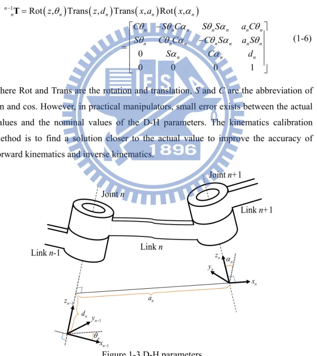
The D-H method [70] provides a standard method to write the kinematics of a manipulator. The D-H matrix of the n-th link includes four link parameters: the link length an, the normal offset dn, the angle of twist αn, and joint angle θn. As shown in Figure 1-3, the transformation matrix from frame n to frame n-1 is defined with D-H parameters as

(

)

(

)

(

)

(

)

1 _{Rot ,} _{Trans ,} _{Trans ,} _{Rot ,}

0 0 0 0 1 n n n n n n n n n n n n n n n n n n n n n n n z z d x a x C S C S S a C S C C C S a S S C d θ α θ θ α θ α θ θ θ α θ α θ α α − ₌ −    ₋    =       T (1-6)

where Rot and Trans are the rotation and translation, S and C are the abbreviation of sin and cos. However, in practical manipulators, small error exists between the actual values and the nominal values of the D-H parameters. The kinematics calibration method is to find a solution closer to the actual value to improve the accuracy of forward kinematics and inverse kinematics.

Figure 1-3 D-H parameters. n x n z n y Joint n Joint n+1 Link n Link n+1 Link n-1 n α 1 − n y 1 − n x θn 1 − n z an n d

(27)

1.3 Outline of Proposed Methods

1.3.1 Hand-Eye-Workspace Calibration using a Single Beam Laser

This work proposes a calibration method that can calibrate the relationships among the robot manipulator, the camera and the workspace. The method uses a laser pointer rigidly mounted on the manipulator and projects the laser beam on the work plane. Nonlinear constraints governing the relationships of the geometrical parameters and measurement data are derived. The uniqueness of the solution is guaranteed when the camera is calibrated in advance. As a result, a decoupled multi-stage closed-form solution can be derived based on parallel line constraints, line/plane intersection and projective geometry. The closed-form solution can be further refined by nonlinear optimization which considers all parameters simultaneously in the nonlinear model. Computer simulations and experimental tests using actual data confirm the effectiveness of the proposed calibration method and illustrate its ability to work even when the eye cannot see the hand. Only a laser pointer is required for this calibration method and this method can work without any manual measurement. In addition, this method can also be applied when the robot is not within the camera field of view. 1.3.2 Simultaneous Hand-Eye-Workspace and Camera Calibration using

a Single Beam Laser

This work presents a novel calibration technique capable of calibrating camera intrinsic parameters and hand-eye-workspace relations simultaneously. In addition to relaxing the requirement of a precise calibration reference under manipulator accuracy, the proposed method functions when the hand is not in the view field of the eye. The calibration method utilizes a laser pointer mounted on the hand to project laser beams onto a planar object, which can be the working plane. The collected images of laser spots must adhere to certain nonlinear constraints established by each hand pose and the corresponding plane-laser intersection. This work also introduces calibration methods for two cases in which single plane and multiple planes are used. A multistage closed-form solution is derived and serves as the initial guess to the nonlinear optimization procedure that minimizes the errors globally, allowing the proposed calibration method to function without manual intervention. The

(28)

effectiveness of the proposed method is verified by comparing with existing hand-eye calibration methods via simulation and experiments using an industrial manipulator. 1.3.3 Simultaneous Hand-Eye-Workspace and Camera Calibration using

a Line Laser

This work develops a novel calibration method for simultaneously calibrating the intrinsic parameters of a camera and the hand-eye-workspace relationships of an eye-to-hand system using a line laser module. Errors in the parameters of a hand-eye coordination system lead to errors in the position targeting in the control of robots. To solve these problems, the proposed method utilizes a line laser module that is mounted on the hand to project laser beams onto the working plane. As well as calibrating the system parameters, the proposed method is effective when the eye cannot see the hand and eliminates the need for a precise calibration pattern or object. The collected laser stripes in the images must satisfy nonlinear constraints at each hand pose. A closed-form solution is derived by decoupling nonlinear relationships based on the homogeneous transform and parallel plane/line constraints. A nonlinear optimization, which considers all parameters simultaneously without error propagation problem, is to refine the closed-form solution. This two-stage process can be executed automatically without manual intervention. The effectiveness of the proposed method is verified via computer simulation and experiments, and the simulation reveals that the line laser is more efficient than a single point laser.

1.3.4 Kinematic Calibration using a Single Beam Laser

This dissertation proposes a robot kinematic calibration system including a laser pointer installed on the manipulator, a stationary camera, and a planar surface. The laser pointer beams to the surface, and the camera observes the projected laser spot. The position of the laser spot is computed according to the geometrical relationships of line-plane intersection. The laser spot position is sensitive to slightly difference of the end-effector pose due to the extensibility of laser beam. Inaccurate kinematic parameters cause inaccurate calculation of the end-effector pose, and then the laser spot position by the forward estimation is deviated from the one by camera observation. For calibrating the robot kinematics, the optimal solution of kinematic parameters is obtained by minimizing the laser spot position difference between the

(29)

forward estimation and camera measurement via the nonlinear optimization method. The proposed kinematic calibration system is cost efficient and flexible for any manipulator. The proposed method is validated by simulation and experiments using real data.

1.4 Contributions of this Dissertation

The contribution of this dissertation is to propose and implement three new methods for calibration of a robot eye-to-hand system. The first one uses a single beam laser and the second one uses same device but can simultaneously calibrate the camera intrinsic parameters. The third one uses a line laser (a type of structure lasers). This dissertation also introduces a robot kinematic calibration method by using a laser pointer, a camera, and a plane. Contributions of this dissertation are listed as,

1. The calibration reference proposed is distinctly different from existing methods. The formulation and solution are both original since all existing calibration algorithms cannot apply. A major advantage of this approach is that the laser beam enables hand-eye calibration even when the eye cannot see the hand. In other words, this technique increases the working range of hand-eye coordination that provides installation flexibility and potential applications.

2. A closed-form solution is developed by decoupling nonlinear equations into linear forms. This enables automatic data collection and computation of all initial values which are used for subsequent nonlinear optimization to refine the estimation for higher accuracy. Hence, it is possible to implement self-calibration since there is no need to conduct manual measurement of objective parameters.

3. For eye-to-hand systems, the proposition to use a single beam laser relaxes the requirement of a precise calibration reference, such as chessboards, point grids, and horizontal patterns. This greatly reduces the system cost and potential errors induced by those references. This contribution is comparable to the work for eye-in-hand by Ma [36] where only a single fixed point in workspace is needed. 4. Based on the proposed method, any projected patterns of laser beam on a fixed

object seen by the camera can be used as a calibration point. This offers the potential to use this method for on-line monitoring of robot accuracy and fault without the need of costly installation.

(30)

5. The proposed robot kinematic calibration is a step forward improvement of the work in [68] to reduce the number of laser pointer to 1, hence pre-calibration of a laser module is not necessary.

1.5 Dissertation Organization

The remainder of this dissertation is organized as follows. The hand-eye-workspace calibration method using a single beam laser is introduced in Chapter 2. Chapter 3 presents the simultaneous hand-eye-workspace and camera calibration method using a single beam laser. Chapter 4 presents the simultaneous hand-eye-workspace and camera calibration method using a line laser. Next, the kinematic calibration method is provided in Chapter 5. Chapter 6 shows the experimental results by simulations and using real data. Finally, conclusion and future work are drawn in Chapter 7.

(31)

Chapter 2 Hand-Eye-Workspace Calibration using a

Single Beam Laser

2.1 Introduction

A general eye-to-hand calibration method using a laser pointer mounted on the end-effector was proposed in (Hu and Chang [47]). This chapter first considers the case in which intrinsic parameters of the camera are already known. As a result, only one plane is needed and if the working plane is assigned, this method enables simultaneous eye-hand-workspace calibration. Ghosh et al.’s method [79] considers calibrating the workspace together, but their method needs another sensor and has to assume that the working plane and the horizontal plane of the robot base are parallel. Our proposed method takes the advantage of robot's mobility and dexterity.

By manipulating the robot to project the laser beam on the plane, a batch of related image positions of light spots is extracted from camera images. Since the laser is mounted rigidly and the plane is fixed, the geometrical parameters and measurement data must obey certain nonlinear constraints, and the parameter solutions can be estimated accordingly. A closed-form solution is developed by decoupling nonlinear equations into linear forms to compute all initial values. Therefore, the proposed calibration method does not require manual estimation of unknown parameters. To achieve high accuracy, a nonlinear optimization method that considers all parameters at a time is then implemented to refine the estimation. This approach doesn’t need

(32)

manual installation of a pattern or an object in the workspace; hence, it will enable fully automatic calibration.

The remainder of this dissertation is organized as follows. First an overview of the approach is given. The basic idea of using system redundant information to achieve calibration is presented. Following that are details of the closed-form solution and nonlinear optimization based on the geometrical constraints. A recommended procedure of implement of this approach is provided. The proposed method is then discussed with experimental results obtained by simulations and using real data. The results are compared with the results of using Dornaika and Horaud’s method [21] in the simulations. Finally, a conclusion is given.

2.2 Preliminaries

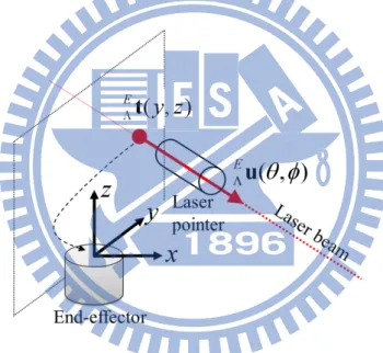
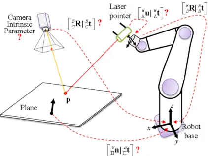
The objective of calibration is to reduce systematic errors by correcting the parameters. The geometrical relationships using a laser pointer to calibrate an eye-to-hand system is illustrated here. Figure 2-1 shows the overall configuration of an eye-to-hand system, in which a laser pointer is attached to the end-effector for calibration and a working plane is in front of the camera.

Figure 2-2 shows the relationships between the laser pointer and the end-effector. In the coordinate system of the end-effector, the direction of the laser beam is described as a unit vectorE

Λu , which has two degrees of freedom and can be denoted

by Euler angles as

cos sin sin sin cos T

E E_θ E_φ E_θ E_φ E_φ

Λu=  Λ Λ Λ Λ Λ  (2-1)

where E_θ [0,2 )_π

Λ ∈ is the z-axis rotation angle and ΛEφ∈[0, ]π is the angle between

z-axis and E

Λu . Without loss of generality, let the laser origin ΛEt be the point at

which the laser beam intersects the x-y plane of the end-effector coordinate system, i.e.,

[0 ]

E E _{y z} T

Λt = Λ . (2-2)

Otherwise, let E E[_x 0 _z]T

Λt = Λ or ΛEt=ΛE[x y 0]T . These additional laser

parameters must then be calibrated. Since the laser pointer is rigidly installed, these parameters do not change under normal operation.

(33)

Figure 2-1 Overview of an eye-to-hand system with a laser pointer.

Figure 2-2 The laser beam with respect to the end-effector.

In summary, the calibration targets are hand/eye/workspace relationships and additional laser installation parameters, and camera intrinsic parameters are known a prior. The unknown relationships are labeled with question marks in Figure 2-1. In this system, three methods can be used to calculate a laser spot 3D position which the laser beam is projected onto the plane and that laser spot is captured by the camera.

1) Intersection of the laser beam and plane:

The 3D location of a laser point on a plane is derived via the principle of line/plane intersection. The geometrical constraint is

(34)

( B B B )T B 0 L

d Λu+ Λt− Πa ⋅Πa= (2-3)

where d is the distance from the laser origin to the projected point and L B B T B L B T B d Π Λ Π Λ Π − ⋅ = ⋅ a t a u a . (2-4)

Hence, the 3D position of the laser spot is described as

B B B

spot =dLΛ + Λ

p u t. (2-5)

2) Intersection of the plane and ray from the camera:

A laser spot is projected onto an image taken by the camera. The ray direction, denoted as x , from the origin of the camera frame to the laser spot can be obtained r using the pixel position by applying the inverse intrinsic matrix and the undistortion method. According to the principle of line/plane intersection, the geometrical constraint is (B C B B )T B 0 CR⋅dC xr +Ct− Πa ⋅Πa= (2-6) where C T 1 T r =  r  x x . Then, ( ) B B T B C C B C T B C r d Π Π Π − ⋅ = ⋅ a t a R x a. (2-7)

Hence, the 3D position of the laser spot is

B B C B

spot =dC⋅C r + C

p R x T. (2-8)

3) Triangulation of the laser beam and ray from the camera: PositionB

spot

p can also be determined by triangulation of the laser beam and the camera ray. This position, which is the intersection of two lines, is

B B B B B

spot =dLΛ + Λ =dC r +C

p u t x t. (2-9)

This leads to the equation:

- L B B B B r C C d d Λ Λ    _{ }= −  u x _{ } t t (2-10)

which can be solved by least squares method.

This analysis indicates the existence of redundant information in this system configuration. The positional differences of the same point derived via the different methods are caused by systematic errors and/or noisy measurements. This implies that the systematic parameters can be estimated by tuning these parameters to reduce the

(35)

differences of positions, either 3D positions or 2D image positions.

A closed-form solution is proposed followed by an optimization solution. The optimization problem, which is described later, is nonlinear. To avoid local minimum and to accelerate convergence, accurate initial values are needed. The closed-form solution is derived by exploring the arrangements in the setup. Since no prior guess of parameters is needed, the proposed method can run automatically.

2.3 Closed-form solution

Some parts of the closed-form solution are achieved by translating, but not rotating, the end-effector. This pure translational motion can decompose the problem into linear forms according to the constraints of parallel laser beams.

Several orientations of the end-effector with the laser pointer are performed. Under the m-th orientation, the end-effector is translated, but not rotated, along several vectors, jm n, ’s, and the laser spot on the plane moves along corresponding vectors,

,

m n

i ’s, as shown in Figure 2-3. In the end, the orientations of laser beams corresponding with different hand poses determine the geometric dimensions of the overall system.

(36)

The step-by-step of this closed-form solution is clearly described in detail as follows.

1) Calculate the ray directions of all points:

Each projected laser spot is located in an image, and its direction from the camera is obtained by calculating its inverse projection. With the camera intrinsic parameters, for any point in an image, the ray direction x can then be derived accordingly. r 2) Find homogeneous matrixes, each having an unknown scale factor:

Suppose the end-effector moves along a direction (without rotation) that is a linear combination of N translating vectors (jm n, vectors). The laser spot will move along a

vector that is the same linear combination of corresponding vectors (im n, vectors).

Specifically, under m-th rotation and k-th translation, the laser spot is at position

1 , , ,1 , , , 1 1 r m k m k m m m N m N m k m k w z z w     ⋅     _ __ _ =_ _ = _ _{ }= _{  }     _ _   x w x H i  i t  (2-11)

where w , n = 1~N are scales of a combination according to end-effector movement, n

and H is a homogeneous matrix . Let m h be the i-th row of i H. A solution for the

homogeneous matrix can then be obtained by DLT method (Hartley and Zisserman [54]). That is 1 2 3 T T T T k r k T T T k r k x y    _{ } _ ⋅ =_ _{ } _=  _{  }   H H h w 0 - w Q x h 0 0 w - w _h . (2-12)

For K points, dimension of Q is (2K)×(3N +3), and a unique solution H x exists ifH H

Q is ranked 3N+2. The solution is the eigenvector corresponding to the smallest eigenvalue of the matrix T

H H

Q Q . According to (2-13), the solution has an unknown scalar factor λ, and

,1 ,

ˆ ˆ

m =λm m =λm m m N m

H H i  i t (2-13)

Scalar factors of M orientations (λm, m = 1~M) are obtained in the following steps. 3) Find the normal vector of the plane w.r.t the camera:

(37)

orthogonal to these vectors, i.e., C TΠn i⋅ m n, =0 for n = 1~N, m = 1~M. The resulting equations are 1,1 , ˆ ˆ T C T M N Π     =_ _⋅ =     n n i Q x n 0 i  (2-14)

For N×M vectors, the dimension of Q is (NM)×3, and a unique solution n x exists n

if the ˆim n, ’s are not parallel. If the numbers of translating vectors in each orientation

are identical, Equation (2-14) has N×M equations. The solution is the eigenvector corresponding to the smallest eigenvalue of the matrix T

n n

Q Q and is normalized to a unit vector.

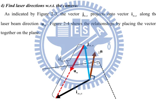
4) Find laser directions w.r.t. the camera:

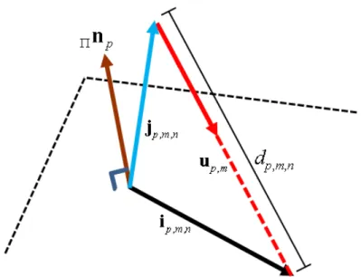
As indicated by Figure 2-3, the vector jm n, projects onto vector im n, along the

laser beam direction um. Figure 2-4 shows the relationships by placing the vectors together on the plane.

Figure 2-4 Intersection of a laser beam and a plane. Therefore, , , , m n = m n+dm n m i j u (2-15) where , , T m n m n T m d Π Π ⋅ = − ⋅ j n u n , which is equivalent to , , , T m m n m m n T m n m Π Π  ⋅  = ⋅ =_ − _⋅ ⋅   u n i G j I j u n (2-16)

(38)

, , ,

C C C C C B

m n m⋅ m n m B⋅ ⋅ m n

i = G j = G R j . (2-17) Let a transformation matrix be defined as

1 ₁ 2 2 3 3 ˆ ˆ ˆ ˆ C C C C C m m B B C m m   _ _   _ _ = ⋅ =   _ _   _ _       g _g G = g G R g R g g (2-18) Equation (2-17) can be rewritten as

1 , , , 2 , , , ₃ ˆ ˆ ˆ T B T m n B T T C m n m m n m n m n B T _T m n m         =_ _  = =       _ _ g, g j 0 0 A x 0 j 0 g b i 0 0 j _g . (2-19)

The N translating vectors in m-th orientation form

1 1 ,m N _m N _m       ₌              g A b x A b   . (2-20)

The Bjm n, ’s are from the manipulator commands and Cˆim n, ’s replacing Cim n, ’s in

(2-20) are obtained from previous procedure ((2-13)). The solution is calculated by least squares method and is rearranged into a 3×3 matrix, which is proportional to

ˆ

m

G with a scalar 1λm. This matrix is denoted as Gm =Gˆm λm . According to (2-20), at least three non-coplanar robot translations are required to obtain a unique solution.

The rotation term can be eliminated algebraically by multiplying Gm with its transpose. Let /

(

T

)

m = m λm m⋅ Π u u u n . According to (2-16) and (2-17),

(

)

(

2

)

T T T T T T T m m = m⋅Π − m⋅Π ⋅ m⋅Π − m⋅Π ⋅Π ⋅ m+ m m G G  u n I u n u n u n n u u u  (2-21)

Each element on the left side equal to relative element on the right side forms a quadratic equation of three arguments that are three elements of um. Since the matrix

T m m

G G  is symmetric, it contains six quadratic equations and their coefficients are composed of the elements of the normal vector Πn . The solution of these equations

is um. Normalizing um to a unit vector gives the laser direction um at the m-th orientation in the camera frame.

(39)

Since rotation between the robot base frame and the camera frame is unique, all vectors at different hand orientations are subject to this relation. From (2-18),

, ,

ˆT B C T a m =C a m

g R g for a = 1~3 and m = 1~M. Rotation B

CR represented by a unit quaternion is applied to obtain a linear form of this equation (Horn[55]). The quaternion is generally defined as q q q= 0+ 1i+q2j+q3k and can also be written in a

vector

[

₀ ₁ ₂ ₃

]

T q q q q q = . Let _v_{ˆ [0}₌ _gˆ_]T_and _v₌_[0 C_{g ,}_]T -1 ˆ = ⊗ ⊗ v q v q (2-22)

where ⊗ represents quaternion multiplication and q is the inverse of the -1 quaternion. Equation (2-22) is equal to

(

)

ˆ⊗ − ⊗ = E( )ˆ −W( ) = v q q v v v q 0 (2-23) where 0 1 2 3 1 0 3 2 2 3 0 1 3 2 1 0 - - -( ) -v v v v v v v v E v v v v v v v v       =       v and 0 1 2 3 1 0 3 2 2 3 0 1 3 2 1 0 - - -( ) -v v v v v v v v W v v v v v v v v       =       v

The equation for all vectors rotating from camera frame to robot base frame is,

1,1 1,1 3, 3, _{(12 ) 4} ˆ ( ) ( ) ˆ ( ) ( ) B C M M _M E W E W _×  −    =_ _ =  ₋    q q v v Q x q 0 v v  (2-24)

The solution is the eigenvector corresponding to the smallest eigenvalue of the matrix T

q q

Q Q and is normalized to satisfy B T B 1

Cq qC = . The rotation matrix from the camera coordinate system to the robot base coordinate system is then obtained from

2 2 2 3 1 2 3 0 1 3 2 0 2 2 1 2 3 0 1 3 2 3 1 0 2 2 1 3 2 0 2 3 1 0 1 2 1 2 2 2( ) 2( ) 2( ) 1 2 2 2( ) 2( ) 2( ) 1 2 2 B B C C q q q q q q q q q q q q q q q q q q q q q q q q q q q q q q  − − + −    = _ − − − + _  ₊ ₋ ₋ ₋    R . (2-25)

6) Find the laser direction w.r.t the end-effector:

The laser emitter is rigidly attached on the end-effector and the laser beam direction is E

Λu relative to the end-effector frame. The laser beam direction at the m-th hand

orientation in the camera frame is

C C B E

m B E m Λ

u = R R u. (2-26) Hence, the M orientations lead to an equation,

基於雷射光束投影之機器人手眼校正方法

國 立 交 通 大 學

電機與控制工程研究所

博

士

論

文

基於雷射光束投影之機器人手眼

校正方法

Calibration of Robot Eye-to-Hand System

Using Laser Beam Projection

研 究 生：張永融

指導教授：胡竹生 教授

基於雷射光束投影之機器人手眼校正方法

Calibration of Robot Eye-to-Hand System

Using Laser Beam Projection

研

究 生：張永融 Student：Yung-Jung Chang

指導教授：胡竹生

Advisor：Jwu-Sheng Hu

國

立 交 通 大 學

電

機 與 控 制 工 程 研 究 所

博

士 論 文

A Dissertation

Submitted to Department of Electrical and Control Engineering

College of Electrical Engineering and Computer Science

National Chiao Tung University

in partial Fulfillment of the Requirements

for the Degree of

Doctor of Philosophy

in

Electrical and Control Engineering

July 2012

Hsinchu, Taiwan, Republic of China

基於雷射光束投影之機器人手眼校正方法

研究生：張永融

指導教授：胡竹生 博士

國立交通大學電機與控制工程研究所博士班

摘要

Calibration of Robot Eye-to-Hand System

Using Laser Beam Projection

Department of Electrical and Computer Engineering

National Chiao-Tung University

Abstract

致 謝

Contents

List of Figures

List of Tables

List of Notations

Common Notations:

[

]

[

]

[ ]

[

]

[

]

Chapter 2

[

]

Chapter 3

Chapter 4

Chapter 5

{

}

[

]

Chapter 1

Introduction

1.1 Overview of Calibration of a Hand-Eye System

1.1.1 Hand-Eye Calibration

1.1.2 Camera Calibration

1.1.3 Robot Calibration

1.2 System Models and Parameters for Calibration

[ ]

國立交通大學

研究生：張永融

指導教授：胡竹生教授

究生：張永融 Student：Yung-Jung Chang

立交通大學

機與控制工程研究所

士論文

指導教授：胡竹生博士

致謝