壓電材料迴轉體與楔形板幾何引致電彈奇異性之探討

(1)

i

行政院國家科學委員會補助專題研究計畫

■ 成果報告 □期中進度報告

壓電材料迴轉體與楔形板幾何引致電彈奇異性之探討

計畫類別：

■

個別型計畫 □整合型計畫

計畫編號：NSC 100－2221－E－009－093－MY2

執行期間：100 年 8 月 1 日至 100 年 10 月 31 日

計畫主持人：黃炯憲

計畫參與人員：胡政甯、詹志偉、劉靖俞、李承哲、郭芳琳、黃旭進、

王裕鈞、楊維莘

成果報告類型(依經費核定清單規定繳交)：□精簡報告

■

完整報告

本成果報告包括以下應繳交之附件：

□赴國外出差或研習心得報告一份

□赴大陸地區出差或研習心得報告一份

□出席國際學術會議心得報告及發表之論文各一份

□國際合作研究計畫國外研究報告書一份

執行單位：國立交通大學

中華民國 102 年 11 月 10 日

(2)

An eigenfunction expansion approach is combined with a power series solution technique to establish the asymptotic solutions for geometrically induced electroelastic singularities in piezoelectric bodies of revolution and wedges, with arbitrary direction of polarization. The asymptotic solutions are obtained by directly solving the three-dimensional equilibrium and Maxwell’s equations in terms of displacement components and electric potential. Since the direction of polarization can be arbitrary in space, the in-plane components of displacement and electric field are generally coupled with the out-of-plane components, and the coupling substantially complicates the solutions. The correctness of the proposed solutions are confirmed by comparing the present results with the published results obtained by assuming axisymmetric deformation or generalized plane deformation. The numerical results related to singularity orders are shown for bodies of revolution and wedges that comprise a single material (PZT-4 or PZT-5H) or bonded piezo/piezo (PZT-4/PZT-5H) or piezo/isotropic elastic (PZT-4/Al or PZT-5H/Al) materials. The numerical results concerning the order of the singularity are expressed in graphic form, and are shown herein for the first time.

Key words: electroelastic singularities, piezoelectric bodies of revolution, piezoelectric wedges, three-dimnsional asymptotic solutions, eigenfunction expansion approach

(4)

摘要本研究透過特徵函數展開法配合級數解建立電磁彈性迴轉體與楔形體之三維電磁彈奇異性漸近解。直接求解於以位移與電勢表示的三維力平衡與馬克斯威爾(Maxwell) 方程組之漸近解。由於考慮材料具任意之極化方向，造成面外與面內之位移與電場彼此耦合，導致求解之困難度。透過與文獻中假設軸對稱變形或廣義平面變形所得結果比較，驗證本研究所得解之正確性◦根據漸近解，將探討有關於極化方向、幾何形狀、材料種類與邊界條件對於電磁彈性與壓電迴轉體與楔型體奇異性階數之影響；其中迴轉體與楔形體可為單一壓電材料(PZT-4 與 PZT-6B) 、壓電/各向同向性彈性材料(PZT-4/Si 或 PZT-6B/Si)或雙壓電材料(PZT-4/PZT-6B)。所得數值結果以圖表示，本研究所得均首見於文獻◦ 關鍵詞：奇異性、壓電迴轉體、壓電楔形體、三維漸近解、特徵函數展開法

(5)

1

I. Introduction 1.1 Literature Review

Piezoelectric material is a widely used, smart or intelligent material, because of the intrinsic effects of coupling between electric fields and mechanical deformation. Piezoelectric materials have been extensively applied in actuators, resonators, oscillators, conductors and sensors. The most interesting feature of piezoelectric materials is that they can serve not only as actuators, providing driving signals, but also as sensors for smart structures. In the practical applications, electroelastic singularities are commonly observed at a sharp corner or because of discontinuity in material properties. Accordingly, either local mechanical failure or dielectric failure can occur at a sharp corner. Understanding of the electroelastic singularity behaviors of piezoelectric wedges is essential to optimize the design of piezoelectric devices and further advance smart material technology. Furthermore, an accurate numerical analysis of problems that involve stress singularities depends on knowledge of such stress singularity behaviors. The two typical geometries that are commonly considered in the literature on geometrically induced stress singularities are wedges and bodies of revolution.

The stress singularities in a wedge have been comprehensively examined. Since Williams (1952a) pioneered the investigation of stress singularities of plates under extension, many studies of stress singularities in wedges of a single material or multiple materials have been carried out, based on the plane strain or stress assumption (e.g. Williams, 1952b; Hein and Erdogan, 1971; England, 1971; Bogy and Wang, 1971; Dempsey and Sinclair, 1981; Ying and Katz, 1987) or three-dimensional elasticity theory (e.g. Hartranft and Sih, 1969; Chaudhuri and Xie, 2000). Geometrically induced stress singularities in plates of a single material and multiple materials have also been extensively studied using classical thin plate theory (e.g. Williams, 1952c; Williams and Owens, 1954), first-order shear deformation plate theory (e.g. Burton and Sinclair, 1986; Huang, 2002a; Huang, 2003; Saidi et al., 2010; McGee and Kim, 2005), and third–order plate theory (Huang, 2002b).

Numerous analyses of stress singularities for elastic bodies of revolution are also available. Making an assumption of axisymmetric deformation, Zak (1964) utilized the Love stress approach (Love, 1927) to investigate geometrically induced stress singularities in bodies of revolution that were made of a single material, while Li et al. (1998, 2000) adopted the Love stress approach and Boussinesq's solution (Timoshenko and Goodier, 1970) respectively, to obtain the stress field near the bond edge of a bi-material body of revolution. Ting et al. (1985) presented eigenfunctions at a singular point of a body of revolution made of transversely isotropic material. Without assuming axisymmetric deformation, Huang and Leissa (2007) presented three-dimensional sharp corner displacement functions for bodies of revolution, and further studied the geometrically induced stress singularities in bimaterial bodies of revolution (Huang and Leissa, 2008).

(6)

A few studies of the geometrically-induced electroelastic singularities at the vertex of a piezoelectric wedge (Fig. 2.1) are based on the assumption that all physical quantities under consideration depend on the planar coordinates. Based on the plane strain assumption (ε ,_zz

zy

ε , ε , andzx E , which are defined in Chapter 2, equal zero), Xu and Rajapakse (2000) z

extended Lekhnitskii’s complex potential functions for in-plane stresses and electric displacement components to examine the electroelastic singularities at the vertex of a piezoelectric wedge that has a direction of polarization on the x-y plane (see Fig. 2.1). Based on an assumption of generalized plane deformation, Chue and Chen (2002) presented a decoupled formulation of piezoelectric elasticity and applied it to examine the stress singularities near the apex of a rectilinearly polarized piezoelectric wedge, considering its direction of polarization in the x-y plane or along the z-axis. Hwu and Ikeda (2008) proposed an extended Stroh formulation in an (x, y) coordinate system by considering a generalized plane strain and short circuit (ε = and _zz 0 E_z = ) and presented numerical results for the 0 electroelastic singularities at the vertices of piezoelectric wedges and multi-material wedges with the directions of polarization in the x-y plane. Because different plane assumptions were made in these three cited papers, they employed different constitutive laws in their solutions. Notably, Xu and Rajapakse (2000) treated the piezoelectric material as transversely isotropic material as they began to develop solutions while Chue and Chen (2002) and Hwu and Ikeda (2008) treated piezoelectric material as generally anisotropic. The solutions of Xu and Rajapakse (2000) include only in-plane physical quantities, while those of Chue and Chen (2002) and Hwu and Ikeda (2008) included in-plane and out-of-plane physical quantities. Following the assumptions in Chue and Chen (2002), Chen, Chu and Lee (2004) employed the extended Lekhnitskii formulation to determine the eletroelastic singularity behaviors near the apex of a piezoelectric wedge that was polarized in the radial, circular, or axial direction. Chu and Chen (2003) applied the Mellin transform to determine anti-plane stress singularities in a bonded bi-material piezoelectric wedge. Neglecting all out-of-plane physical quantities, Shang and Kitamura (2005) utilized a modified version of the general solution that was developed by Wang and Zheng (1995) and Shang et al. (2005) to investigate the stress singularities at the interface edge of a wedge made of two piezoelectric materials with the direction of polarization parallel to the x-axis.

A review of the literature reveals only two investigations that considered eletroelastic singularities in a piezoelectric body of revolution, based on axisymmetric deformation assumptions. To perform stress singularity analysis of axisymmetric piezoelectric bonded structures, Xu and Mutoh (2001) adopted the general solutions for coupled equations for piezoelectric material that was developed by Ding et al. (1996), while Li and Sato (2002) extended the method proposed by Ting et al. (1985) for an elastic material. These solutions

(7)

3

consist of four and three quasi-harmonic functions, respectively. In these two works, the direction of polarization of the piezoelectric material was assumed to be along the axis of revolution.

1.2 Purposes of Research

The main purpose of the present research is to develop an asymptotic solution for the eletroelastic singularities in a piezoelectric body of revolution and wedge without any restrictions on the direction of polarization of the material. When a piezoelectric material is considered to be transversely isotropic, and the axis of material symmetry is not parallel to the axis of revolution, the assumption of axisymmetric deformation is no longer valid. Since the direction of polarization can be arbitrary in space, the in-plane components of displacement and electric field are generally coupled with the out-of-plane components. An eigenfunction expansion approach combined with a power series method is adopted to solve the equilibrium and Maxwell’s equations in terms of mechanical displacement components and electric potential. The correctness of the proposed solution is confirmed by comparing the present results with the published results in cases in which the direction of polarization is along some special directions. Analyses are performed on bodies that comprise a single piezoelectric material (PZT-4 or PZT-5H), bonded piezo/piezo (PZT-4/PZT-5H) or piezo/isotropic elastic (PZT-4/Al or PZT-5H/Al) materials. The effects of geometry of body, polarization orientation, material type(s) and boundary conditions on the singularity orders are comprehensively examined. The numerical results concerning the order of the singularity are expressed in graphic form, and are shown herein for the first time.

(8)

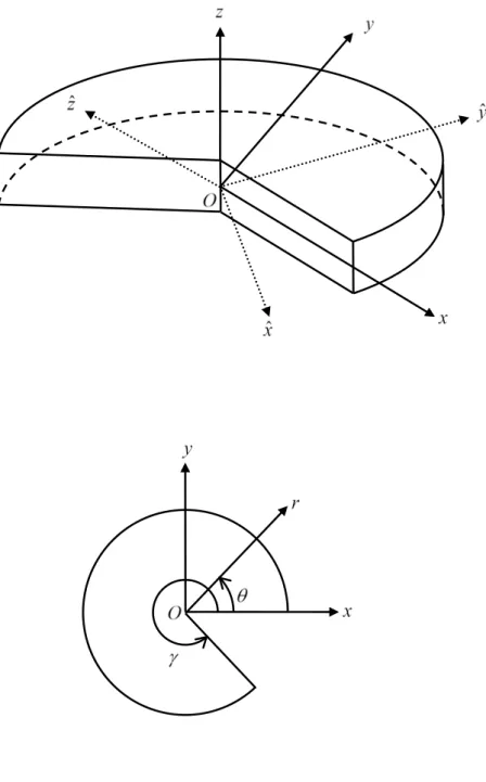
II Asymptotic Solutions for a Wedge 2.1 Basic Formulation

Consider a rectilinearly anisotropic piezoelectric wedge that is polarized in the ˆz

direction, as presented in Fig. 2.1. The constitutive equations of the piezoelectric material are expressed in the material coordinate system (ˆ ˆ ˆx, y, z), as

{ }

[ ]

{ }

_ˆ

[ ]

T

{ }

_ˆ

ˆ ˆc eˆ E

σ = ε − , (2.1a)

{ }

_Dˆ ₌

[ ]

_e_ˆ

{ }

_ε_ˆ ₊

[ ]

_η_ˆ

{ }

_Eˆ _, _(2.1b)

where

{ }

σˆ =

{

σ_xx_{ˆ ˆ} σ_{ˆ ˆ}_yy σ_ˆˆ_zz σ_yz_ˆ_ˆ σ_ˆ_zx_ˆ σ_ˆˆ_xy

}

T is the stress vector;

{ }

εˆ =

{

ε_xx_{ˆ ˆ} ε_{ˆ ˆ}_yy ε_zz_ˆˆ 2ε_ˆ_yz_ˆ 2ε_ˆ_zx_ˆ 2ε_xy_ˆˆ

}

T is the strain vector;

{ } {

Dˆ = D_ˆ_x D_y_ˆ D_z_ˆ

}

Tis the electric displacement vector;

{ } {

Eˆ = E_ˆ_x E_ˆ_y E_z_ˆ

}

T is the electric field vector, and

[ ]

ˆc ,

[ ]

ˆe and

[ ]

ηˆ are the mechanical elastic constant matrix, the piezoelectric constant matrix

and the dielectric constant matrix, respectively.

It is easy to solve for the eletroelastic singularities at the vertex of the wedge in the cylindrical coordinate system (r,θ,z) given in Fig. 2.1. In the cylindrical coordinate system, the equilibrium and Maxwell’s equations in terms of stress components (σ ) and electric _ij displacements (D ) without body force and charges are _i

(

)

1 0, rr r rr rz r r z r θθ θ σ σ σ σ σ θ − ∂ ∂ ∂ + + + = ∂ ∂ ∂ (2.2a) 1 2 0, r z r r r z r θ θθ θ θ σ σ σ σ θ ∂ ₊ ∂ ₊∂ ₊ ₌ ∂ ∂ ∂ (2.2b) 1 0, z rz zz rz r r z r θ σ σ σ σ θ ∂ ∂ ₊ ₊∂ ₊ ₌ ∂ ∂ ∂ (2.2c)

( )

1 1 0, r z rD D D r r r z θ θ ∂ ∂ ∂ + + = ∂ ∂ ∂ (2.2d)

The constitutive equations of the piezoelectric material in the cylindrical coordinate system are

{ }

σ =

[ ]

c

{ }

ε −

[ ]

e E

{ }

, (2.3a)

{ }

[ ]

T

{ }

[ ]

{ }

D = e ε + η E , (2.3b)

(9)

5

{ } {

}

T r z D = D D_θ D ,

{ } {

E = E_r E_θ E_z

}

T,

[ ]

11 12 13 14 15 16 12 22 23 24 25 26 13 23 33 34 35 36 14 24 34 44 45 46 15 25 35 45 55 56 16 26 36 46 56 66 c c c c c c c c c c c c c c c c c c c c c c c c c c c c c c c c c c c c c         =             ,

[ ]

11 12 13 14 15 16 21 22 23 24 25 26 31 32 33 34 35 36 e e e e e e e e e e e e e e e e e e e     =       ,

[ ]

1112 1222 1323 13 23 33 η η η η η η η η η η     =       . (2.4)

The components of

[ ]

c ,

[ ]

e and

[ ]

η are related to the components of

[ ]

ˆc ,

[ ]

ˆe and

[ ]

ηˆ , respectively; and are functions of θ and depend on the direction cosines between (ˆ ˆ ˆx, y, z)

and (x, y, z). These relations are given in Appendix I.

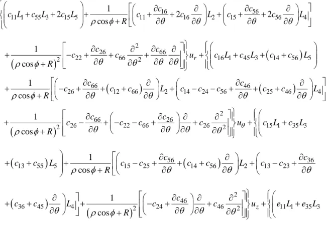
Substituting strain-displacement relations and electric field-potential relations into Eqs. (2.3) and (2.4) enables the stress components and electric displacements to be expressed in terms of mechanical displacement components (u , u_r _θ and u ) and electric potential (_z ϕ ),

given in Appendix II. Substituting those expressions into Eqs. (2.2) yields the governing equations in terms of mechanical displacement components and electric potential as

2 2 2 2 16 56 66 11 2 55 2 11 15 2 2 16 2 56 c c c c c c c c c r z θ r r θ r z θ r θ r r θ r θ z  ∂ ₊ ∂ ₊ ₊∂  ∂ ₊ ₊∂  ∂ ₊∂ ∂ ₊ ∂ ₊ ∂      ∂ ∂  ∂  ∂  ∂  ∂ ∂ ∂ ∂ ∂ ∂ ∂  2 2 2 2 26 66 15 22 66 2 2 16 2 45 2 26 1 2c c c c u_r c c c c r z θ θ r r z θ r r   ∂   ∂ ∂ ∂ ∂ ∂   ∂ + + −_ + + _ _ +_ + + −_ + _ ∂ ∂  ∂ ∂    ∂ ∂  ∂  ∂

(

)

2

(

)

2 46 26 14 24 56 22 66 2 12 66 25 46 c c c c c c c c c c c r z r r r r z θ θ θ θ θ ∂ ∂ ∂ ∂ ∂ ∂     +_ − − + _ + −_ − + _ + + + + ∂ ∂ ∂ ∂ ∂ ∂ ∂ ∂    

(

)

2 66 2 2 2 56 14 56 26 26 2 2 15 2 35 2 15 25 1 c c c c c c u c c c c r z θ θ r θ r z θ r r   ∂   ∂ ∂ ∂ ∂ ∂   ∂ + + +_ − + _ _ +_ + +_ − + _ ∂ ∂  ∂ ∂    ∂ ∂  ∂  ∂

(

)

2

(

)

2 36 46 13 23 24 2 14 56 36 45 c c c c c c c c c r z r r r r z θ θ θ θ θ ∂ ∂ ∂ ∂ ∂ ∂     +_ − + _ + −_ + _ + + + + ∂ ∂ ∂ ∂ ∂ ∂ ∂ ∂    

(

)

2 2 2 2 16 13 55 46 2 2 z 11 2 35 2 11 12 e c c c u e e e e r z r θ r z θ r r   ∂ ∂ ∂ ∂ ∂   ∂ + + + _ +_ + +_ − + _ ∂ ∂ ∂   ∂ ∂  ∂  ∂

(10)

(

)

2

(

)

2 36 26 31 32 22 2 16 21 25 36 e e e e e e e e e r z r r r r z θ θ θ θ θ ∂ ∂ ∂ ∂ ∂ ∂     +_ − + _ + −_ + _ + + + + ∂ ∂ ∂ ∂ ∂ ∂ ∂ ∂    

(

e31 e15

)

2 e26 2 2 2 0 r z r θ ϕ  ∂ ∂ + + + _ = ∂ ∂ _{∂ } , (2.5a) 2 2 25 26 12 16 2 45 2 2 16 26 2 56 24 22 66 2 c c c c c c c c c c c r z θ r r θ r z θ r θ  ∂ ₊ ∂ ₊ ₊ ₊∂  ∂ ₊ ₊ ₊∂  ∂ ₊ ₊ ₊∂  ∂        _∂ _∂ _ _∂ _ _∂ _ _∂ _ _∂ _ _∂ _ _∂ 

(

)

2

(

)

2

(

)

2 22 2 12 66 25 46 56 14 26 26 2 2 1 r c c c c c c c c c u r r θ r θ z r z θ θ r   ∂  ∂ ∂ ∂ ∂ + + + + + + +_ + + _ _ ∂ ∂ ∂ ∂ ∂ ∂ _ ∂ ∂ _{ } 2 2 2 26 24 22 66 2 44 2 66 46 2 2 26 c c c c c c c c r z θ r r θ r z θ r θ r r θ  ∂ ∂  ∂  ∂  ∂  ∂ ∂  ∂ ∂ +_ + +_ + _ +_ + _ +_ _ + ∂ ∂  ∂  ∂  ∂  ∂  ∂  ∂ ∂ ∂  2 2 2 2 2 26 25 24 46 66 22 2 2 56 2 34 2 56 1 2c 2c c c c u c c 2c c r θ z r z θ θ r θ r z θ   ∂   ∂ ∂ ∂ ∂ ∂ ∂   + + + −_ − + _ _ +_ + +_ + _ ∂ ∂ ∂ ∂  ∂ ∂    ∂ ∂  ∂ 

(

)

2

(

)

2 23 24 36 46 2 25 46 23 44 2c c c c c c c c r r θ r z θ r θ r r θ r θ z ∂ ∂ ∂   ∂   ∂ ∂ ∂ × +_ + _ +_ + _ + + + + ∂  ∂  ∂  ∂  ∂ ∂ ∂ ∂ ∂

(

)

2 2 2 2 12 32 36 45 24 2 2 z 16 2 34 2 2 16 2 36 e e c c c u e e e e r z r θ r z θ r r θ r z   ∂ ∂ ∂ ∂ ∂ ∂   ∂   ∂ + + + _ +_ + +_ + _ +_ + _ ∂ ∂ ∂   ∂ ∂  ∂  ∂  ∂  ∂

(

)

2

(

)

2

(

)

2 2 22 26 2 12 26 24 32 36 14 22 2 2 0 e e e e e e e e e r r r r z r z r ϕ θ θ θ θ θ  ∂ ∂ ∂ ∂ ∂ ∂   +_ + _ + + + + + + + _ = ∂ ∂ ∂ ∂ ∂ ∂ ∂ ∂ ∂    , (2.5b)

(

)

2 2 45 46 14 15 2 35 2 15 25 23 55 24 2 14 56 c c c c c c c c c c c c r z θ r r θ r z θ r θ  ∂ ₊ ∂ ₊ ₊ ₊∂  ∂ ₊ ₊ ₊∂  ∂ ₊ ₊∂  ∂ ₊ ₊        _∂ _∂ _ _∂ _ _∂ _ _∂ _ _∂ _ _∂ _ _∂ 

(

)

(

)

2 2 2 2 2 2 24 45 36 55 13 46 2 2 56 2 34 2 1 r c c c c c c u c c r r θ r θ z r z θ θ r r z  ∂   ∂ ∂ ∂ ∂ ∂ ∂ × + + + + +_ + _ _ +_ + ∂ ∂ ∂ ∂ ∂ ∂ _ ∂ ∂ _ _ _ ∂ ∂

(

)

2

(

)

46 44 24 45 36 46 2 25 46 44 23 c c c c c c c c c c r r r z r r r θ θ θ θ θ ∂ ∂ ∂ ∂ ∂ ∂ ∂       +_ _ +_ − + _ + −_ + _ + + + + ∂ ∂  ∂  ∂  ∂  ∂ ∂ ∂  

(

)

2 2 2 2 2 46 45 45 36 24 2 2 55 2 33 2 55 1 c c c c c u c c c r θ z r z θ θ r θ r z θ r r   ∂   ∂ ∂ ∂ ∂ ∂ ∂   ∂ × + + + −_ + _ _ +_ + +_ + _ ∂ ∂ ∂ ∂  ∂ ∂    ∂ ∂  ∂  ∂

(11)

7 2 2 2 2 34 44 35 2 2 45 2 34 2 35 44 2 2 z c c c c c c c u r z r r r r z r z r θ θ θ θ θ θ  ∂ ∂ ∂ ∂ ∂ ∂ ∂ ∂     +_ + _ +_ _ + + + + _ ∂ ∂  ∂  ∂ ∂ ∂ ∂ ∂ ∂ ∂ ∂   

(

)

2 2 2 34 14 24 15 2 33 2 15 35 2 25 14 e e e e e e e e e r z θ r r θ r z θ r θ r r θ  ∂ ∂  ∂  ∂  ∂  ∂ ∂  ∂ ∂ +_ + +_ + _ +_ + _ +_ _ + + ∂ ∂  ∂  ∂  ∂  ∂  ∂  ∂ ∂ ∂ 

(

e34 e23

)

2

(

e35 e13

)

2 e24 2 2 2 0 r θ z r z r θ ϕ  ∂ ∂ ∂ + + + + + _ = ∂ ∂ ∂ ∂ _{∂ } , (2.5c) 2 2 25 26 21 11 2 35 2 11 12 15 32 22 2 e e e e e e e e e e r z θ r r θ r z θ r θ  ∂ ₊ ∂ ₊ ₊ ₊∂  ∂ ₊ ₊ ₊∂  ∂ ₊ ₊∂  ∂        ∂ ∂  ∂  ∂  ∂  ∂  ∂  ∂ 

(

)

2

(

)

2

(

)

2 22 2 2 16 21 25 36 15 31 26 2 2 16 2 1 r e e e e e e e e u e r r θ r θ z r z θ θ r r  ∂   ∂ ∂ ∂ ∂ ∂ + + + + + + +_ + _ _ +_ ∂ ∂ ∂ ∂ ∂ ∂ _ ∂ ∂ _ _ _ ∂

(

)

2 2 26 24 22 34 2 14 36 26 2 12 26 e e e e e e e e e z θ r r θ r z θ r θ r r θ ∂ ∂ ∂ ∂   ∂   ∂   ∂ ∂ + +_ _ +_ − + _ + −_ + _ + + ∂  ∂  ∂  ∂  ∂  ∂  ∂ ∂ ∂

(

)

2

(

)

2 26 2 2 2 24 32 14 36 22 2 2 15 2 33 2 1 e e e e e e u e e r θ z r z θ θ r θ r z   ∂   ∂ ∂ ∂ ∂ ∂ + + + + + −_ + _ _ +_ + ∂ ∂ ∂ ∂ _ ∂ ∂ _ _ _ ∂ ∂

(

)

2

(

)

2 25 23 24 15 13 2 14 25 23 34 e e e e e e e e e r r r z r r r r z θ θ θ θ θ θ ∂ ∂ ∂ ∂ ∂ ∂ ∂ ∂       +_ + _ +_ + _ +_ _ + + + + ∂ ∂ ∂ ∂  ∂  ∂ ∂ ∂ ∂ ∂    

(

)

2 2 2 2 12 22 13 35 24 2 2 z 11 2 33 2 11 2 e e e u r z r r z r r r η η η η η θ θ θ θ   ∂ ∂ ∂ ∂ ∂ ∂   ∂   ∂ + + + _ −_ + +_ + _ +_ _ ∂ ∂ ∂   ∂ ∂  ∂  ∂  ∂  ∂ 2 2 2 2 23 13 2 12 2 23 2 13 22 2 2 0 r z r r r z r z r η η η η η η ϕ θ θ θ θ  ∂ ∂ ∂ ∂ ∂ ∂   +_ + _ + + + + _ = ∂ ∂ ∂ ∂ ∂ ∂ ∂ ∂ ∂    . (2.5d)

2.2. Construction of Asymptotic Solution

To determine the asymptotic solution of Eqs. (2.5) as r approaches zero, the mechanical displacement components and electric potential in the double series can be conveniently expanded as follows;

(

)

( )

_{( )}

0 0 ˆ , , m n m , r n m n u r θ z rλ U θ z ∞ ∞ + = = =

∑∑

, (2.6a)

(12)

(

)

( )

_{( )}

0 0 ˆ , , m n m , n m n u_θ r θ z rλ V θ z ∞ ∞ + = = =

∑∑

, (2.6b)

(

)

( )

_{( )}

0 0 ˆ , , m n m , z n m n u rθ z rλ W θ z ∞ ∞ + = = =

∑∑

, (2.6c)

(

)

( )

_{( )}

0 0 ˆ , , m n m , n m n r z rλ z ϕ θ ∞ ∞ + θ = = =

∑∑

Φ , (2.6d)

where the characteristic values λ are assumed to be constants and can be complex _m numbers. The real part of λ has to be positive to satisfy the regularity conditions for _m mechanical displacement components and electric potential at r=0 (such as finite displacement and electric potential at r=0).

Substituting Eqs. (2.6) into Eqs. (2.5) and carefully arranging the resulting equations yields

(

)(

)

( )

₍

₎

( ) ( )

₍

₎

2 16 66 11 11 16 0 0 ˆ ˆ ˆ 1 2 m m m m n n m m n m n m m n c c U rλ c λ n λ n U c λ n U c λ n θ θ θ ∞ ∞ + − = =  _ _∂ _ _∂ _∂ + + − + + + + + + ×  _ _∂ _ _∂ _∂ 

∑∑

( ) ( )

₍

₎₍

₎

( )

₍

₎

( ) 2 26 66 22 66 2 16 26 ˆ ˆ ₁ ˆ ˆ m m m m n n m m n m n U c c c c U c λ n λ n V c λ n V θ θ θ θ   ∂ _{+ −} ₊∂ ₊ ∂ ₊ ₊ _{+ −} _{+ −} ₊∂  ₊     ∂  ∂ ∂   ∂  ( )

(

)(

)

( ) 2 ( )

₍

₎

26 66 22 66 12 66 26 26 2 15 ˆ ˆ ˆ m m m n n m n m c V V c c c c c λ n c c V c λ n θ θ θ θ θ   ∂ ∂ ∂ ∂ ∂   + −_ − + _ + + + +_ − + _ + + × ∂ ∂ ∂ ∂ ∂    

(

)

( ) 56

₍

₎

( ) 46 ( )

₍

₎₍

₎

( ) 15 25 24 14 56 ˆ ˆ ˆ ˆ 1 m m m m _n _n m n m n m c c W W n W c c n W c c c n λ λ λ θ θ θ θ ∂ ∂ ∂ ∂     + − +_ − + _ + + − +_ _ + + + ∂ ∂ ∂ ∂     ( )

(

)(

)

( )

₍

₎

( ) ( ) 2 16 26 46 2 11 11 12 22 ˆ ˆ ˆ ˆ 1 m m m m n n m m n m n W e e c e λ n λ n e e λ n e θ θ θ θ ∂  ∂   ∂ ∂Φ + + + + − Φ +_ − + _ + Φ + −_ + _ ∂  ∂   ∂  ∂

(

)(

)

( ) 2 ( ) 1 56 ( ) 2 ( )

(

)

16 21 26 2 15 56 15 ˆ ˆ ˆ ˆ 2 2 m m m m m n n n n n m m c U U e e n e r c c c n z z λ λ λ θ θ θ θ + −  ∂Φ ∂ Φ  ∂ ∂ ∂ + + + + _+ __ + _ + + + × ∂ ∂   ∂  ∂ ∂ ∂ ( ) ( )

(

)

2 ( )

(

)(

)

( )

(

)

46 14 24 56 25 46 14 56 36 45 ˆ m ˆ m ˆ m ˆm n n n n m U c V V V c c c c c c c n c c z θ z θ z λ z ∂ ₊ ₋ ₋ ₊∂ ∂ ₊ ₊ ∂ ₊ ₊ ₊ ∂ ₊ ₊ _×   ∂  ∂  ∂ ∂ ∂ ∂ ( ) ( )

(

)(

)

( ) ( )

(

)

2 36 36 13 23 13 55 31 32 25 36 ˆ m ˆ m ˆ m ˆ m n n n n m W c W W e c c c c n e e e e z z λ z z θ θ θ ∂ ₊ ₋ ₊∂ ∂ ₊ ₊ ₊ ∂ ₊ ₋ ₊∂ ∂Φ ₊ ₊ _×     ∂ ∂  ∂  ∂ ∂  ∂  ∂ ( )

(

)(

)

( ) ( ) ( ) ( ) ( ) 2 2 2 2 2 31 15 55 2 45 2 35 2 35 2 ˆ ˆ ˆ ˆ ˆ ˆ 0 m m m m m m m n n n n n n n m U V W e e n r c c c e z z z z z z λ λ θ +    ∂ Φ ₊ ₊ ₊ ∂Φ ₊ ∂ ₊ ∂ ₊ ∂ ₊ ∂ Φ ₌    _ _ ∂ ∂ ∂ _ _ ∂ ∂ ∂ ∂ _ (2.7a)

(13)

9

(

)(

)

( )

₍

₎

( ) ( ) 2 12 26 16 16 26 22 66 0 0 ˆ ˆ ˆ 1 2 m m m m n n m m n m n m n c U c rλ c λ n λ n U c c λ n U c c θ θ θ ∞ ∞ + − = = ∂ ∂  ₊ _{+ −} ₊ ₊ ₊∂  ₊ ₊ ₊ ₊       _ _∂ _ _ _∂ _ _∂ 

∑∑

(

)(

)

( ) 22 2 ( )

₍

₎₍

₎

( ) 22 ( ) 12 66 26 26 2 66 ˆ ˆ ˆ ₁ ˆ m m m m n n m n m m n U c c V c c λ n c c U c λ n λ n V θ θ θ θ θ   ∂ ∂ ∂ ∂ ∂ + + + +_ + + _ + + + − +_ _ ∂  ∂ ∂   ∂  ∂

(

)

( )

₍

₎

( ) 2 ( )

₍

₎

26 26 66 26 66 22 2 56 ˆ ˆ ₂ ˆ m m n m m n m n m c V c c λ n V c λ n c c V c λ n θ θ θ θ   ∂ ∂ ∂ ∂   +_ + _ + + + + −_ − + _ + + × ∂ ∂ ∂ ∂    

(

)

( ) 25

₍

₎

( ) 24 ( )

₍

₎₍

₎

( ) 56 46 25 46 ˆ ˆ ˆ ˆ 1 2 m m m m n n m n m n m c c W W n W c n W c c c n λ λ λ θ θ θ θ ∂ ∂ ∂ ∂     + − +_ + _ + +_ + _ + + + ∂  ∂  ∂ ∂   ( )

(

)(

)

( )

₍

₎

( ) ( ) 2 12 22 24 2 16 16 26 ˆ ˆ ˆ ˆ 1 2 m m m m n n m m n m n W e e c e λ n λ n e λ n e θ θ θ θ ∂  ∂   ∂ ∂Φ + + + + − Φ +_ + _ + Φ +_ + _ ∂  ∂   ∂  ∂

(

)(

)

( ) 2 ( ) 1 25 ( )

(

)

2 ( ) 12 26 22 2 56 24 25 46 ˆ ˆ ˆ ˆ 2 m m m m m n n n n n m c U U e e n e r c c c c z z λ λ θ θ θ θ + −  ∂Φ ∂ Φ  ∂ ∂ ∂ + + + + _+ __ + + _ + + ∂ ∂   ∂  ∂ ∂ ∂

(

)(

)

( ) 24 ( ) 2 ( )

(

)

( ) 23 56 14 46 24 46 36 ˆ ˆ ˆ ˆ 2 2 2 m m m m n n n n m m U c V V V c c c n c c c n c z z z z λ λ θ θ θ ∂  ∂ ∂ ∂ ∂  ∂  + + + +_ + _ + + + +_ + _× ∂  ∂  ∂ ∂ ∂ ∂  ∂  ( )

(

)

2 ( )

(

)(

)

( ) 32 ( )

(

)

2 ( ) 23 44 36 45 36 24 32 ˆ ˆ ˆ ˆ ˆ 2 m m m m m n n n n n m W W W e c c c c n e e e z θ z λ z θ z θ z ∂ ₊ ₊ ∂ ₊ ₊ ∂ ₊ ₊∂ ∂Φ ₊ ₊ ∂ Φ   ∂ ∂ ∂ ∂  ∂  ∂ ∂ ∂

(

36 14

)(

)

( ) 45 2 2( ) 44 2 2( ) 34 2 2( ) 34 2 2( ) ˆ ˆ ˆ ˆ ˆ 0 m m m m m m n n n n n n m U V W e e n r c c c e z z z z z λ λ ∂Φ  +  ∂ ∂ ∂ ∂ Φ  + + + _∂ + _ _∂ + _∂ + _∂ + _∂ _=    (2.7b)

(

)(

)

( )

₍

₎

( ) ( ) 2 14 46 15 15 25 24 0 0 ˆ ˆ ˆ 1 m m m m n n m m n m n m n c U c rλ c λ n λ n U c c λ n U c θ θ θ ∞ ∞ + − = = ∂ ∂  ₊ _{+ −} ₊ ₊ ₊∂  ₊ ₊ ₊       _ _∂ _ _ _∂ _ _∂ 

∑∑

(

)(

)

( ) 24 2 ( )

₍

₎₍

₎

( ) 46

₍

₎

14 56 46 2 56 ˆ ˆ ₁ ˆ m m m n m n m m n m U c c c c λ n c U c λ n λ n V λ n θ θ θ θ   ∂ ∂ ∂ ∂  + + + +_ + _ + + + − +_ _ + × ∂  ∂ ∂   ∂  ( ) 24 ( )

₍

₎₍

₎

( ) 46 2 ( )

₍

₎

46 25 46 24 2 55 ˆ ˆ ˆ ˆ m m m n n m n m n m V V c c V c c c λ n c V c λ n θ θ θ θ θ   ∂ ∂ ∂ ∂ ∂   + −_ + _ + + + + −_ + _ + + × ∂ ∂ ∂ ∂ ∂    

(

)

( ) 45

₍

₎

( ) 44 ( )

₍

₎

( ) 2 ( ) 55 45 44 2 ˆ ˆ ˆ ˆ ˆ 1 2 m m m m m n n n m n m n m c c W W W n W c n W c n c λ λ λ θ θ θ θ θ ∂ ∂ ∂ ∂ ∂     + − +_ + _ + +_ _ + + + ∂  ∂  ∂ ∂ ∂  

(

)(

)

( ) 14

₍

₎

( ) 24 ( )

₍

₎₍

₎

( ) 15 15 25 14 ˆ ˆ ˆ ˆ 1 m m m m n n m m n m n m e e e λ n λ n e λ n e e λ n θ θ θ θ ∂Φ ∂Φ ∂ ∂     + + + − Φ +_ + _ + Φ +_ _ + + + ∂ ∂ ∂ ∂    

(14)

( ) ( )

(

)

( )

(

)(

)

( ) 2 2 1 45 24 2 23 55 45 36 55 13 ˆ ˆ ˆ ˆ m m m m m n n n n n m c U U U e r c c c c c c n z z z λ _λ θ θ θ + −  ∂ Φ  ∂ ∂ ∂ ∂ + _+ __ + + _ + + + + + ∂   ∂  ∂ ∂ ∂ ∂ ( )

(

)

2 ( )

(

)(

)

( ) 34 ( ) 24 45 36 44 23 45 36 35 ˆ m ˆm ˆ m ˆ m n n n n m V V V c W c c c c c c c n c z z λ z z θ θ θ ∂ ∂ ∂ ∂ ∂ ∂     +_ − + _ + + + + + +_ + _ ∂ ∂ ∂ ∂ ∂ ∂ ∂     ( )

(

)

( ) ( )

(

)

( )

(

)(

)

2 2 34 34 35 35 34 23 35 13 ˆ ˆ ˆ ˆ 2 2 m m m m n n n n m m W W e c c n e e e e e n z λ z z z λ θ θ θ ∂ ∂  ∂ ∂Φ ∂ Φ + + + +_ + _ + + + + + × ∂ ∂ ∂  ∂  ∂ ∂ ∂ ( ) ˆ m n z  ∂Φ  ∂  ( ) ( ) ( ) ( ) 2 2 2 2 35 2 34 2 33 2 33 2 ˆ ˆ ˆ ˆ 0 m m m m m n Un Vn Wn n r c c c e z z z z λ +  ∂ ∂ ∂ ∂ Φ  + _ + + + _= ∂ ∂ ∂ ∂   (2.7c)

(

)(

)

( )

₍

₎

( ) ( ) 2 21 26 11 11 12 22 0 0 ˆ ˆ ˆ 1 m m m m n n m m n m n m n e U e rλ e λ n λ n U e e λ n U e θ θ θ ∞ ∞ + − = = ∂ ∂  ₊ _{+ −} ₊ ₊ ₊∂  ₊ ₊ ₊       _ _∂ _ _ _∂ _ _∂ 

∑∑

(

)(

)

( ) 22 2 ( )

₍

₎₍

₎

( ) 26

₍

₎

16 21 26 2 16 ˆ ˆ ₁ ˆ m m m n m n m m n m U e e e e λ n e U e λ n λ n V λ n θ θ θ θ   ∂ ∂ ∂ ∂  + + + +_ + _ + + + − +_ _ + × ∂  ∂ ∂   ∂  ( ) 22 ( )

₍

₎₍

₎

( ) 26 2 ( )

₍

₎

26 12 26 22 2 15 ˆ ˆ ˆ ˆ m m m n n m n m n m V V e e V e e e λ n e V e λ n θ θ θ θ θ   ∂ ∂ ∂ ∂ ∂   + −_ + _ + + + + −_ + _ + + × ∂ ∂ ∂ ∂ ∂    

(

)

( ) 25

₍

₎

( ) 24 ( )

₍

₎₍

₎

( ) 2 ( ) 15 14 25 24 2 ˆ ˆ ˆ ˆ ˆ 1 m m m m m n n n m n m n m e e W W W n W e n W e e n e λ λ λ θ θ θ θ θ ∂ ∂ ∂ ∂ ∂     + − +_ + _ + +_ _ + + + + ∂  ∂  ∂ ∂ ∂  

(

)(

)

( ) 12

₍

₎

( ) 22 ( )

₍

₎

( ) 11 11 12 ˆ ˆ ˆ ˆ 1 2 m m m m n n m n m n n m n n m n η η η λ λ η λ η λ θ θ θ θ ∂Φ ∂Φ ∂ ∂     − + + − Φ −_ + _ + Φ −_ _ − + ∂ ∂ ∂ ∂     ( ) ( )

(

)

( )

(

)(

)

( ) 2 2 1 25 22 2 15 32 25 36 15 31 ˆ ˆ ˆ ˆ m m m m m n n n n n m e U U U r e e e e e e n z z z λ η λ θ θ θ + −  ∂ Φ  ∂ ∂ ∂ ∂ − _+ __ + + _ + + + + + ∂   ∂  ∂ ∂ ∂ ∂ ( )

(

)

2 ( )

(

)(

)

( ) 23 ( ) 24 14 36 24 32 14 36 13 ˆ m ˆ m ˆ m ˆ m n n n n m V V V e W e e e e e e e n e z z λ z z θ θ θ ∂ ∂ ∂ ∂ ∂ ∂     +_ − + _ + + + + + +_ + _ ∂ ∂ ∂ ∂ ∂ ∂ ∂    

(

)(

)

( ) 23 ( ) 2 ( )

(

)

( ) 13 35 13 23 13 ˆ ˆ ˆ ˆ 2 2 m m m m n n n n m m W e e n n z z z z η λ η η η λ θ θ  ∂  ∂ ∂Φ ∂ Φ ∂Φ + + + −_ + _ − − + _ ∂  ∂  ∂ ∂ ∂ ∂ _ ( ) ( ) ( ) ( ) 2 2 2 2 35 2 34 2 33 2 33 2 ˆ ˆ ˆ ˆ 0 m m m m m n Un Vn Wn n r e e e z z z z λ +  ∂ ∂ ∂ _η ∂ Φ  + _ + + − _= ∂ ∂ ∂ ∂   (2.7d)

To investigate the behaviors of the solutions around r=0, only the parts of the solutions with the lowest order of r have to be considered. That is the solution corresponding to n=0 in Eqs. (2.7). Accordingly, the following equations must be solved.

(15)

11 ( )

( )

_{( )}

( )

_{( )}

( )

_{( )}

( )m m m m m m V p V p V p U p U p U 0 5 0 4 2 0 2 3 0 2 0 1 2 0 2 ˆ ˆ ˆ ˆ ˆ ˆ θ θ θ θ θ θ θ θ θ ∂ + ∂ + ∂ ∂ + + ∂ ∂ + ∂ ∂

( )

ˆ( )

( )

ˆ( )

( )

_ˆ( )

_{( )}

ˆ( )

_{( )}

ˆ( )

_{( )}

_ˆ( ) ₀ 0 11 0 10 2 0 2 9 0 8 0 7 2 0 2 6 _∂ + Φ = Φ ∂ + ∂ Φ ∂ + + ∂ ∂ + ∂ ∂ + m m m m m m p p p W p W p W p θ θ θ θ θ θ θ θ θ θ (2.8a) ( )

( )

_{( )}

( )

_{( )}

( )

_{( )}

( ) 2 2 0 0 0 0 1 2 0 3 4 5 0 2 2 ˆ ˆ ˆ ˆ ˆ ˆ m m m m m m V V U U q θ q θ V q θ q θ q θ U θ θ θ θ ∂ ₊ ∂ ₊ ₊ ∂ ₊ ∂ ₊ ∂ ∂ ∂ ∂

( )

2 0( )

( )

0( )

( )

_{( )}

2 ( )0

_{( )}

( )0

_{( )}

( ) 6 2 7 8 0 9 2 10 11 0 ˆ ˆ ˆ ˆ ˆ ˆ ₀ m m m m m m W W q θ q θ q θ W q θ q θ q θ θ θ θ θ ∂ ∂ ∂ Φ ∂Φ + + + + + + Φ = ∂ ∂ ∂ ∂ (2.8b) ( )

( )

_{( )}

( )

_{( )}

( )

_{( )}

( ) 2 2 0 0 0 0 1 2 0 3 4 5 0 2 2 ˆ ˆ ˆ ˆ ˆ ˆ m m m m m m W W U U r θ r θ W r θ r θ r θ U θ θ θ θ ∂ ₊ ∂ ₊ ₊ ∂ ₊ ∂ ₊ ∂ ∂ ∂ ∂

( )

2 0( )

( )

0( )

( )

_{( )}

2 ( )0

_{( )}

( )0

_{( )}

( ) 6 2 7 8 0 9 2 10 11 0 ˆ ˆ ˆ ˆ ˆ ˆ ₀ m m m m m m V V r θ r θ r θ V r θ r θ r θ θ θ θ θ ∂ ∂ ∂ Φ ∂Φ + + + + + + Φ = ∂ ∂ ∂ ∂ (2.8c) ( )

( )

_{( )}

( )

_{( )}

( )

_{( )}

( ) 2 2 0 0 0 0 1 2 0 3 4 5 0 2 2 ˆ ˆ ˆ ˆ ˆ ˆ m m m m m U U m s θ s θ s θ s θ s θ U θ θ θ θ ∂ Φ ₊ ∂Φ ₊ _{Φ +} ∂ ₊ ∂ ₊ ∂ ∂ ∂ ∂

( )

2 0( )

( )

0( )

( )

_{( )}

2 0( )

_{( )}

0( )

_{( )}

( ) 6 2 7 8 0 9 2 10 11 0 ˆ ˆ ˆ ˆ ˆ ˆ ₀ m m m m m m V V W W s θ s θ s θ V s θ s θ s θ W θ θ θ θ ∂ ∂ ∂ ∂ + + + + + + = ∂ ∂ ∂ ∂ (2.8d) Appendix III defines p , _i q , _i r , and _i s in Eqs. (2.8). _i

Equations (2.8) are a set of ordinary differential equations with variable coefficients that depend only on θ. The solutions to Eqs. (2.8) are independent of z. The exact closed-form solutions to Eqs. (2.8) are intractable, if they exist. The power series method can be directly adopted to develop a general solution for ordinary differential equations with variable coefficients. Very high-order terms must be considered to obtain an accurate solution and this requirement can cause numerical difficulties. To overcome these difficulties, a domain decomposition technique is used in conjunction with the power series method to establish a general solution of Eqs. (2.8).

The range of θ under consideration is first divided into a number of sub-domains (see Fig. 2.2). A series solution to Eqs. (2.8) is established in each sub-domain. Consequently, a general solution over the whole θ domain is constructed from these series solutions in the sub-domains by imposing the continuity conditions between each pair of adjacent sub-domains. This process is a very convenient means of constructing solutions that can be used to analyze multi-material wedges, which are also considered in this work.

(16)

To establish the power series solution for sub-domain i of θ, the variable coefficients in Eqs. (2.8) are expanded in terms of the power series of θ with respect to the middle point of the sub-domain, θ : _i

( )

(

)

∑

= − = K k k i i k j j p 0 θ θ µ θ ,

( )

(

)

∑

= − = K k k i i k j j q 0 θ θ ς θ ,

( )

_∑

( )

(

)

= − = K k k i i k j j r 0 θ θ ξ θ ,

( )

(

)

∑

= − = K k k i i k j j s 0 θ θ ϑ θ . (2.9)

Similarly, the solutions of Eqs. (2.8) in sub-domain i are expressed as

( )

_∑

( )

(

)

= − = J j j i i j m i A U 0 0 ˆ ˆ _θ _θ , ( )

_∑

( )

(

)

= − = J j j i i j m i B V 0 0 ˆ ˆ _θ _θ , ( )

_∑

( )

(

)

= − = J j j i i j m i C W 0 0 ˆ ˆ _θ _θ , ( )

_∑

( )

(

)

= − = Φ J j j i i j m i D 0 0 ˆ ˆ _θ _θ (2.10) Substituting Eqs. (2.9) and (2.10) into Eqs. (2.8) and carefully rearranging yields the following relations among the coefficients in Eqs. (2.10)

( )

_{( )}

( ) ( )

_{( )}

( ) ( )

_{( )}

( ) ( )

(

)(

)

(

)(

) ( )

(

( ) ( ) 1 2 3 0 2 6 0 2 9 0 2 3 2 0 1 ˆ ˆ ˆ ˆ ₂ ₁ ˆ 2 1 j i i i i i i i i i j j j j j k k k A B C D k k B j j µ µ µ − µ + + + + ₋ + =  − _ + + + = _{ } + + + _{+ }

∑

( )

( ) ( )

_{( )}

( ) ( )

)

₍

_{)( )}

( ) ( )

_{( )}

( ) ( )

₍

_{)( )}

( ) ( ) 6 2 9 2 1 1 2 4 1 0 ˆ ˆ j ₁ ˆ ˆ ₁ ˆ i i i i i i i i i i k k k k k j k j k j k j k j k k C D k A A k B µ ₋ ₊ µ ₋ ₊ µ ₋ ₊ µ ₋ µ ₋ ₊ =   + + __+

∑

_ + + + +

( )

( ) ( )

₍

_{)( )}

( ) ( )

_{( )}

( ) ( )

₍

_{)( )}

( ) ( )

_{( )}

( ) ( )

}

5 ˆ 1 7 ˆ 1 8 ˆ 1 10 ˆ 1 11 ˆ i i i i i i i i i i k k k k k j k B k j kC j kC k j k D j kD µ ₋ µ ₋ ₊ µ ₋ µ ₋ ₊ µ ₋  + + + + + + + _ (2.11a) ( )

_{( )}

( ) ( )

_{( )}

( ) ( )

_{( )}

( ) ( )

(

)(

)

(

)(

) ( )

(

( ) ( ) 1 2 3 0 2 6 0 2 9 0 2 3 2 0 1 ˆ ˆ ˆ ˆ ˆ ₂ ₁ 2 1 j i i i i i i i i i j j j j j k k k B A C D k k A j j ς ς ς − ς + + + + ₋ + =  − _ + + + = _{ } + + + _{+ }

∑

( )

( ) ( )

_{( )}

( ) ( )

)

₍

_{)( )}

( ) ( )

_{( )}

( ) ( )

₍

_{)( )}

( ) ( ) 6 2 9 2 1 1 2 4 1 0 ˆ ˆ j ₁ ˆ ˆ ₁ ˆ i i i i i i i i i i k k k k k j k j k j k j k j k k C D k B B k A ς ₋ ₊ ς ₋ ₊ ς ₋ ₊ ς ₋ ς ₋ ₊ =   + + __+

∑

_ + + + +

( )

( ) ( )

₍

_{)( )}

( ) ( )

_{( )}

( ) ( )

₍

_{)( )}

( ) ( )

_{( )}

( ) ( )

}

5 ˆ 1 7 ˆ 1 8 ˆ 1 10 ˆ 1 11 ˆ i i i i i i i i i i k k k k k j k A k j kC j kC k j kD j kD ς ₋ ς ₋ ₊ ς ₋ ς ₋ ₊ ς ₋  + + + + + + + _{ (2.11b)} ( )

_{( )}

( ) ( )

_{( )}

( ) ( )

_{( )}

( ) ( )

(

)(

)

(

)(

) ( )

(

( ) ( ) 1 2 3 0 2 6 0 2 9 0 2 3 2 0 1 ˆ ˆ ˆ ˆ ₂ ₁ ˆ 2 1 j i i i i i i i i i j j j j j k k k C A B D k k A j j ξ ξ ξ − ξ + + + + ₋ + =  − _ + + + = _{ } + + + _{+ }

∑

( )

( ) ( )

_{( )}

( ) ( )

)

₍

_{)( )}

( ) ( )

_{( )}

( ) ( )

₍

_{)( )}

( ) ( ) 6 2 9 2 1 1 2 4 1 0 ˆ ˆ ˆ ˆ ˆ j ₁ ₁ i i i i i i i i i i k k k k k j k j k j k j k j k k B D k C C k A ξ ₋ ₊ ξ ₋ ₊ ξ ₋ ₊ ξ ₋ ξ ₋ ₊ =   + + __+

∑

_ + + + +

( )

( ) ( )

₍

_{)( )}

( ) ( )

_{( )}

( ) ( )

₍

_{)( )}

( ) ( )

_{( )}

( ) ( )

}

5 ˆ 1 7 ˆ 1 8 ˆ 1 10 ˆ 1 11 ˆ i i i i i i i i i i k k k k k j k A k j kB j kB k j kD j kD ξ ₋ ξ ₋ ₊ ξ ₋ ξ ₋ ₊ ξ ₋  + + + + + + + _{ (2.11c)}

(17)

13 ( )

_{( )}

( ) ( )

_{( )}

( ) ( )

_{( )}

( ) ( )

(

)(

)

(

)(

) ( )

(

( ) ( ) 1 2 3 0 2 6 0 2 9 0 2 3 2 0 1 ˆ ˆ ˆ ˆ ˆ ₂ ₁ 2 1 j i i i i i i i i i j j j j j k k k D A B C k k A j j ϑ ϑ ϑ − ϑ + + + + ₋ + =  − _ + + + = _{ } + + + _{+ }

∑

( )

( ) ( )

_{( )}

( ) ( )

)

₍

_{)( )}

( ) ( )

_{( )}

( ) ( )

₍

_{)( )}

( ) ( ) 6 2 9 2 1 1 2 4 1 0 ˆ ˆ ˆ j ₁ ˆ ˆ ₁ i i i i i i i i i i k k k k k j k j k j k j k j k k B C k D D k A ϑ ₋ ₊ ϑ ₋ ₊ ϑ ₋ ₊ ϑ ₋ ϑ ₋ ₊ =   + + __+

∑

_ + + + +

( )

( ) ( )

₍

_{)( )}

( ) ( )

_{( )}

( ) ( )

₍

_{)( )}

( ) ( )

_{( )}

( ) ( )

}

5 ˆ 1 7 ˆ 1 8 ˆ 1 10 ˆ 1 11 ˆ 1 i i i i i i i i i i k k k k k j k A k j kB j k B k j kC j kC ϑ ₋ ϑ ₋ ₊ ϑ ₋ ϑ ₋ ₊ ϑ ₋ ₊  + + + + + + + _{ (2.11d)}

Close examination of Eqs. (2.11) reveals that if A , ˆ₀( )i A , ˆ₁( )i B , ˆ₀( )i B , ˆ₁( )i C , ˆ₀( )i C , ˆ₁( )i D ˆ₀( )i

and D are determined, then the other coefficients in Eqs. (2.10) (ˆ₁( )i A , ˆ( )_ji B , ˆ( )_ji C and ˆ( )_ji

( )

ˆ i j

D , j≥2) can be found by solving the linear algebraic equations in Eqs. (2.11). Consequently, the solutions to Eqs. (2.8) in sub-domain i of θ can be expressed as

( )

_{( )}

( ) ( )

_{( )}

( ) ( )

_{( )}

( ) ( )

_{( )}

( ) ( )

_{( )}

( ) ( )

_{( )}

( ) ( )

_{( )}

0 ˆ0 0 0 ˆ1 0 1 0 0 2 1 0 3 ˆ0 0 4 ˆ1 0 5 ˆ m _, i ˆ m i ˆ m ˆi ˆ m ˆ i ˆ m i ˆ m i ˆ m i i i i i i i U θ z =A U θ +A U θ +B U θ +B U θ +C U θ +C U θ +D Uˆ₀( )i ˆ_{0 6}( )m_i

( )

θ +D Uˆ₁( )i ˆ_{0 7}( )_im

( )

θ (2.12a) ( )

_{( )}

( ) ( )

_{( )}

( ) ( )

_{( )}

( ) ( )

_{( )}

( ) ( )

_{( )}

( ) ( )

_{( )}

( ) ( )

_{( )}

0 ˆ0 0 0 ˆ1 0 1 0 0 2 1 0 3 ˆ0 0 4 ˆ1 0 5 ˆ m _, i ˆ m i ˆ m ˆ i ˆ m ˆ i ˆ m i ˆ m i ˆ m i i i i i i i V θ z = A V θ +A V θ +B V θ +B V θ +C V θ +C V θ ( )

_{( )}

( )

_{( )}

( ) ( ) 0 0 6 1 0 7 ˆ i ˆ m ˆ i ˆ m i i D V θ D V θ + + (2.12b) ( )

_{( )}

( ) ( )

_{( )}

( ) ( )

_{( )}

( ) ( )

_{( )}

( ) ( )

_{( )}

( ) ( )

_{( )}

( ) ( )

_{( )}

0 ˆ0 0 0 ˆ1 0 1 0 0 2 1 0 3 ˆ0 0 4 ˆ1 0 5 ˆ m _, i ˆ m i ˆ m ˆi ˆ m ˆ i ˆ m i ˆ m i ˆ m i i i i i i i W θ z =A W θ +A W θ +B W θ +B W θ +C W θ +C W θ ( )

_{( )}

( )

_{( )}

( ) ( ) 0 0 6 1 0 7 ˆ i ˆ m ˆ i ˆ m i i D W θ D W θ + + (2.12c) ( )

_{( )}

( ) ( )

_{( )}

( ) ( )

_{( )}

( ) ( )

_{( )}

( ) ( )

_{( )}

( ) ( )

_{( )}

( ) ( )

_{( )}

0 ˆ0 0 0 ˆ1 0 1 ˆ0 0 2 ˆ1 0 3 ˆ0 0 4 ˆ1 0 5 ˆ m _, i ˆ m i ˆ m i ˆ m i ˆ m i ˆ m i ˆ m i θ z A i θ A i θ B i θ B i θ C i θ C i θ Φ = Φ + Φ + Φ + Φ + Φ + Φ ( )

_{( )}

( )

_{( )}

( ) ( ) 0 0 6 1 0 7 ˆ i ˆ m ˆ i ˆ m i i D θ D θ + Φ + Φ (2.12d)

The asymptotic solution in sub-domain i of θ is

1 1 ( ) ( ) ( ) 0 0 ˆ ( , , ) m m ( , ) ( m ) ( , , , ) ( m ) i i r i r m m u rθ z rλ U θ z O rλ u r θ z λ O rλ ∞ + + = =

∑

+ =  + (2.13a) 1 1 ( ) ( ) ( ) 0 0 ˆ ( , , ) m ( , ) ( m ) ( , , , ) ( m ) i m i m i m u_θ rθ z rλ V θ z O rλ u_θ r θ z λ O rλ ∞ + + = =

∑

+ =  + (2.13b)

(18)

1 1 ( ) ( ) ( ) 0 0 ˆ ( , , ) m m ( , ) ( m ) ( , , , ) ( m ) i i z i z m m u rθ z rλ W θ z O rλ u r θ z λ O rλ ∞ + + = =

∑

+ =  + (2.13c) 1 1 ( ) ( ) ( ) 0 0 ˆ ( , , ) m m ( , ) ( m ) ( , , , ) ( m ) i i m i m r z rλ z O rλ r z O rλ φ θ ∞ θ + φ θ λ + = =

∑

Φ + =  + (2.13d)

When the range of θ is decomposed into n sub-domains, a total of 8n coefficients must be determined in all of the sub-domain solutions that are constructed using the above procedure. These solutions must satisfy the continuity conditions between pairs of adjacent sub-domains. These include continuities of tractions, mechanical displacements, electric displacements and electric potential. These continuity conditions yield 8(n-1) algebraic equations. Homogenous boundary conditions at θ θ= ₀ and θ θ= _n must be satisfied, yielding another eight equations. As a result, 8n coefficients are to be determined from 8n homogenous algebraic equations. A nontrivial solution for the coefficients yields an 8n×8n matrix with a determinant of zero. The roots of the zero determinant (λ ), which can be _m complex numbers, are obtained herein using the numerical approach of Müller(1956).

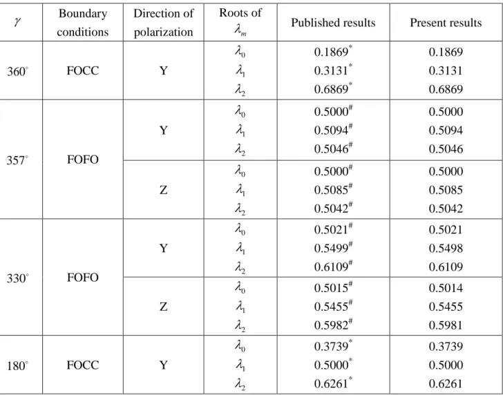
2.3. Verification of Solution

To validate the proposed solution, convergence studies for minimum Re[λ ] (real part _m

of λ ) are conducted by increasing the number of sub-domains or increasing the number of _m polynomial terms in each sub-domain, and the convergent solutions are compared with the published results. The wedges under consideration are made of piezoelectric material PZT-4, which is transversely isotropic. Table 2.1 presents the material properties of PZT-4.

Table 2.2 considers three cases. Four letters specify the boundary conditions of a wedge at 0

θ = and θ γ= . The first and third letters represent the mechanical boundary conditions at 0

θ = and θ γ= , respectively; and C and F represent clamped and free boundary conditions, respectively. Similarly, the second and fourth letters concern the electric boundary conditions with C and O’s denoting electrically closed and open boundary conditions, respectively. These rules are adopted throughout the paper.

The first case concerns a crack problem with a material having its direction of polarization in the z direction (see Fig. 1). The surfaces of the crack are free of surface traction and surface charge. That is σ =_θθ σ =_θ_r σ = D_θ_z _θ=0 at θ =0 and 2π . The results of Sosa and Pak (1990) were obtained by using an eigenfunction approach, which is similar to the present approach. Sosa and Pak (1990) examined a piezoelectric parallelepiped with a cut-through crack and having its direction of polarization in the z direction, so that they could find a closed-form solution forλ . _m

The other two cases involve 180o and 360o wedges with FOCC boundary conditions and polarization along θ =180o and θ =270o, respectively, in the plane x-y. Table 2.2 also

壓電材料迴轉體與楔形板幾何引致電彈奇異性之探討

行政院國家科學委員會補助專題研究計畫